| Issue |
A&A
Volume 630, October 2019
|
|
|---|---|---|
| Article Number | A81 | |
| Number of page(s) | 11 | |
| Section | Planets and planetary systems | |
| DOI | https://doi.org/10.1051/0004-6361/201935598 | |
| Published online | 24 September 2019 | |
A possibly inflated planet around the bright young star DS Tucanae A★,★★
1
INAF – Osservatorio Astronomico di Padova,
Vicolo dell’Osservatorio 5,
35122
Padova,
Italy
2
INAF – Osservatorio Astronomico di Palermo,
Piazza del Parlamento, 1,
90134
Palermo,
Italy
e-mail: This email address is being protected from spambots. You need JavaScript enabled to view it.
3
Dipartimento di Fisica e Astronomia – Universtà di Padova,
Vicolo dell’Osservatorio 3,
35122
Padova,
Italy
4
INAF – Osservatorio Astrofisico di Catania,
Via S. Sofia 78,
95123
Catania,
Italy
5
INAF – Osservatorio Astrofisico di Torino,
Via Osservatorio 20,
10025
Pino Torinese (TO),
Italy
6
Monash Centre for Astrophysics, School of Physics and Astronomy, Monash University,
Clayton
3800,
Melbourne,
Australia
7
Thüringer Landessternwarte Tautenburg,
Sternwarte 5,
07778
Tautenburg,
Germany
8
INAF – Osservatorio Astronomico di Trieste,
via Tiepolo 11,
34143
Trieste,
Italy
9
INAF – Osservatorio Astronomico di Capodimonte,
Salita Moiariello 16,
80131
Napoli,
Italy
10
Observatoire de Genève, Université de Genève,
51 ch. des Maillettes,
1290 Sauverny,
Switzerland
Received:
2
April
2019
Accepted:
19
July
2019
Abstract
Context. The origin of the observed diversity of planetary system architectures is one of the main topics of exoplanetary research. The detection of a statistically significant sample of planets around young stars allows us to study the early stages of planet formation and evolution, but only a handful are known so far. In this regard a considerable contribution is expected from the NASA TESS satellite, which is now performing a survey of ~85% of the sky to search for short-period transiting planets.
Aims. In its first month of operation TESS found a planet candidate with an orbital period of 8.14 days around a member of the Tuc-Hor young association (~40 Myr), the G6V main component of the binary system DS Tuc. If confirmed, it would be the first transiting planet around a young star suitable for radial velocity and/or atmospheric characterisation. Our aim is to validate the planetary nature of this companion and to measure its orbital and physical parameters.
Methods. We obtained accurate planet parameters by coupling an independent reprocessing of the TESS light curve with improved stellar parameters and the dilution caused by the binary companion; we analysed high-precision archival radial velocities to impose an upper limit of about 0.1 MJup on the planet mass; we finally ruled out the presence of external companions beyond 40 au with adaptive optics images.
Results. We confirm the presence of a young giant (R = 0.50 RJup) planet having a non-negligible possibility to be inflated (theoretical mass ≲ 20 M⊕) around DS Tuc A. We discuss the feasibility of mass determination, Rossiter-McLaughlin analysis, and atmosphere characterisation allowed by the brightness of the star.
Key words: planets and satellites: fundamental parameters / techniques: photometric / techniques: spectroscopic / techniques: radial velocities / techniques: imaging spectroscopy / stars: individual: DS Tuc A
Based on observations made with ESO Telescopes at the La Silla Paranal Observatory under programme IDs 075.C-0202(A), 0102.C-0618(A), 0103.C-0759(A), 075.A-9010(A), 076.A-9006(A), 073.C-0834(A), 083.C-0150(B).
This paper includes data collected by the TESS mission, which are publicly available from the Mikulski Archive for Space Telescopes (MAST).
© ESO 2019
1 Introduction
A few decades after the first detection, exoplanetary science is shifting from the discovery of exoplanets to understanding the origin of their astonishing diversity. The frequency of planets as a function of their mass, size, and host star properties is a key parameter for testing the diverse outcomes of planet formation and evolution. They are the result of the complex interplay between a variety of physical and dynamical processes operating on different timescales during their formation and successive orbital evolution. These processes are in turn dependent on environmental conditions, such as disc properties, multiplicity, and stellar radiation fields, and involve mainly migration processes. For instance, a smooth planet migration through the protoplanetary disc (Baruteau et al. 2014) can be revealed by low orbital eccentricities and spin–orbit alignments and operates on very short timescales (less than 10 Myr, i.e. the disc lifetime), while the long-term high-eccentricity migration (acting typically up to 1 Gyr; Chatterjee et al. 2008) can result either in circular, aligned orbits and short periods or eccentric, misaligned orbits and long periods. Moreover, according to the Coplanar High-Eccentricity Migration (CHEM, Petrovich 2015), the existence of hot and warm Jupiters could be due to secular gravitational interactions with an eccentric outer planet in a nearly coplanar orbit, implying that a short-period gaseous planet could be coupled to other distant bodies (of planetary or stellar nature).
In this context the detection of young planets at short or intermediate orbital periods is crucial to investigate the regimes of planet migration. However, the high level of stellar activity in young stars heavily prevents the detection of planetary signals with the radial velocity (RV) method, and the estimates on the frequency provided to date (Donati et al. 2016; Yu et al. 2017) still rely on small numbers and suffer from claimed detections that have not been confirmed by independent investigations (e.g. Carleo et al. 2018).
The NASA Transiting Exoplanet Survey Satellite (TESS; Ricker et al. 2015) is expected to play a crucial role in this framework. Being a space-borne full-sky survey, for the first time it will produce precise light curves for thousands of young stars, in turn providing planetary candidates that will require external validation, however.
In this paper we validate the first young planet candidate spotted by TESS around one of the two components of the DS Tuc binary, the G6V star DS Tuc A (HD 222259, V = 8.47), member of the Tuc-Hor association. This target (TESS Input Catalog ID: TIC 410 214 986) was observed in the first sector of TESS (25 Jul–22 Aug, 2018), in both short (2 min) and long (30 min) cadence and, because transit signatures have been found, has been tagged as TOI-200 (TESS Object of Interest; see the TOI releases webpage1).
In the following we confirm the planetary nature of the potential candidate around DS Tuc A by using data available in the public archives. First, we revise the stellar parameters of the host (Sect. 2). Then we propose our analysis of the TESS light curve, including a transit fit that considers the impact of the stellar companion on the estimation of the planet parameters (Sect. 3). We present our evaluation on RVs and adaptive optics data used to constrain the planetary mass and the presence of additional bodies in the system (Sect. 4). Finally, we present our discussion and conclusions in Sect. 5.
2 Stellar parameters
DS Tuc is a physical binary formed by a G6 and a K3 component at a projected separation of 5.4 arcsec (240 au at a distance of 44 pc). The stellar parameters, some of which are updated in our study, are listed in Table 1.
The system is included among the core members of the Tuc-Hor association (e.g. Zuckerman & Webb 2000). High levels of magnetic activity, a strong 6708 Å lithium line, and its position on the colour–magnitude diagram slightly above the main sequence strongly support a young age. The kinematic analysis, based on Gaia DR2 results and the online BANYAN Σ tool (Gagné et al. 2018), yields a 99.9% probability of membership in the Tuc-Hor association. Its age is estimated to be 45 ± 4 Myr from isochrone fitting (Bell et al. 2015), ~40 Myr from lithium depletion boundary (Kraus et al. 2014), and  from kinematics (Crundall et al. 2019). We adopt in the following the 40 Myr as the mean value of these three determinations based on independent methods.
2.1 Spectroscopic analysis
In order to get a metallicity estimate of the system, we carried out spectroscopic analysis of DS Tuc A, by exploiting a high-resolution, high signal-to-noise spectrum acquired with FEROS (nominal resolution R = 48 000; Kaufer et al. 1999). The spectrum was reduced with the modified version of the ESO pipeline described inDesidera et al. (2015). Performing abundance analyses for very young stars (age ≲ 50 Myr) is not straightforward and presents several issues that hinders a standard approach. For instance, microturbulent velocity (vt) values for stars of this kind are found to be extremely large, reaching 2.5 km s−1. This might be due to the presence of hot chromospheres, which affect the strong Fe I lines forming in the upper atmosphere layers (we note the trend of Fe abundances with line formation depth found by e.g. Reddy & Lambert 2017). An extensive discussion of this topic will be presented in a dedicated series of papers, focussing on the abundance determination of pre-main sequence stars (D’Orazi et al., in prep.; Baratella et al., in prep.). Here we briefly describe our new approach: effective temperature (Teff) is fixed from photometry, whereas we use Ti lines to optimise microturbulence and gravity by imposing the ionisation equilibrium condition such that logn(Ti I) and logn(Ti II) abundances agree within the observational uncertainties. The exploitation of Ti lines presents two main advantages: (i) the oscillator strengths of the lines (log gf) have been experimentally determined by Lawler et al. (2013), and (ii) the titanium lines form at an average formation depth of ⟨ log τ5⟩~−1 (Gurtovenko & Sheminova 2015), thus quite deep in the stellar photosphere. As a consequence, they are not strongly affected by chromospheric activity.
Our results provide Teff = 5542 ± 70 K, log g = 4.60 ± 0.1 dex, vt = 1.18 ± 0.10 km s−1, logn(Ti I) = 5.02 ± 0.08 (rms), and logn(T II) = 84.94 ± 0.07. We inferred a metallicityof [Fe/H] = − 0.08 ± 0.02 ± 0.06, where the first uncertainty is the error on the mean from the Fe I lines, and 0.06 dex uncertainty is related to the atmospheric stellar parameters. The slightly subsolar metallicity is consistent with a previous determination for the Tuc-Hor association by Viana Almeida et al. (2009). We refer the reader to our previous works for details on error computation (e.g. D’Orazi et al. 2017). Unfortunately, we could not perform a spectroscopic parameter determination for the DS Tuc B component. Because at the relatively low temperature (Teff ~ 4600 K), over-ionisation effects for iron and titanium lines are at work in stars younger than roughly 100 Myr. The difference between logn(Fe I) and logn(Fe II) and/or logn(Ti I) and logn(Ti II) are larger than 0.8 dex, resulting in unreliable (unphysical) parameters and abundances. This kind of over-ionisation and over-excitation effects have been noticed in several young clusters, such as NGC 2264 (King et al. 2000), the Pleaides (King et al. 2000; Schuler et al. 2010), M34 (Schuler et al. 2003), and IC 2602 and IC 2391 (D’Orazi & Randich 2009).
Stellar properties of the components of DS Tuc.
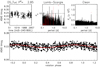 |
Fig. 1 Time series, periodogram, and phase curve of the ASAS photo- metric data of DS Tuc, collected between 2000 and 2008. |
2.2 Rotation period
DS Tuc was observed as part of the All Sky Automated Survey (ASAS; Pojmanski 1997) from 2000 to 2008. From the public archive we retrieved a total of 560 V -band measurements with an average photometric accuracy of σ = 0.031 mag. The time series is shown in the upper left panel in Fig. 1, where a long-term photometric variation, probably due to a spot cycle, is clearly seen. The complete time series was analysed with the Lomb-Scargle (Scargle 1982) and CLEAN (Roberts et al. 1987) periodograms (Fig. 1, upper central and right panels). Both methods returned a rotation period P = 2.85 ± 0.02 days with a false alarm probability (FAP) < 0.01. The FAP was computed with Monte Carlo simulations (e.g. Messina et al. 2010), whereas the uncertainty on the rotation period was derived following Lamm et al. (2004). Periodograms were also computed for segments of the whole time series and the same rotation period was retrieved in 5 out of 12 segments.
We obtained an independent measure of the Prot value from the TESS short-cadence light curve extracted after masking the transit events (see details in Sect. 3.1). The autocorrelation function analysis (e.g. McQuillan et al. 2013) shows the first peak at 2.91 days, while the generalised Lomb-Scargle (GLS) periodogram (Zechmeister & Kürster 2009) recovered the expected signal at 2.85 days with an amplitude of 16 millimag in the TESS passband after removing the contribution of the binary companion. Finally, we measured the rotational period with its error by modelling the light curve using a Gaussian process (GP) with a quasi-periodic kernel. We made use of the PyORBIT code (Malavolta et al. 2016, 2018), following the prescriptions in Rice et al. (2019), with the GP computed by the george package (Ambikasaran et al. 2015). Following López-Morales et al. (2016), we imposed a prior on the coherence scale to allow a maximum of three peaks per rotational period2. To speed up the computation, we binned the light curve in steps of 1 h. We measured a rotation period of Prot = 2.99 ± 0.03 days, with a covariance amplitude of λTESS = 11 ± 2 millimag and an active region decay timescale of Pdec = 3.12 ± 0.20 days. The GP and the autocorrelation function are more sensitive to the evolution of the active regions, which explains the slight discrepancy (of the order of 5%) of the estimated Prot with respect to the GLS and LS periodograms methods.
In the following we adopt as a rotation period of the target the value obtained from ASAS data.
2.3 Parameters
The radii and masses of the components were derived using the PARAM interface (da Silva et al. 2006). By fixing conservative age boundaries between 30 and 60 Myr from the Tuc-Hor membership, adopting the effective temperature (with an error of 70 K) from Pecaut & Mamajek (2013), and the spectroscopic value of metallicity, we obtain mass and radius values of 0.96 M⊙ and 0.87 R⊙ for DS Tuc A, and 0.78 M⊙ and 0.77 R⊙ for the B component. Our stellar radius is very similar to that derived in Gaia DR2.
The stellar radius of the primary, coupled with the observed rotation period yields a rotational velocity of 15.5 km s−1, in agreement with our determination of 15.5 ± 1.5 km s−1 (from spectral synthesis, as in e.g. D’Orazi et al. 2017). This suggests that the star is seen close to equator-on. The observed motion of the binary components on the plane of the sky is nearly radial, suggesting a very eccentric and/or a very inclined orbit (close to edge-on).
Finally, the star has no significant IR excess (Zuckerman et al. 2011), which excludes prominent dust belts around it.
3 TESS light curve analysis
In this section we present our extraction and analysis of the TESS light curve of DS Tuc.
3.1 Light curve extraction
DS Tuc was observed in the first sector of TESS for 27 days, falling on the CCD 2 of Camera 3. We extracted the light curve from the 30-min cadence full frame images (FFIs) exploiting the TESS version of the software img2lc developed by Nardiello et al. (2015) for ground-based observations, and also used for Kepler images by Libralato et al. (2016). Briefly, using the FFIs, empirical point spread functions (PSFs) and a suitable input catalog (in this case Gaia DR2, Gaia Collaboration 2018), the routine performs aperture and PSF-fitting photometry of each target star in the input catalog, after subtracting the neighbours located between 1 px and 25 px from the target star. A detailed description of the pipeline will be given by Nardiello et al. (in prep.). For the 2-min. cadence, we adopted the raw light curve (PDCSAP_FLUX) released by the TESS team and available for download from the Mikulski Archive for Space Telescopes (MAST) archive.
We corrected both the 2- and 30-min cadence light curves of DS Tuc adopting the same procedure described in Nardiello et al. (2016). For each star with GBP < 13 located on the CCD 2 of Camera 3, we computed the mean and the rms of its light curve. We selected the 25% of the stars with the lowest rms, and we used them to extract a cotrending basis vector (CBV) adopting the principal component analysis. We applied the Levenberg–Marquardt method to find the coefficient A that minimises the expression 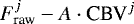 , where
  is the raw flux of the star at time j, with j = 1,..., Nepochs, and Nepochs the number of points in the light curve. We cotrended the light curve subtracting A ⋅ CBV to the light curve of DS Tuc. In Fig. 2 we show the 2-min (blue points) and the 30-min (red points) cadence before (top) and after (bottom) the correction. Three transit events can be found in the time series (dashed lines in Fig. 2), but the third event occurred during a temporary failure of the satellite pointing system (1347 ≤TJD ≤ 1349, where TJD = JD−2 457 000), with a consequent degradation of the data (upper panel of Fig. 2). Thanks to our alternative detrending algorithm we were able to recover the third transit, although at a lower quality with respect to the others.
The TESS light curve of DS Tuc shows evidence for transits of two distinct companions. According to the Data Validation Report associated with each candidate (see Twicken et al. 2018), one of the signals could be related to a companion with an orbital period of 20.88 days; however, after a first inspection of the light curve, the results of the fitting procedure, and matching the stellar field with Gaia DR2 data (see also Sect. 4.2), it shows a very high probability of being a false positive, possibly due to an instrumental effect. The second signal appears to be produced by a real companion, characterised by an orbital period of 8.138 days (semi-major axis = 0.09 au) and a planet radius of 8.3 R⊕, evaluated adopting the stellar radius from the TESS Input Catalog (1.19 ± 0.13 R⊙, Stassun et al. 2018) which is significantly larger with respect to the one we obtained (see Sect. 2.3) and also reported by Gaia. Moreover, since the projected separation of the two stellar companions of the binary system is 5.36″, and the TESS pixel scale is 21″ pix−1, the two sources are not resolved, leading to a likely overestimation of the planetary radius as a consequence of the dilution of the transit by the binary companion. Before proceeding, we verified via a centroid analysis from the TESS full-frame images that the transit of the eight-day period candidate occurred on the primary star. Figure 3 shows the considered field, limited by the 3-pixel aperture used for the flux extraction (red circle), with grey dots indicating the positions of DS Tuc A and B and a faint background source. The plot shows the calculated offsets (and the corresponding error bars) with respect to the TESS out-of-transit images (magenta) and to the position reported in Gaia DR2 (blue). In both cases, the offset falls within one sigma of the position of DS Tuc A.
In the next two sections, we present our model of the extracted light curve developed via two different approaches: the first considers only the first two transits and simultaneously fits the rotational modulation, the second considers all the available transits and a different method of flattening the curve. The two methods lead to consistent results, but we decided to adopt the planet parameters from the first one.
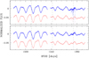 |
Fig. 2 Light curve of DS Tuc before (top) and after (bottom) the correction of the systematic effects. Each panel shows the 2-min. (Red points) and 30-min. (Blue points) cadence light curve. BTJD is the Barycentric TESS Julian Day, corresponding to BJD −2 457 000. The dashed lines represent the location of the three detected transits of DS Tuc A b. |
3.2 Two-transit fit
In the first approach, a temporal window of 0.6 days (roughly five times the duration of the transit) was selected around each mid-transit time, which allowed us to approximate the rotational modulation with a second-order polynomial for each transit. The analysis wasperformed with PyORBIT, a convenient wrapper for the transit modelling code batman (Kreidberg 2015) and the affine invariant Markov chain Monte Carlo sampler emcee (Foreman-Mackey et al. 2013) in combination with the global optimisation code PyDE3. Our model included the following as parameters: the time of first transit Tc, the planetary period P, the impact parameter b, the planetary to stellar radius Rp ∕R⋆, and the stellar density in units of solar density ρ⋆. The dilutionfactor FB∕FA was included as a free parameter to account for its impact on the error estimate of Rp, with a Gaussian prior derived from the Gaia and J magnitudes of the A and B components of the stellar system transformed into the TESS system by using the relation in Stassun et al. (2018)4. For each transit we also included a jitter term, quadratically added to the photon noise estimate of the TESS light curve, to take into account short-term stellar activity noise and unaccounted TESS systematics. We tested eight different models to fit the TESS light curves: without priors on the limb darkening (LD) coefficients u1 and u2, prior only on u1, prior only on u2, and priors on both coefficient. Each model was repeated, twice for the circular orbit and twice for Keplerian orbit. The priors on the LD coefficients were computed through a bilinear interpolation of the grid presented by Claret (2018), considering Teff, log g, and metallicity in Table 1. We followed the prescriptions of Kipping (2013) for the parametrisation of the LD coefficients, and the ( ,
,  ) parametrisation for eccentricity and argument of pericentre (Eastman et al. 2013). We accounted for the 120 s exposure time of TESS when modelling the transit (Kipping 2010). All the parameters were explored in linear space, with the exception of the photometric jitter terms. Our models have 16 free parameters for the circular orbit cases, and 18 for the Keplerian cases. We deployed a number of walkers equal to eight times the dimensionality of the problems, for a total of 128 and 144 walkers. For each model we ran the sampler for 50 000 steps, we then applied a burn-in cut of 15 000 steps and a thinning factor of 100, obtaining a total of 44 800 and 50 400 independent samples for the circular and Keplerian models, respectively. Confidence intervals of the posteriors were computed by taking the 34.135th percentile from the median (Fig. 4). The fit was performed after rescaling the flux for its median value. In addition to the MCMC fit, we performed the model selection by computing the Bayesian evidence with the nested sampling algorithm PolyChord (Handley et al. 2015). Models with a prior on one or both the LD coefficients are disfavoured, although not significantly, with respect to the model without priors. We found that all the parameters are consistent across the models, with the exception of the LD coefficients that show a mismatch with the selected priors, favouring the choice of uninformative priors to exclude unphysical solutions (in agreement with Kipping 2013). The discrepancy between the literature and derived values for the limb darkening coefficients is likely the consequence of the strong magnetic field of the star, as investigated by Beeck et al. (2015) and confirmed in Maxted (2018).
To improve the precision of both the mid-transit ephemeris and the orbital period, we repeated the same modelling by including the recovered third transit in the fit (and a third second-order polynomial for the detrending). The results are fully consistent with the previous model and returned the same uncertainties. Since the inclusion of the third transit does not improve the parameter determination, and the light curve is probably affected by instrumental systematics, we considered this model only for the estimation of T0 and for the orbital period. We list in Table 2 the values obtained when assuming a circular orbit for the planet and no priors on the LD coefficients, while the resulting model is superimposed on the TESS light curves in Fig. 5 (black line). The value of the first coefficient of the two second-order polynomials used to correct the raw transit light curves reflects the inclusion of the dilution factor. The amount of jitter of the first transit is higher than the second, suggesting that the variation in the amplitude of the light curve within the time span of the TESS observation could be due to a variation in the stellar activity (cf. Fig. 2). The resulting planetary radius is 5.6 ± 0.2 R⊕, after takinginto account the uncertainty on the stellar radius. This value decreases by ~ 20% when we neglect the dilution effect. As in the case of the LD coefficients mentioned above, magnetic activity can also affect the evaluation of other parameters of the star. For instance, the stellar radius can be inflated by up to 10%, as pointed out by Chabrier et al. (2007) and López-Morales (2007), with a possible impact on the planetary radius estimation. In the worst case, we could expect an increase in the planet radius of about 15–20%.
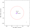 |
Fig. 3 Difference image centroid offset for DS Tuc A from TESS observations. The grey dots indicate the position of the sources in the field, the red circle indicates the extension of the photometric aperture, while the magenta and blue crosses with error bars represent the offset with respect to the TESS out-of-transit images and the coordinates of the target from Gaia DR2. |
3.3 Alternative modelling of three-transit signals
In our alternative approach for transit modelling, we flattened the extracted light curve with different approaches and window size: running median, running polynomial of different order, and a cubic spline on knots. We applied the flattener algorithm after splitting the light curve at the TESS downlink time. We determined that the best flattened light curve, having the smallest 68.27th percentile scatter around the median value, is a running polynomial of third order with a window size of 0.55 days with respect to the median of the normalised flux. This scatter metric was used to remove outliers with an asymmetric sigma clipping: 5σ above and 10σ below the median of the flux. In addition, the deviation measures the photometric scatter of the light curve and we used it as the error on the light curve. We searched for the transit signal on the flattened light curve with TransitLeastSquares (TLS, Hippke & Heller 2019). We found a transit-like signal with a period of 8.13788 ± 0.03704 d, a depth of 1830 ppm, a total duration (T14) of about 172 min, and a signal detection efficiency (SDE, Alcock et al. 2000) of 17.58, which is higher than the thresholds reported in Hippke & Heller (2019). The TLS found three transits in the light curve, and we selected a portion of ± 2 × T14 around each transit time (T0) of the extracted light curve (not flattened). We simultaneously modelled the three transits with the batman-package (Kreidberg 2015) and analysed the posterior distribution with emcee (Foreman-Mackey et al. 2013). We fit as common parameters across the three transits a dilution factor parameter (ratio of the flux of the secondary star to the primary, FB ∕FA), the stellar density in gr cm−3, the logarithm in base two of the period of the planet (log2P), the ratio of the radii (k = Rp∕R⋆), the impact parameter (b), the parameters q1 and q2 introduced in Kipping (2013) for a quadratic limb darkening law, the logarithm in base two of a jitter parameter (log2σj), and the reference transit time (T0,ref). For each transit light curve, we fitted three coefficients for a quadratic detrending (c0, c1, c2), and a transit time (T0). All the fitted and physical parameters were bounded to reasonable values. In particular the period was bounded within 8.13788 ± 10 × 0.03704 d, all the T0 were limited within the TLS estimate ± T14 BTJD, and we used the central transit times to bound the T0,ref ± T14. We assumed a circular orbit for the planet. We used the stellar parameters from Sect. 2 to determine an asymmetric Gaussian prior on the stellar density (![Mathematical equation: $\mathcal{N}(2.00,[-0.21,+0.24])$](/articles/aa/full_html/2019/10/aa35598-19/aa35598-19-eq6.png) ). The prior on the dilution factor was computed as in Sect. 3.2. We ran emcee with 60 chains (or walkers) for 50 000 steps, and then we discarded the first 20 000 steps as burn-in after checking the convergence of the chains (visual inspection and Gelman-Rubin
). The prior on the dilution factor was computed as in Sect. 3.2. We ran emcee with 60 chains (or walkers) for 50 000 steps, and then we discarded the first 20 000 steps as burn-in after checking the convergence of the chains (visual inspection and Gelman-Rubin  ). We obtained the parameter posteriors after applying a pessimistic thinning factor of 100. We computed the confidence intervals (CI) at the 16th and 84th percentiles and the high-density intervals (HDIs, corresponding to the 16th and 84th CI percentiles). The parameters, determined as the maximum log-likelihood estimator (MLE) within the HDI and the median of the posterior distributions, are given in Table A.1 and are consistent within 1σ with the analysis presented in Sect. 3.2. Even in this case, a model with no priors on LD coefficients is preferred, according to the Bayesian information criterion (BIC). The three transits with the median best-fit model are shown in Fig. 6.
4 Planet validation
4.1 Radial velocity and other spectroscopic time series
Five spectraof DS Tuc A, spanning 100 days, were obtained in 2005 with HARPS (at the 3.6 m telescope at ESO – La Silla) and the data, reduced with the standard pipeline, are available from the ESO Archive. Three additional spectra have recently been collected (Nov. 2018 and June 2019) and are included in our dataset. However, the HARPSstandard reduction, performing the cross-correlation function (CCF) of the spectrum with a digital maskrepresenting the typical spectral features of a G2 star (Pepe et al. 2002) is not suitable for a fast rotator like DS Tuc A, so we reprocessed the spectra with the offline version of the HARPS data reduction software (DRS, C. Lovis, priv. comm.), where the width of the computation window of the CCF can be adapted according to the rotational broadening. In this case, we used 240 km s−1. The resulting RVs are listed in Table 3. We also employed the TERRA (Anglada-Escudé & Butler 2012) and SERVAL (Zechmeister et al. 2018) pipelines to obtain alternative RV measurements for comparison.
When joining the two datasets, separated by 13 yr, we must take into account an RV offset produced by a change in the HARPS set-up that occurred in 2015, which is on average ~ 16 m s−1 for G-type slowly rotating stars, as reported by Lo Curto et al. (2015). In particular, these authors found a dependence of the RV shift on the width of the spectral lines, which in the case of DS Tuc A are particularly broadened. However, a comparison between old and new RV measurements for different types of stars, including young objects and fast rotators, shows that the average offset is compatible within the errors with respect to the result in Lo Curto et al. (2015). In our case, we found an offset between the two series of about 32 ± 77 m s−1, significantly lower than the scatter of the data.
The RV dispersion of the time series is ~ 174 m s−1 for HARPS offline DRS, ~ 136 m s−1 for TERRA,and 172 m s−1 for SERVAL, with corresponding median RV error of 7.6, 6.2, and 3.1 m s−1. The lower dispersion for TERRA is due to the algorithm used, which better models the distorted line profile of both M dwarfs and active stars, and is thus particularly suitable to obtain RVs for objects of this kind, as already shown by Perger et al. 2017. Finally, we measured several activity indicators: the bisector span (see Table 3) and the  , directly provided by the HARPS DRS; Hα (as in Gomes da Silva et al. 2011); the chromatic index (as derived by SERVAL); and ΔV, Vasy,mod, and an alternative evaluation of the bisector through the procedure presented in Lanza et al. (2018). All of these indicators show a clear anti-correlation with respect to the RVs obtained with all the pipelines, as expected for a young and active star for which the rotation dominates the RV signal (see the upper panel of Fig. 7). An outlier is present in the time series, not related to the processing method since all the pipelines report the same anomalous value. On the other hand, there is no indication of flare or signal of peculiar activity in that spectrum, or problems in data collection (such as lowsignal-to-noise ratio (S/N), high airmass or lunar contamination). For this reason, we included this datum in our analysis. The Spearman correlation coefficient, between the RVs and the bisector is approximately − 0.97 for the three datasets, with a significance of ~2 × 10⁻⁴, evaluated through the IDL routine SAFE_CORRELATE. When we subtract this correlation from the RVs (e.g. HARPS DRS dataset), the dispersion of the residuals decreases from ~ 200 to ~ 100 m s−1, from which we obtain a first approximation of the upper limit on the planet real mass (since we know the inclination of the orbit i = 88.8°), which would be around 1.3 MJup. It is reasonable to expect that these residuals are still affected by an additional contribution of the stellar activity, and a significantly lower value of the planetary mass is more likely. According to the empirical mass–radius relations provided by Bashi et al. (2017), we should expect a planetary mass of 22.9 ± 2.5 M⊕. However, we must take into account that the relations are deduced from a sample of well-characterised exoplanets, generally hosted by mature stars, that may not be applicable to young objects still experiencing their contraction phase. By using the orbital elements from Table 2 and considering an RV semi-amplitude compatible with the estimated mass upper limit from our data and the mass from the empirical relation, we obtain RV models to compare with the residuals. The lower panels of Fig. 7 show that the RV residuals are compatible with those planetary masses (green and blue line, respectively). However, we note that a full analysis of the activity is not fully reliable with the available data, due to their sparse sampling.
As a further check, by using the same RV residuals we evaluated the corresponding period-mass detection limits, based on the comparison of the variance of the RV time series with and without a variety of planet masses and periods added to the data, using the F test as in Desidera et al. (2003). Figure 8 shows that we can rule out the existence of planetary companions with m sini higher than 2–3 MJup with an orbital period shorter than 10 days, while the detection threshold is less sensitive (M ~ 7 MJup) at about 100 days.
The observed RV dispersion of DS Tuc A is within the range of dispersion for stars with similar age and spectral type, derived from HARPS spectra of several objects available in the ESO archive, further supporting the magnetic activity as the dominant source of variability (e.g. Kraus et al. 2014). The CCF and line profile indicators also show the typical alterations due to the presence of active regions, without any indication of a double-lined spectroscopic binary.
High-resolution HARPS spectra are available only for the primary star. However, RV monitoring the secondary is available from Torres et al. (2006), resulting in a low dispersion of 0.1 km s−1 (for six spectra obtained with FEROS), ruling out the presence of close stellar companions for the secondary as well. More in general, the similar absolute RVs reported by several authors for the two components (see Table 1) argue against any RV variation exceeding 1 km s−1 over a baseline of decades.
Parameters for DS Tuc A b.
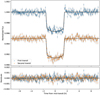 |
Fig. 5 Upper panel: TESS light curves of the two transits of DS Tuc A b and the adopted fit (black line). Lower panel: residuals of the light curves after the subtraction of the model. |
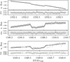 |
Fig. 6 TESS undetrended light curves of the three transit events of DS Tuc A b, with the corresponding fit. |
Radial velocities from DS Tuc A HARPS spectra with uncertainties as obtained from the HARPS offline DRS and the corresponding measure of the bisector span with uncertainties derived via the procedure described in Lanza et al. (2018).
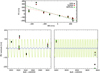 |
Fig. 7 Upper panel: correlation between HARPS bisector span and RVs obtained from the three different pipelines. Lower panels: timeseries of the RV residuals after removing the correlation from HARPS RVs (same colour-coding as for the pipelines). The solid lines represent the RV signal in the case of a planet with the same orbital elements as DS Tuc A b and a semi-amplitude corresponding to the mass upper limit estimated from the residuals (green line) and from empirical relation (blue line). |
 |
Fig. 8 Detection limits of the RV time series of DS Tuc A with a confidence level of 95%. |
4.2 Constraints from direct imaging
We exploited the datasets in the L′ spectral band from the Nasmyth Adaptive Optics System Near-Infrared Imager and Spectrograph (NaCo), mounted at the Very Large Telescope, ESO – Paranal Observatory, Chile, taken on 3 Sept. 2004 and published in Kasper et al. (2007) and in Ks band taken on 30 Sept. 2009 and published in Vogt et al. (2015). Both datasets were reduced following the methods devised in the original papers and were then registered in such a way that the primary star was at the centre of the image. To improve the contrast in the regions around the two stars we subtracted the PSF of the other component following the method presented in Desidera et al. (2011) and in Carolo et al. (2014). The contrast limit was then calculated using the same method described in Mesa et al. (2015). We display the contrast plots for both epochs and for both stars in Fig. 9.
We used these contrast values to define mass detection limits around both stars of the binary, assuming the age and distance values given in Table 1 and exploiting the AMES-COND evolutionary models (Allard et al. 2003). The final results of this procedure are displayed in Fig. 10 for both the observing epochs and for both the stars of the binary. For the primary star, we were able to exclude the presence of objects with mass larger than ~7–8 MJup at separations larger than 40 au. The mass limits around the secondary are slightly higher.
The ~5 yr time baseline between the two NaCo observations coupled with the proper motion and parallax of the star implies a relative shift of 524 mas for a stationary background object with respect to DS Tuc. Therefore, from the detection limits in Fig. 9, a stationary background source responsible for the transit feature (Δ mag smaller than about 5.5 mag assuming 0.75 mag eclipse depth) would have been detected in at least one of the two epochs and is then ruled out by the observations. The only remaining false alarm sources are represented by bright stellar companions at projected separations smaller than ~10 au, but large physical separations, considering the detection limits from RVs and imaging. This configuration is extremely unlikely from the geometrical point of view and is made negligible by the presence of DS Tuc B at 240 au. The imaging observation reported here and the analysis of sources within TESS PSF from Gaia DR2 do not allow us to reliably identify candidates that are responsible for the false alarm reported in the original TESS alert. Most likely the corresponding photometric signal is not of astrophysical origin.
Coupling the results of the RV monitoring and the NaCo observations, the presence of an additional companion responsible for the photometric dimming observed with TESS is extremely unlikely. Gaia DR2 results indicate that there are no additional sources brighter than G = 18.3 (10 mag fainter than the primary) within 1 arcmin.
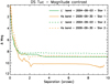 |
Fig. 9 Contrast plot in Δ Mag obtained around both stars of the binary for the 2004 and the 2009 observation. |
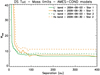 |
Fig. 10 Mass detection limits expressed in MJup as a function of the separation from the stars expressed in au for both observing epochs and for both the stars of the binary. |
4.3 Falsepositive probability
As a final step, we ran the free and open source validation tool vespa (Morton 2012, 2015) to evaluate the false positive probability (FPP) of DS Tuc A b in a Bayesian framework. The vespa tool has been widely used (e.g. Montet et al. 2015; Crossfield et al. 2016; Malavolta et al. 2018; Mayo et al. 2018; Wells et al. 2019) to estimate the probability that a given signal is actually produced bya real planet and is not the result of different astrophysical configurations. As reported in Morton (2012), the false positive scenarios explored by vespa are (i) a non-associated background or foreground eclipsing binary blended inside the photometric aperture of the target (BEB), (ii) a hierarchical triple system where two components eclipse (HEB), (iii) an eclipsing binary (EB), and (iv) a non-associated blended background or foreground star hosting a transiting planet (Bpl). For each configuration, the code simulates a representative stellar population, which in our case is constrained by the information provided in Tables 1 and 2 (coordinates, optical and near-infrared photometry, orbital period, and the ratio of planet to star radius) and the observed TESS light curve and NaCo contrast curve. Different false positive scenarios are considered for those populations, and are used to define the prior likelihood that a specific configuration actually exists (i.e. that is consistent with the input data) and the likelihood of transit for those configurations. The comparison with the full set of scenarios allows us to evaluate the FPP: if the FPP is significantly lower than 0.01, the planet is validated. We ran vespa with the available data of DS Tuc A b and obtained an FPP lower than 10−6, resulting in a full validation of the transiting planet scenario. Curiously, a large fraction of BEB configurations are in principle permitted by the data (upper left pie chart in Fig. 11), but the fitting of the input transit signal clearly favours the planet hypothesis (upper right pie chart in Fig. 11).
5 Discussion and conclusions
In this paper we have ruled out blending scenarios and then validated the planet candidate found with TESS around the primary component of the young binary system DS Tuc, confirmed member of the Tuc-Hor association. We estimated the transit parameters, in particular the planet radius, taking into account the dilution effect due to the stellar companion of the host star. The comparison with theoretical models, accounting for the young age of the hosts, by Baraffe et al. (2003) and Linder et al. (2019), provides a mass below 20 M⊕, compatible with the empirical estimation of ~22 M⊕, suggesting that DS Tuc A b could be a super-Earth or no more than a Neptune-like planet. However, we note that these models are not optimised for heavily irradiated planets around young stars (i.e. they do not consider the possible inflation of the planetary radii).
The relatively low mass expected for the planet makes the detection of the RV signature quite challenging considering the amplitude of the activity jitter, as shown in Sect. 4.1. According to our simulations, an intensive monitoring (e.g. ~ 60 RV epochs spanning three months), coupled with appropriate modelling of the activity would allow the recovery of a signal with RV semi-amplitude down to ~ 6.5 m s−1 (corresponding to 20 M⊕) with an accuracy of 1σ, and a detection significance of 2σ in the case of an activity signal of the order of 100 m s−1. More promising is the perspective for the detection of the Rossiter-McLaughlin effect (RM), as its amplitude depends on planetary radius and not on planetary mass, and increases with the projected rotational velocity of the star. Furthermore, the activity noise is expected to be much smaller on the timescales of a single transit with respect to the few weeks or months needed for the orbit monitoring. Assuming the values in Tables 1 and 2, the RM signature should be around ~ 60 m s−1 (Eq. (40) in Winn 2010). Considering the moderately long period of the planet and the young age of the system, the spin–orbit angle is expected to be close to the original value, with little alteration due to tidal effects. The measurement of the RM effect would then give important insights into the migration history of the planetary system. Furthermore, the binarity is an additional reason for the specific interest in the RM determination. Finally, due to the high value of the v sini, this target can be studied with the tomographic technique.
The expanded structure of the planet favours the detection of strong atmospheric features. The scale height, obtained according to the equilibrium temperature (~900 K) is 1200 km, so the expected signal of the transmission spectrum feature is about 2 × 10⁻⁴. According to our evaluations, DS Tuc A b is the first confirmed transiting planet around a star ~ 40 Myr in age that can be characterised in full.
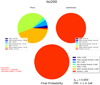 |
Fig. 11 Summary of the FPP evaluation obtained with vespa. Acronyms of the false positive scenarios are defined in Sect. 4.3. |
Acknowledgements
The authors thank the anonymous referee for the interesting comments and suggestions that improved the quality and robustness of the paper. We acknowledge the support by INAF/Frontiera through the “Progetti Premiali” funding scheme of the Italian Ministry of Education, University, and Research. The authors acknowledge Dr. A. Santerne, Dr. A. F. Lanza, and Dr. F. Borsa for their kind and useful suggestions. L.M. acknowledges support from PLATO ASI-INAF agreement n.2015-019-R.1-2018. L.Bo. acknowledges the funding support from Italian Space Agency (ASI) regulated by Accordo ASI-INAF n. 2013-016-R.0 del 9 luglio 2013 e integrazione del 9 luglio 2015. M.E. acknowledges the support of the DFG priority programme SPP 1992 “Exploring the Diversity of Extrasolar Planets” (HA 3279/12-1). We acknowledge the use of public TESS Alert data from pipelines at the TESS Science Office and at the TESS Science Processing Operations Center. Funding for the TESS mission is provided by NASA’s Science Mission directorate. During the final stages of preparation of this paper, we learned of an independent analysis prepared by another team (Newton et al. 2019).
Appendix A Additional table
References
- Alcock, C., Allsman, R., Alves, D. R., et al. 2000, ApJ, 542, 257 [NASA ADS] [CrossRef] [Google Scholar]
- Allard, F., Guillot, T., Ludwig, H.-G., et al. 2003, IAU Symp., 211, 325 [Google Scholar]
- Ambikasaran, S., Foreman-Mackey, D., Greengard, L., Hogg, D. W., & O’Neil, M. 2015, IEEE Trans. Pattern Anal. Mach. Intell., 38, 252 [NASA ADS] [CrossRef] [Google Scholar]
- Anglada-Escudé, G., & Butler, R. P. 2012, ApJS, 200, 15 [NASA ADS] [CrossRef] [Google Scholar]
- Baraffe, I., Chabrier, G., Barman, T. S., Allard, F., & Hauschildt, P. H. 2003, A&A, 402, 701 [NASA ADS] [CrossRef] [EDP Sciences] [Google Scholar]
- Baruteau, C., Crida, A., Paardekooper, S.-J., et al. 2014, Protostars and Planets VI (Tucson, AZ: University of Arizona Press), 667 [Google Scholar]
- Bashi, D., Helled, R., Zucker, S., & Mordasini, C. 2017, A&A, 604, A83 [NASA ADS] [CrossRef] [EDP Sciences] [Google Scholar]
- Beeck, B., Schüssler, M., Cameron, R. H., & Reiners, A. 2015, A&A, 581, A43 [NASA ADS] [CrossRef] [EDP Sciences] [Google Scholar]
- Bell, C. P. M., Mamajek, E. E., & Naylor, T. 2015, MNRAS, 454, 593 [NASA ADS] [CrossRef] [Google Scholar]
- Carleo, I., Benatti, S., Lanza, A. F., et al. 2018, A&A, 613, A50 [NASA ADS] [CrossRef] [EDP Sciences] [Google Scholar]
- Carolo, E., Desidera, S., Gratton, R., et al. 2014, A&A, 567, A48 [NASA ADS] [CrossRef] [EDP Sciences] [Google Scholar]
- Chabrier, G., Gallardo, J., & Baraffe, I. 2007, A&A, 472, L17 [NASA ADS] [CrossRef] [EDP Sciences] [Google Scholar]
- Chatterjee, S., Ford, E. B., Matsumura, S., & Rasio, F. A. 2008, ApJ, 686, 580 [NASA ADS] [CrossRef] [Google Scholar]
- Claret, A. 2018, A&A, 618, A20 [NASA ADS] [CrossRef] [EDP Sciences] [Google Scholar]
- Crossfield, I. J. M., Ciardi, D. R., Petigura, E. A., et al. 2016, ApJS, 226, 7 [NASA ADS] [CrossRef] [Google Scholar]
- Crundall, T. D., Ireland, M. J., Krumholz, M. R., et al. 2019, ArXiv e-prints [arXiv:1902.07732] [Google Scholar]
- da Silva, L., Girardi, L., Pasquini, L., et al. 2006, A&A, 458, 609 [NASA ADS] [CrossRef] [EDP Sciences] [Google Scholar]
- Desidera, S., Gratton, R. G., Endl, M., et al. 2003, A&A, 405, 207 [NASA ADS] [CrossRef] [EDP Sciences] [Google Scholar]
- Desidera, S., Carolo, E., Gratton, R., et al. 2011, A&A, 533, A90 [NASA ADS] [CrossRef] [EDP Sciences] [Google Scholar]
- Desidera, S., Covino, E., Messina, S., et al. 2015, A&A, 573, A126 [NASA ADS] [CrossRef] [EDP Sciences] [Google Scholar]
- Donati, J. F., Moutou, C., Malo, L., et al. 2016, Nature, 534, 662 [NASA ADS] [CrossRef] [Google Scholar]
- D’Orazi, V., & Randich, S. 2009, A&A, 501, 553 [NASA ADS] [CrossRef] [EDP Sciences] [Google Scholar]
- D’Orazi, V., Desidera, S., Gratton, R. G., et al. 2017, A&A, 598, A19 [NASA ADS] [CrossRef] [EDP Sciences] [Google Scholar]
- Eastman, J., Gaudi, B. S., & Agol, E. 2013, PASP, 125, 83 [NASA ADS] [CrossRef] [Google Scholar]
- Foreman-Mackey, D., Hogg, D. W., Lang, D., & Goodman, J. 2013, PASP, 125, 306 [CrossRef] [Google Scholar]
- Gagné, J., Mamajek, E. E., Malo, L., et al. 2018, ApJ, 856, 23 [NASA ADS] [CrossRef] [Google Scholar]
- Gaia Collaboration (Brown, A. G. A., et al.) 2018, A&A, 616, A1 [NASA ADS] [CrossRef] [EDP Sciences] [Google Scholar]
- Gomes da Silva, J., Santos, N. C., Bonfils, X., et al. 2011, A&A, 534, A30 [NASA ADS] [CrossRef] [EDP Sciences] [Google Scholar]
- Gurtovenko, E. A., & Sheminova, V. A. 2015, ArXiv e-prints [arXiv:1505.00975] [Google Scholar]
- Handley, W. J., Hobson, M. P., & Lasenby, A. N. 2015, MNRAS, 453, 4384 [NASA ADS] [CrossRef] [Google Scholar]
- Henry, T. J., Soderblom, D. R., Donahue, R. A., & Baliunas, S. L. 1996, AJ, 439, 111 [Google Scholar]
- Hippke, M., & Heller, R. 2019, A&A, 623, A39 [NASA ADS] [CrossRef] [EDP Sciences] [Google Scholar]
- Kasper, M., Apai, D., Janson, M., & Brandner, W. 2007, A&A, 472, 321 [NASA ADS] [CrossRef] [EDP Sciences] [Google Scholar]
- Kaufer, A., Stahl, O., Tubbesing, S., et al. 1999, The Messenger, 95, 8 [Google Scholar]
- King, J. R., Soderblom, D. R., Fischer, D., & Jones, B. F. 2000, ApJ, 533, 944 [NASA ADS] [CrossRef] [Google Scholar]
- Kipping, D. M. 2010, MNRAS, 408, 1758 [NASA ADS] [CrossRef] [Google Scholar]
- Kipping, D. M. 2013, MNRAS, 435, 2152 [Google Scholar]
- Kraus, A. L., Shkolnik, E. L., Allers, K. N., & Liu, M. C. 2014, AJ, 147, 146 [NASA ADS] [CrossRef] [Google Scholar]
- Kreidberg, L. 2015, PASP, 127, 1161 [NASA ADS] [CrossRef] [Google Scholar]
- Lamm, M. H., Bailer-Jones, C. A. L., Mundt, R., Herbst, W., & Scholz, A. 2004, A&A, 417, 557 [NASA ADS] [CrossRef] [EDP Sciences] [Google Scholar]
- Lanza, A. F., Malavolta, L., Benatti, S., et al. 2018, A&A, 616, A155 [NASA ADS] [CrossRef] [EDP Sciences] [Google Scholar]
- Lawler, J. E., Guzman, A., Wood, M. P., Sneden, C., & Cowan, J. J. 2013, ApJS, 205, 11 [NASA ADS] [CrossRef] [Google Scholar]
- Libralato, M., Bedin, L. R., Nardiello, D., & Piotto, G. 2016, MNRAS, 456, 1137 [NASA ADS] [CrossRef] [Google Scholar]
- Linder, E. F., Mordasini, C., Molliere, P., et al. 2019, A&A, 623, A85 [NASA ADS] [CrossRef] [EDP Sciences] [Google Scholar]
- Lo Curto, G., Pepe, F., Avila, G., et al. 2015, The Messenger, 162, 9 [NASA ADS] [Google Scholar]
- López-Morales, M. 2007, ApJ, 660, 732 [NASA ADS] [CrossRef] [Google Scholar]
- López-Morales, M., Haywood, R. D., Coughlin, J. L., et al. 2016, AJ, 152, 204 [NASA ADS] [CrossRef] [Google Scholar]
- Malavolta, L., Nascimbeni, V., Piotto, G., et al. 2016, A&A, 588, A118 [NASA ADS] [CrossRef] [EDP Sciences] [Google Scholar]
- Malavolta, L., Mayo, A. W., Louden, T., et al. 2018, AJ, 155, 107 [NASA ADS] [CrossRef] [Google Scholar]
- Maxted, P. F. L. 2018, A&A, 616, A39 [NASA ADS] [CrossRef] [EDP Sciences] [Google Scholar]
- Mayo, A. W., Vanderburg, A., Latham, D. W., et al. 2018, AJ, 155, 136 [NASA ADS] [CrossRef] [Google Scholar]
- McQuillan, A., Aigrain, S., & Mazeh, T. 2013, MNRAS, 432, 1203 [NASA ADS] [CrossRef] [MathSciNet] [Google Scholar]
- Mesa, D., Gratton, R., Zurlo, A., et al. 2015, A&A, 576, A121 [NASA ADS] [CrossRef] [EDP Sciences] [Google Scholar]
- Messina, S., Desidera, S., Turatto, M., Lanzafame, A. C., & Guinan, E. F. 2010, A&A, 520, A15 [NASA ADS] [CrossRef] [EDP Sciences] [Google Scholar]
- Montet, B. T., Morton, T. D., Foreman-Mackey, D., et al. 2015, ApJ, 809, 25 [NASA ADS] [CrossRef] [Google Scholar]
- Morton, T. D. 2012, ApJ, 761, 6 [NASA ADS] [CrossRef] [Google Scholar]
- Morton, T. D. 2015, Astrophysics Source Code Library [record ascl:1503.011] [Google Scholar]
- Nardiello, D., Bedin, L. R., Nascimbeni, V., et al. 2015, MNRAS, 447, 3536 [NASA ADS] [CrossRef] [Google Scholar]
- Nardiello, D., Libralato, M., Bedin, L. R., et al. 2016, MNRAS, 463, 1831 [NASA ADS] [CrossRef] [Google Scholar]
- Newton, E. R., Mann, A. W., Tofflemire, B. M., et al. 2019, ApJ, 880, L1 [NASA ADS] [CrossRef] [Google Scholar]
- Nordström, B., Mayor, M., Andersen, J., et al. 2004, A&A, 418, 989 [NASA ADS] [CrossRef] [EDP Sciences] [Google Scholar]
- Pecaut, M. J., & Mamajek, E. E. 2013, ApJS, 208, 9 [NASA ADS] [CrossRef] [Google Scholar]
- Pepe, F., Mayor, M., Galland, F., et al. 2002, A&A, 388, 632 [NASA ADS] [CrossRef] [EDP Sciences] [Google Scholar]
- Perger, M., García-Piquer, A., Ribas, I., et al. 2017, A&A, 598, A26 [NASA ADS] [CrossRef] [EDP Sciences] [Google Scholar]
- Petrovich, C. 2015, ApJ, 805, 75 [NASA ADS] [CrossRef] [Google Scholar]
- Pojmanski, G. 1997, Acta Astron., 47, 467 [NASA ADS] [Google Scholar]
- Reddy, A. B. S., & Lambert, D. L. 2017, ApJ, 845, 151 [NASA ADS] [CrossRef] [Google Scholar]
- Rice, K., Malavolta, L., Mayo, A., et al. 2019, MNRAS, 484, 3731 [NASA ADS] [CrossRef] [Google Scholar]
- Ricker, G. R., Winn, J. N., Vanderspek, R., et al. 2015, J. Astron. Telesc. Instrum. Syst., 1, 014003 [NASA ADS] [CrossRef] [Google Scholar]
- Roberts, D. H., Lehar, J., & Dreher, J. W. 1987, AJ, 93, 968 [NASA ADS] [CrossRef] [Google Scholar]
- Scargle, J. D. 1982, ApJ, 263, 835 [NASA ADS] [CrossRef] [Google Scholar]
- Schuler, S. C., King, J. R., Fischer, D. A., Soderblom, D. R., & Jones, B. F. 2003, AJ, 125, 2085 [NASA ADS] [CrossRef] [Google Scholar]
- Schuler, S. C., Plunkett, A. L., King, J. R., & Pinsonneault, M. H. 2010, PASP, 122, 766 [NASA ADS] [CrossRef] [Google Scholar]
- Skrutskie, M. F., Cutri, R. M., Stiening, R., et al. 2006, AJ, 131, 1163 [NASA ADS] [CrossRef] [Google Scholar]
- Stassun, K. G., Oelkers, R. J., Pepper, J., et al. 2018, AJ, 156, 102 [NASA ADS] [CrossRef] [Google Scholar]
- Stassun, K. G., Oelkers, R. J., Paegert, M., et al. 2019, AAS J., submitted [arXiv:1905.10694] [Google Scholar]
- Torres, C. A. O., Quast, G. R., da Silva, L., et al. 2006, A&A, 460, 695 [NASA ADS] [CrossRef] [EDP Sciences] [Google Scholar]
- Twicken, J. D., Catanzarite, J. H., Clarke, B. D., et al. 2018, PASP, 130, 064502 [NASA ADS] [CrossRef] [Google Scholar]
- Viana Almeida, P., Santos, N. C., Melo, C., et al. 2009, A&A, 501, 965 [NASA ADS] [CrossRef] [EDP Sciences] [Google Scholar]
- Vogt, N., Mugrauer, M., Neuhäuser, R., et al. 2015, Astron. Nachr., 336, 97 [NASA ADS] [CrossRef] [Google Scholar]
- Wells, R., Poppenhaeger, K., & Watson, C. A. 2019, MNRAS, 487, 1865 [NASA ADS] [CrossRef] [Google Scholar]
- Winn, J. N. 2010, ArXiv e-prints [arXiv:1001.2010] [Google Scholar]
- Yu, L., Donati, J.-F., Hébrard, E. M., et al. 2017, MNRAS, 467, 1342 [NASA ADS] [Google Scholar]
- Zechmeister, M., & Kürster, M. 2009, A&A, 496, 577 [NASA ADS] [CrossRef] [EDP Sciences] [Google Scholar]
- Zechmeister, M., Reiners, A., Amado, P. J., et al. 2018, A&A, 609, A12 [CrossRef] [Google Scholar]
- Zuckerman, B., & Webb, R. A. 2000, ApJ, 535, 959 [NASA ADS] [CrossRef] [Google Scholar]
- Zuckerman, B., Rhee, J. H., Song, I., & Bessell, M. S. 2011, ApJ, 732, 61 [NASA ADS] [CrossRef] [Google Scholar]
The proposed value of 0.50 ± 0.05 converts to 0.35 ± 0.03 due to the different mathematical formulation used in PyORBIT.
Available here: https://github.com/hpparvi/PyDE
At the time of analysis and writing of this paper the new calibrations by Stassun et al. (2019) were not available.
All Tables
Radial velocities from DS Tuc A HARPS spectra with uncertainties as obtained from the HARPS offline DRS and the corresponding measure of the bisector span with uncertainties derived via the procedure described in Lanza et al. (2018).
All Figures
|
Fig. 1 Time series, periodogram, and phase curve of the ASAS photo- metric data of DS Tuc, collected between 2000 and 2008. |
| In the text | |
|
Fig. 2 Light curve of DS Tuc before (top) and after (bottom) the correction of the systematic effects. Each panel shows the 2-min. (Red points) and 30-min. (Blue points) cadence light curve. BTJD is the Barycentric TESS Julian Day, corresponding to BJD −2 457 000. The dashed lines represent the location of the three detected transits of DS Tuc A b. |
| In the text | |
|
Fig. 3 Difference image centroid offset for DS Tuc A from TESS observations. The grey dots indicate the position of the sources in the field, the red circle indicates the extension of the photometric aperture, while the magenta and blue crosses with error bars represent the offset with respect to the TESS out-of-transit images and the coordinates of the target from Gaia DR2. |
| In the text | |
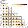 |
Fig. 4 Posterior distribution of the two-transit fit described in Sect. 3.2. |
| In the text | |
|
Fig. 5 Upper panel: TESS light curves of the two transits of DS Tuc A b and the adopted fit (black line). Lower panel: residuals of the light curves after the subtraction of the model. |
| In the text | |
|
Fig. 6 TESS undetrended light curves of the three transit events of DS Tuc A b, with the corresponding fit. |
| In the text | |
|
Fig. 7 Upper panel: correlation between HARPS bisector span and RVs obtained from the three different pipelines. Lower panels: timeseries of the RV residuals after removing the correlation from HARPS RVs (same colour-coding as for the pipelines). The solid lines represent the RV signal in the case of a planet with the same orbital elements as DS Tuc A b and a semi-amplitude corresponding to the mass upper limit estimated from the residuals (green line) and from empirical relation (blue line). |
| In the text | |
|
Fig. 8 Detection limits of the RV time series of DS Tuc A with a confidence level of 95%. |
| In the text | |
|
Fig. 9 Contrast plot in Δ Mag obtained around both stars of the binary for the 2004 and the 2009 observation. |
| In the text | |
|
Fig. 10 Mass detection limits expressed in MJup as a function of the separation from the stars expressed in au for both observing epochs and for both the stars of the binary. |
| In the text | |
|
Fig. 11 Summary of the FPP evaluation obtained with vespa. Acronyms of the false positive scenarios are defined in Sect. 4.3. |
| In the text | |
Current usage metrics show cumulative count of Article Views (full-text article views including HTML views, PDF and ePub downloads, according to the available data) and Abstracts Views on Vision4Press platform.
Data correspond to usage on the plateform after 2015. The current usage metrics is available 48-96 hours after online publication and is updated daily on week days.
Initial download of the metrics may take a while.