| Issue |
A&A
Volume 630, October 2019
Rosetta mission full comet phase results
|
|
|---|---|---|
| Article Number | A38 | |
| Number of page(s) | 9 | |
| Section | Planets and planetary systems | |
| DOI | https://doi.org/10.1051/0004-6361/201833544 | |
| Published online | 20 September 2019 | |
Unusually high magnetic fields in the coma of 67P/Churyumov-Gerasimenko during its high-activity phase
1
Institut für Geophysik und extraterrestrische Physik, Technische Universität Braunschweig, Mendelssohnstr. 3, 38106 Braunschweig, Germany
e-mail: This email address is being protected from spambots. You need JavaScript enabled to view it.
2
Jet Propulsion Laboratory, Pasadena, CA, USA
3
LPC2E, CNRS, Orléans, France
4
Institut für Weltraumforschung, Österreichische Akademie der Wissenschaften, Schmiedlstr. 6, Graz, Austria
5
Swedish Institute of Space Physics, PO Box 812, 981 28 Kiruna, Sweden
6
Swedish Institute of Space Physics, Angström Laboratory, Lägerhyddsvägen 1, Uppsala, Sweden
7
Southwest Research Institute, PO Drawer 28510, San Antonio, TX 78228-0510, USA
8
Mullard Space Science Laboratory, UCL Department of Space and Climate Physics, Holmbury St. Mary, Dorking, UK
Received:
1
June
2018
Accepted:
3
October
2018
Abstract
Aims. On July 3, 2015, an unprecedented increase in the magnetic field magnitude was measured by the Rosetta spacecraft orbiting comet 67P/Churyumov-Gerasimenko (67P). This increase was accompanied by large variations in magnetic field and ion and electron density and energy. To our knowledge, this unusual event marks the highest magnetic field ever measured in the plasma environment of a comet. Our goal here is to examine possible physical causes for this event, and to explain this reaction of the cometary plasma and magnetic field and its trigger.
Methods. We used observations from the entire Rosetta Plasma Consortium as well as energetic particle measurements from the Standard Radiation Monitor on board Rosetta to characterize the event. To provide context for the solar wind at the comet, observations at Earth were compared with simulations of the solar wind.
Results. We find that the unusual behavior of the plasma around 67P is of solar wind origin and is caused by the impact of an interplanetary coronal mass ejection, combined with a corotating interaction region. This causes the magnetic field to pile up and increase by a factor of six to about 300 nT compared to normal values of the enhanced magnetic field at a comet. This increase is only partially accompanied by an increase in plasma density and energy, indicating that the magnetic field is connected to different regions of the coma.
Key words: comets: individual: 67P/Churyumov-Gerasimenko / plasmas / magnetic fields / methods: data analysis
© ESO 2019
1 Introduction
The plasma environment at a comet is heavily dependent on the input solar wind conditions far upstream of the coma (Alfvén 1957; Nilsson et al. 2017; Goetz et al. 2017; Glassmeier 2017). The amount of mass-loading, that is, the incorporation of cometary ions in the solar wind flow, depends on solar wind parameters such as density, velocity, and magnetic field. As the comet approaches the Sun, the solar wind dynamic pressure and interplanetary magnetic field (IMF) magnitude increase slowly (Goetz et al. 2017), but so does the neutral outgassing rate of the nucleus as insolation increases. The neutral gas that is expelled from the nucleus is then ionized by processes such as photoionization and electron impact ionization. Therefore, the plasma density is controlled mostly by the intensity of the solar radiation and increases dramatically with decreasing distance between the comet and the Sun. The newly born ions present an obstacle to the solar wind and modify the plasma flow.
As the cometary ions are incorporated into the supersonic solar wind flow, the solar wind is slowed and eventually meets the conditions for the formation of a weak bow shock (Biermann et al. 1967; Koenders et al. 2013). The exact location of the bow shock then depends on the density of cometary ions and therefore on the neutral outgassing rate, as well as on the solar wind ram pressure. Behind the bow shock, the solar wind decelerates further and is deflected around the inner coma, whereas the IMF magnitude increases (pile-up) and the magnetic field starts to drape itself around the comet (Volwerk et al. 2014; Goetz et al. 2017). For sufficiently high gas production rates it may even reach deflections of up to 180°, and finally is entirely expelled from the inner coma (Behar et al. 2017, 2018). At this point, the cometary ions that have been picked up far upstream of the shock take over the main flow of plasma around the comet. At these gas production rates, it is also possible to observe an electron collisionopause (or exobase) in the inner coma (Coates & Jones 2009; Mandt et al. 2016). The innermost region in the plasma environment of the comet is the diamagnetic cavity, an entirely field-free region that is dominated by collisional ions and electrons (Neubauer 1987; Goetz et al. 2016a,b; Madanian et al. 2017; Henri et al. 2017). None of these boundaries is fixed in position, but they move according to gas production rate, as well as solar wind conditions. In particular, transient impulsive events in the solar wind of solar origin, such as interplanetary coronal mass ejections (ICMEs) and corotating interaction regions (CIRs), directly affect the cometary plasma properties.
Active regions (ARs) on the Sun are regions of multiple sunspots with complex photospheric and coronal magnetic fields. ARs are known to flare often, many times a day. With each major flare, an ICME is normally released. If the ICME has a speed in the interplanetary medium that is faster than the upstream in situ wave magnetosonic speed, a fast forward shock will form ahead of the ICME. Behind the shock will be a plasma sheath that contains heated and compressed slow solar wind plasma (Tsurutani et al. 1988). This sheath comes from a different solar source than the ICME. The amount of compression of the upstream slow solar wind plasma is directly related to the Mach number of the shock. The compression ratio is a maximum of 4 (Kennel et al. 1985; Tsurutani et al. 2008). When an interplanetary shock and its following sheath impinge upon a compressible object like the Earth’s magnetosphere, the high densities lead to magnetospheric compression.
High-speed solar wind streams emanate from coronal hole regions on the Sun. These are open magnetic field regions, and the streams have speeds of 750−800 km s−1. When the high-speed streams interact with low-speed (350−400 km s−1) solar wind, a CIR is formed (Smith & Wolfe 1976). The antisolar side of the CIR is composed of shocked and compressed slow solar wind plasma, and the solar side is composed of shocked and compressed high-speed solar wind plasmas. The two regions are separated by a tangential discontinuity (Pizzo 1985). At distances greater than ~ 1.5 AU from the Sun, CIRs are bounded by a forward shock at the antisolar side and by a reverse shock on the solar side. If a CIR that has both a forward and a reverse shock hits the Earth’s magnetosphere, the forward shock/sheath will compress the magnetosphere, and as the CIR reverse shock crosses it, the magnetosphere will decompress (Tsurutani et al. 2011).
The impact of CIRs and ICMEs on the cometary plasma environment has previously been investigated in situ only at comet 67P/Churyumov-Gerasimenko (67P) by Edberg et al. (2016a,b), Witasse et al. (2017), and Hajra et al. (2018). They found that CIRs and ICMEs both cause strong compressions of the plasma environment, resulting in higher magnetic fields and plasma densities. These fields and densities were accompanied by an increase in suprathermal electrons that may have been accelerated along the magnetic field lines. It was also found that electron impact ionization increased significantly during the event. For ICMEs it was observed that flux ropes exist in the compressed plasma at 67P. Energetic particle counts are also increased before the impact and culminate in a Forbush decrease (FD; Cane 2000) that begins about two hours before the signatures of the ICME are apparent in the plasma.
The Rosetta orbiter (Glassmeier et al. 2007a) spent two years orbiting comet 67P and continuously collected plasma data. One of the most striking events was an unusually high magnetic field of ~ 300 nT, an enhancement of about a factor of 50 compared to normal solar wind conditions and a factor of about six higher than normal for the piled-up magnetic field in the inner coma of 67P. We investigate possible triggers, especially those of solar wind origin. This is fairly difficult as the Rosetta mission did not include a solar wind monitor, which prevents an accurate determination of the upstream parameters. The only source of information are spacecraft near Earth and Mars. In particular, two additional sources for solar wind data were used, the OMNI dataset at Earth (King & Papitashvili 2005), and the MAVEN observations at Mars (Jakosky et al. 2015). To be usable at 67P, the propagation of the plasma through the solar system needs to be modeled accurately.
In this publication we describe the unusual measurements made on July 3, 2015, at comet 67P and search for the physical causes of this increase. Then we relate the significant changes in the plasma to structures in the coma and discuss the influence of the high field on them.
2 Instruments and data
We used all instruments in the Rosetta Plasma Consortium (RPC, Carr et al. 2007) the MAGnetometer (MAG, Glassmeier et al. 2007b), the Mutual Impedance Probe (MIP, Trotignon et al. 2007), the LAngmuir Probe (LAP, Eriksson et al. 2007), the Ion Composition Analyzer (ICA, Nilsson et al. 2007), and the Ion and Electron Sensor (IES, Burch et al. 2007). These instruments together are capable of measuring the magnetic field, electron and ion velocity space distribution functions with mass resolution, as well as plasma densities and temperature of electrons. However, there are a few caveats in using the data, which we briefly describe in the following.
First, the magnetic field, given in cometocentric solar equatorial coordinates (CSEQ), has been calibrated using observations in the diamagnetic cavity, which reduces the spacecraft influence to about 3 nT per field component. In the CSEQ system, the origin is at the nucleus, the x-axis points toward the Sun, the z-axis points out of the ecliptic, and the y-axis completes the right-handed coordinate system. ICA and IES have a limited field of view (90° × 360°) and may miss parts of the particle distribution functions. This is further complicated by the fact that the spacecraft is charged itself. For negative spacecraft potential, as it is observed in this event, slower ions are accelerated by the spacecraft potential and are detected at higher energies. This gives a skewed distribution function. Therefore, we used LAP spacecraft potential measurements to compare to the distribution functions.
MIP was operated in short Debye length (SDL) mode, with transmitters used in phase opposition (push–pull mode) during this event. In this mode, MIP is blind whenever the Debye length is larger than about one meter. For 5 eV electrons, this means that MIP cannot measure plasma densities below 300 cm−3. This lower limit can even increase for warmer electrons.
The lower densities may still be derived by using the LAP current and sweep-derived densities as well as MIP high densities to cross-calibrate and gain access to calibrated and high-time resolution LAP densities, in a way similar to what is described in Heritier et al. (2017). These densities were used here. We note that this cross-calibration assumes an isothermal hypothesis, so that in the presence of an electron temperature increase, as might be expected downstream of a shock, these cross-calibrated derived densities might be underestimated.
Additionally sampling rates vary drastically between instruments. IES has a sampling period of 256 s, ICA 4 s, MAG 0.05 s, and LAP 160 s for density and spacecraft potential and 0.017 s for the current. MIP has sample periods of a few seconds, but they are irregularly spaced, and in this specific case, are characterized by a larger amount of hot electrons. Only a reduced subset of the MIP spectra can be used to retrieve the electron density. ICA was not switched on for some time during the event.
As CIRs and ICMEs are accompanied by an increase in energetic particles, the Standard Radiation Monitor on board Rosetta (SREM, Evans et al. 2008) was used to provide context on these high energies. Rosina-COPS data are contaminated by wheel offloading and slews. Off-nadir pointing during the main event leads to very low densities, which are easily influenced by electron energies above 12 eV. This makes it impossible to obtain reliable neutral density measurements for this event, therefore we omitted these observations from the analysis.
We used observations made on July 3, 2015. At this time, the spacecraft was 180 km away from the nucleus and orbited at the terminator, and the comet was 1.3 AU away from the Sun, fairly close to perihelion (1.24 AU). According to Hansen et al. (2016), this corresponds to a water-outgassing rate of 5.8 × 1027 s−1. With these conditions, the spacecraft was located in the innermost part of the coma, far downstream of an undetected bow shock.
We used several observations in the solar system to provide context for the solar wind at 67P. STEREO data were not available for the time interval, but SOHO was observing the Earthward side of the Sun. MAVEN was in orbit around Mars and taking full particle distributions (SWIA) and observing the magnetic field (MAG). The solar wind parameters were determined using the method described by Halekas et al. (2017). The OMNI dataset was used to access the solar wind conditions at Earth. In an attempt to tie all observation points together, we used ENLIL simulations that cover the Sun, Earth, 67P, and Mars (Odstrcil 2003).
3 Observations
Figure 1 shows the plasma parameters in the two hours around the onset of the main event. Here, the cone angle ξ and the clock angle χ are defined in the CSEQ system as follows:
 (1)
(1)
Thus, a sunward field would have a cone angle of 90° and a northward (along the z-axis) field has a clock angleof 90°. Before the onset, the magnetic field had magnitudes of around 50 nT and exhibited very little fluctuation. The predominant component was the anti-sunward x-component. The plasma density was below the cutoff of MIP, and the electron flux was low. IES barely detected significant ion fluxes, but ICA was able to detect the cometary ion flux. The ions were mostly found to be in the energy range of 20 − 80 eV, but becauseof the high time resolution mode of ICA at the time, energies above 100 eV were not sampled. IES did not detect any solar wind ions during this interval, but there was significant obstruction (indicated by the white space). LAP probe bias sweeps (not shown) indicate that the electron temperature was around 3− 8 eV. This type of plasma is very typical for near-perihelion conditions at comet 67P.
At 21:32:10, the magnetic field magnitude increased by a factor of 2 to approximately 100 nT. The field was still mostly anti-sunward for the next five minutes; the cone and clock angles were unchanged. At the same time, the electron flux and energy were significantly elevated and the electron energy was approximately twice as high, whereas fluxes increased by a factor of five. The ion flux in IES was only slightly elevated, whereas in ICA the ion energies reached the upper energy cutoff and fluxes increased by a factor of 2. The spacecraft potential became slightly more negative, consistent with the increased electron flux.
Five minutes after the initial onset, at 21:37:08, the magnetic field abruptly changed direction to slightly sunward, and the field was below 10 nT for 3 s, the cone and clock angle varied significantly, and the cone angle changed from 90° to 0°. These field fluctuations were accompanied by electron densities of 3000−7000 cm−3 and ion flux doubling. This increase was very focused on a population around 100 eV and seemed to match the ICA observations as well, where the cometary ion flux in a range around 80 eV increased by a factor of two. The spacecraft potential decreased further to − 16.8 V. This plasma density enhancement ended after several minutes at 21:41:24, when all parameters returned to the previous elevated values.
The next change occured at 22:06:18. The magnetic field suddenly changed direction, and the magnitude increased further to above 200 nT. The magnetic field also fluctuated heavily with ΔB∕B ≈ 1. These fluctuations were mostly due to clock angle and magnitude changes, as the cone angle remained stable at − 90°. The peak field value of ~ 300 nT was reached at 22:12:39, which corresponds well to the IES electron flux maximum. This was due to a tenfold increase in flux in the energy band around 10 eV. The electron and ion flux were higher than in the previous quiet time, and the spacecraft potential reached around − 13.6 V. Again, this was mostly due to a populationof ions of about 100 eV; during the magnetic field peak, there was also an enhancement of about 200 eV. It should be noted that there is a large discrepancy between the density estimates derived from the MIP and LAP sensors, which is most likely due toa variation in electron temperature. Considering the observed change in the MIP lower frequency detection threshold, we are able to derive the factor by which the electron temperature is likely to have increased compared to the low-density region: ~ 9. This matches the difference in MIP and LAP densities well: the LAP density peaks are about a factor of ~ 3 below the MIP density peaks. As the temperature scales with the square of the density, this also gives a factor of 9. If the temperature in the low-density region was 5 eV, this would result in an electron temperature of 45 eV in the high-density region.
This high-activity region ended at 22:36:00, when the field rotated again and became anti-sunward (cone angle 90°). The high level offluctuation ceased, and plasma density values returned to below the detection threshold. The ion fluxes also decreased again by a factor of two.
In general, the event can be divided into three regions. Region 0 is the undisturbed coma, with a low field magnitude and variability and a sunward direction. This is accompanied by low ion and electron densities and energies. Region 1 is then characterized by a higher magnitude field that remains stable in the sunward direction and still exhibits low variability. Densities and energies are increased but still low. Region 2 then shows a rotation of the field in the anti-sunward direction and extremely high power in the magnetic field power spectral density (not shown), as well as high particle densities and energies. We have chosen to focus on the shown interval because regions 1 and 2 reoccurred in the next hours, but with diminishing strength that did not add any new features in the plasma environment.
4 Discussion
4.1 Possible triggers
As shown in Goetz et al. (2017), the magnetic field magnitude in the inner coma is determined by the field magnitude and dynamic pressure of the solar wind. Therefore, it is advisable to search solar wind observations for an extreme event that could cause the effects on the cometary plasma described above. Two such events are CIRs and ICMEs. Both have been reported at 67P for other solar wind and outgassing conditions (Edberg et al. 2016a,b; Witasse et al. 2017) to have caused higher magnetic field magnitudes,increases in electron density and fluxes over all energies, as well as increases in solar wind and cometary ion fluxes. In at least one case the impact of an ICME was sufficient to move the solar wind ion cavity boundary so close to the nucleus that it was detectable by Rosetta.
We therefore used images taken of the Sun to determine whether there were any ICMEs in the one-week period before the detected impact at the comet. During that time there was only one such event, an ICME on the evening of July 1, 2015, observed by SOHO. A simple calculation shows that to reach the comet in time, the ICME would have to have an average velocity of well above 1000 km s−1 on average. Because ICMEs tendto slow down as they propagate into the solar system, we can assume even higher velocities at the Sun. Events with solar wind velocities of 1500 km s−1 at 1 AU are very rare, thus it seems unlikely (but not impossible) that this structure reached the comet in time (Tsurutani et al. 2003). To verify whether this ICME reached the comet, we used ENLIL simulations with the cone model1. Three snapshots of the simulation are shown in Fig. 2. The figure shows the plasma density scaled with distance, and it is immediately clear that the ICME, which is visible as a very small disturbance almost reaching Mercury in the middle panel, reaches the comet (right panel) on July 6, which is almost three days after the investigated event. Additionally, the velocity of the ICME was chosen to be very high (1200 km s−1), so that realistically, the ICME would arrive even later. Because of its configuration, it is also questionable if its angular extension was large enough to have a significant impact on the cometary environment at all. However, there are uncertainties in the ENLIL simulations and the observations of the CME footpoint at the Sun, which means that it is not possible to rule out this ICME as the trigger.
A second type of solar wind event that usually has high dynamic pressures is a CIR. The snapshots in Fig. 2 were chosen so that the edge of a high-density CIR was either at Earth (left), 67P (middle), or Mars (right). In the following we try to identify the exact trigger of the July 3 event based on observations at the comet.
Figure 3 shows the magnetic field magnitude, counts from the Rosetta radiation monitor for the time around the investigated event, and the magnetic field and dynamic pressure measured in the solar wind at Earth at the time that the CIR would have to pass Earth to reach 67P on July 3. We also checked MAVEN observations of the solar wind at Mars, but there are several possible high dynamic pressure events that coincide with the predicted arrival time of a CIR at comet 67P, and thus we have opted not to discuss these observations further as they are ambivalent and do not aid in identifying the trigger of the high magnetic field.
First, there is a data gap in the Rosetta measurements when the instrument was shut off as a result of operational constraints. The event was preceded by a smaller magnetic field magnitude increase on June 30, which was associated with a change in cone angle (not shown). The magnetic field direction and amplitude were usually very variable at the comet (Goetz et al. 2017), which was also the case for most of the interval shown here. Conversely, the field magnitude was more stable on July 5 and 6, which also corresponds to steady conditions in the direction of the field. On the evening of July 6, it returned to its usual variable state. Therefore, we constrain the event to the interval from June 30 to July 6 at the comet.
An additional point of reference can be the energetic particle measurements that were observed by the Rosetta radiation monitor. This has previously been used to identify ICME impacts by Witasse et al. (2017). We show three energy channels: TC1 has a lower threshold of 27 MeV, and TC3 and S33 have lower thresholds of 12 MeV for protons. For electrons, the thresholds are 2 MeV and 0.8 MeV for TC1 andTC3. S33 is not sensitive to electrons (Evans et al. 2008). The upper threshold is infinity for all channels. As we are only interested in a qualitative evaluation of the measurements, no fluxes were calculated. On the eve of July 1, a first indication of an increased flux was visible. This increase lasted for about half a day before fluxes returned to slightly above normal. Unfortunately, magnetic field measurements are not available for most of that time period, but neither MIP nor LAP measurements changed significantly. On the evening of July 3, the particle counts increased dramatically, reaching their well-defined peak at 20:06:35. This peak is not associated with any change in the plasma, but the background noise in IES increased. At the time when the discontinuities in the plasma occurred, the energetic particle counts abruptly decreased to slightly above normal, and by 06:00:00 on July 4, the measurements had returned to previous normal levels. These observations are consistent with the results published by Witasse et al. (2017) for a Forbush decrease during an ICME. In addition, the SREM observationsare not very typical for a CIR; these are usually accompanied by only marginal increases in energetic particles.
The increase in energetic particles before the actual event then could be related to magnetic connectivity. If the approaching shock front or high-density region were magnetically connected to the comet, high-energy electrons might travelfaster along the field lines than the movement of the shock. This would explain the gradual increase before the arrival of the plasma discontinuity. The peak in count rate is usually associated with shock acceleration, but this is not supported by the plasma measurements, as there is no change at that time. All SREM observations indicate that 67P might not have encountered a CIR, but an ICME. This could be associated with a coronal hole that was observed from Earth with the SOHO spacecraft until it rotated out of the field of view in late June. When the rotation of the Sun is accounted for, this coronal hole is approximately in the same section of the heliosphere as 67P, making it a candidate for an ICME propagating toward 67P. However, because STEREO was in conjunction with Earth and unable to send data, observations from that side of the Sun are not available.
Identifying the exact trigger of the plasma disturbance at 67P is essential because no solar wind observations are available at the comet. If this event was triggered by a CIR, the solar wind conditions are much more constrained because there are measurements at Earth and Mars from which the solar wind can be propagated. If it was caused by a singular event like an ICME, observations at other solar system bodies not in the direct path of the ICME cannot be used. All observations indicate that the solar wind event that caused the high magnetic field at the comet was an ICME. That said, Fig. 3a also shows that in addition to the investigated event, no unusual features in the magnetic field at the comet are detected. No other unusually high magnetic field events in the month surrounding the event have been registered, although there should be a CIR passing the comet at least once during that time. The impact of that CIR should then be visible, which is not the case. This leads us to speculate that the event that triggered the reaction of the cometary plasma was the CIR interacting with an ICME. This would explain all observations, plasma, magnetic field and energetic particles, but because there was no solar wind monitor at the comet, this is just conjecture at this point.
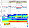 |
Fig. 1 Plasma parameters as observed by RPC during the main event. Panel a: magnetic field components and magnitude (black). Panel b: cone and clock angle of the magnetic field. Panel c: estimates of the plasma density from different instruments. IES observations are energy-summed flux adjusted to fit the scale. Panels d and e: electron and ion flux integrated over the entire field of view of IES. Panel f: spacecraft potential (multiplied by − 2 for clarity) derived from LAP sweeps and ion energy spectrogram measured by ICA. The vertical lines indicate the boundaries of the three plasma regions (indicated by numbers at the bottom). |
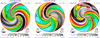 |
Fig. 2 Threesnapshots of the density output of the ENLIL simulation. The position of the comet is marked in gray (labeled “ROS”), and Mars is red, with Maven in orbit (labeled “MAV”). |
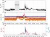 |
Fig. 3 Ten-day magnetic field magnitude measurements (panel a, averaged over 200 s in black) and energetic particle observations (panel b) made by Rosetta. Panel c: measurements of the solar wind at Earth from the OMNI dataset. The time axis was chosen so that the highest field and dynamic pressure coincide with the high-field event at Rosetta. This is to facilitate comparison of the structures. |
4.2 Reaction of the cometary plasma
4.2.1 Simple magnetic field model
Although we were unable to identify the physical cause of the event with certainty, we can estimate the reaction of the plasma environment to a CIR of the configuration that we infer from Earth-based observations. If our previous assumption of a combined CIR and ICME is correct, this should result in an underestimation of the solar wind density, velocity, and magnetic field as compared to a CIR-only case. Therefore, we would expect the reaction of the cometary environment to be stronger than estimated.
Goetz et al. (2017) presented a simple semi-analytical magnetic field model adapted from Galeev et al. (1985) that used a 1D magnetohydrodynamics (MHD) approach with a spacecraft that is confined to the Sun–comet line. It does not take into accountthe deflection of solar wind ions or the draping of the field. It was shown that despite the simplicity of the model, the output fit the magnetic field magnitude in the vicinity of the comet for suitable solar wind conditions reasonably well. Here, we use the model to estimate the impact that the high solar wind dynamic pressure hason the field in the inner coma. For this, we ran the model and extracted the magnetic field value at the radial distance of Rosetta, the result of which is shown in the left panel of Fig. 4. The model requires knowledge of the upstream dynamic and magnetic pressure in the solar wind, which is not available. However, as we have concluded in the previous section, the event at the comet may be related to the arrival of a CIR at Earth. Thus, we have chosen to infer the upstream solar wind conditions from the OMNI observations at Earth and propagated them to the comet using a simple Parker model. This approach does not include the influence of an ICME, as it is a transient event and is not observed at Earth, but it is still useful, as it gives us constraints on what the upstream solar wind conditions should be to produce such high magnetic fields at the comet.
The left-hand side of the figure shows that the general structure of the magnetic field in the model matches the observed field reasonably well. The maximum field magnitude in the model is 220 nT, which is still significantly lower than the maximum observed magnitude of ~ 300 nT (see Fig. 1a). At this point it is not possible to determine whether this is due to model uncertainties or upstreamcondition uncertainties. The solar wind values that produced the highest fields in the model were 25 nPa for the dynamic pressure and 0.25 nPa for the magnetic pressure. Although the magnetic and dynamic pressure may be higher individually, the importance here lies on the interplay of the two pressures.
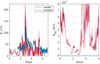 |
Fig. 4 Modeled magnetic field, bow shock position (red), and measured field and spacecraft position (blue). The input conditions for both models were calculated from OMNI solar wind observations using a Parker model for the propagation to the comet, and a gas production rate of Q = 5.8 × 1027 s−1. Day 0 corresponds to OMNI data from June 21, 2015. For readability, the magnetic field observations have been averaged over four minutes. |
4.2.2 Changing boundary positions
Solar wind protons were not detected in IES in this interval. As Rosetta was located in the solar wind-free region (Behar et al. 2017) for high gas production rates, this is not surprising. However, it also indicates that although the dynamic pressure in the solar wind is significantly enhanced, it is not enough to compress the bow shock to reach Rosetta. To ascertain this, we applied a simple mass-loading model to calculate the bow shock position (Biermann et al. 1967), again using the Earth observations as input. The model is a 1D gas dynamic approximation, thus it does not include magnetic fields and kinetic ions. It is therefore limited, and it was shown in Koenders et al. (2013) that it overestimates the bow shock distance compared to more sophisticated hybrid models at lower gas production rates and lower solar wind dynamic pressures. The result is shown on the right-hand side of Fig. 4. Most of the time, the bow shock is located well above 10 000 km, but for very high magnetic fields and thereby high solar wind dynamic pressures, the bow shock is pushed inward. The lowest bow-shock position estimate is still 1000 km, which is stillwell above the position of Rosetta. This estimate presents a lower boundary as the model does neither include asymmetric outgassing, that is, stronger outgassing on the sunward side of the comet, nor the fact that Rosetta is far from the subsolar point. Both these circumstances will push the bow shock position even farther from the nucleus than predicted (Huang et al. 2016).
According to Henri et al. (2017), the diamagnetic cavity is preferentially detected when the spacecraft is located close to the electron collisionopause, which is the approximate distance to the nucleus at which the electrons become collisional. It is defined as
 (2)
(2)
with σen the electron-neutral collision cross-section and un and Q the neutral gas velocity and production rate. Close to perihelion, almost all cavity crossings were found to be below 5 Le. During this unusual event, the neutral gas should not be affected by the higher magnetic fields and ion densities, which means that in the above equation, only σen is not constant. According to Itikawa & Mason (2005), the cross-section is electron energy dependent and decreases with increasing electron energy. The momentum transfer cross-section generally follows this trend as well, but has a secondary minimum at 2 eV and a secondary maximum at 10 eV. Normally, the electrons inside the diamagnetic cavity tend to be cold (Henri et al. 2017), with energies below 5 eV. It is plausible to assume that during this unusual event, with high densities, high magnetic fields, and high wave activity, that the electrons are heated. If the electrons inside the cavity are heated to below 15 eV, the electron collisionopause should expand as the cross-section increases. However, for electrons above 20 eV, the collisionopause shrinks as the cross-section decreases. With this the cavity boundary might either be moved inward or outward, depending on the electron energy inside the diamagnetic cavity. Unfortunately, it is not possible to distinguish between these two cases as measurements inside the diamagnetic cavity are not available for the studied time interval. The closest detection of the diamagnetic cavity was on July 7, 2015, at a distance of 150 km from the nucleus. At this point, the solar wind conditions had already returned to normal values and measurements are fundamentally different from the extraordinary circumstances studied here.
Another mechanism for the cavity formation was suggested by Cravens (1987), who assumed that the ion-neutral drag counter-balanced the magnetic field. This mechanism was tested by Timar et al. (2017) and found to accurately predict the diamagnetic cavity boundary distance in some cases. In this model, the diamagnetic cavity distance is proportional to 1∕B. Therefore, afivefold increase in the field as detected here would decrease the boundary distance by a factor of 5. Comparing this to the detection on July 7, this would mean a diamagnetic cavity size of 30 km. This is still significantly larger than the nucleus, and therefore even under the extreme solar wind conditions presented here, the solar wind magnetic field is unlikely to reach the surface of the comet.
4.2.3 Changes in cometary plasma
It is also interesting to note that there is a pronounced increase in the flux of electrons in the energy range of about 60 eV in the highest density region. Previously, this population was studied by Broiles et al. (2015) and Nemeth et al. (2016), the latter of whom found that this particular population vanishes when the spacecraft is inside, or very close to, the diamagnetic cavity. According to the former, this population is suprathermal and of solar wind origin. All of these observations point to the fact that the 60 eV population is most closely associated with the magnetic field. As the magnetic field increases, so does the electron density, and when the field vanishes inside the cavity, so do the electrons. A detailed statistical study of this phenomenon is underway. These results are consistent with what was observed by Edberg et al. (2016a,b), who also suggested that electrons are heated by the interaction with the solar wind and then move along the field lines.
There are five pronounced changes in magnetic field magnitude or direction, shown as vertical black lines in Fig. 1. Unfortunately, the Rankine–Hugoniot jump conditions could not be proven without reliable plasma velocities for any of these discontinuities. However, it is still possible to determine the surface normal, for which we used the average fields in the minute before and after the discontinuities. The times and characteristics of the five events indicated by the vertical black lines are listed in Table 1. The first discontinuity is characterized by a large increase in field and almost no change of direction. This, to a smaller degree, is also the case for the third. The second and fourth discontinuities seem to be best characterized by a rotational discontinuity: the field magnitude does not change significantly, whereas the direction reverses. The fourth discontinuity is especially remarkable, as the average magnitude does not change at all, whereas the direction reverses almost exactly. It should be pointed out that although the average magnitude does not change, the variability of the field does, giving the highest field shortly after the encounter of the fourth discontinuity. The last discontinuity is then a mixture of both rotational and compressional, but it should be noted that the magnetic field and densities start to slowly decrease even before the discontinuity is encountered. The direction of the normal seems to vary from region to region: the discontinuities bounding region 2 seem to be similar, that is, discontinuity two and three, and four and five are in similar planes. Only the first one is in an entirely different direction.
Goetz et al. (2017) found that the magnetic field variability, especially in a frequency band from 70 to 90 mHz, is an indicator of the neutral gas density and thereby also the ion density. The latter can be verified here as well; the high-density region also shows the highest values of the power spectral density.
It remains to discuss why the first increase in magnetic field at 21:32:10 is not accompanied by an increase in variability. One possibility for this would be that the high-density region is an effect of delayed ionization close to the nucleus. This would mean that the solar wind disturbance travels through the cometosheath to the inner, densest part of the coma and the high-energy electrons contribute significantly to additional electron impact ionization. The newly generated ions then travel outward to eventually reach Rosetta. However, this cannot be the case here, because then we would expect this increase in density to be permanent, which it is not, as region 2 reoccurs at least once.
Unfortunately, the exact amount of additional ionisation cannot be assessed, as neutral gas density observations are lacking for this event. They are fundamental for calculating the electron impact ionization (Vigren & Galand 2013).
A compression region at a CIR streaming interface could be the reason for the delayed increase. This might account for the delay, if the first shock corresponds to the forward wave front and the increase in density to the streaming interface. Thus, it is impossible to determine whether the delay is due to an internal change in the coma, such as increased ionization, or is due to an external trigger like the structure of the CIR.
Edberg et al. (2016a) found flux rope signatures in the magnetic field after the ICME impact and speculated that this might be due to reconnection in the inner coma. Therefore, we also searched for flux rope signatures. After determining the minimum variance direction with a minimum variance analysis (MVA, Sonnerup & Cahill 1967), we searched for a rotation in the magnetic field pointing in the maximum and medium variance direction. Surprisingly, no such structures were found after the high field event. This is unexpected, because the reconnection that was speculated on by Edberg et al. (2016a) should take place in the inner coma, where Rosetta was located during this event. Additionally, we find flux-rope-type structures in large numbers in the undisturbed plasma before and after the impact. Therefore, it seems as if flux-rope structures are a feature of the normal plasma at 67P and are not associated with the impact of an ICME in this case. A more detailed study of this is in preparation.
It is clear from these observations that there are fundamentally three regions in the interaction region around the event. We present two explanations for this: magnetic connectivity, and the structure of the solar wind.
First, the two regions after the shock impact have oppositely directed magnetic fields, meaning that in one instance, the field is mainly in the + x direction and in the other in the − x direction. It stands to reason, then, that the magnetic field is connected to different regions in the inner coma. Along the field line, the plasma can travel more freely, an effect that is often referred to as magnetic connectivity. In this instance, the magnetic field connects the spacecraft to a lower density region first and then to a high-density region. This idea assumes that the magnetic field in the solar wind also has different orientations that are then draped around the nucleus.
Second, the structure could be an intrinsic solar wind structure that propagates into the cometary environment and has higher densities from the start. These are then compressed. The fact that region 2 reoccurs speaks against this idea, as it is not obvious whythe solar wind structures should have such a nested configuration. It is certainly not visible in the observations at Earth. Additionally, the plasma seems already to be returning to normal values in the second region 2, which indicates that the solar wind event is already on its trailing edge. Concurrent with Mandt et al. (2016), the high-density region could also be a fixed structure in the plasma environment of the comet that moves back and forth above the spacecraft.
Discontinuity parameters.
5 Conclusions
We reported on the measurement of the highest magnetic fields ever measured at a comet and the associated plasma structures. In general, the results are consistent with previous findings and may be summarized as follows:
-
We find that the high field is caused by unusually high solar wind dynamic and magnetic pressure.
-
Based on observations at Earth, Mars, and comet 67P as well as observations of the Sun, we identify a CIR and an ICME aspossible triggers, raising the possibility that an interaction of both structures is responsible for the unusually high field.
-
A well-distinguished Forbush decrease is associated with the field structures. The highest count in energetic particles is about two hours before the event.
-
Three interaction regions are identified: the normal regime before the impact, a high-field regime, and a high-field or high-density regime. It is most likely that these are a result of the magnetic field connecting to different regions of the plasma environment of the comet.
-
In the high-density region, the suprathermal electron population increases significantly. This also implies that electron impact ionization is increased, but this could not be proven due to lack of data.
-
The simple model produces bow shock distances that are still greater than the cometocentric distance of the spacecraft. This is consistent with the non-observation of solar wind protons in the plasma during this event.
This study adds to previous results by investigating the cometary plasma reaction to high solar wind dynamic pressure events at high gas production rates. All features of the undisturbed plasma at perihelion are enhanced by the unusual solar wind conditions. However, more observations and simulations are needed to clarify the exact nature of the changes.
Acknowledgements
The RPC-MAG data will be made available through the PSA archive of ESA and the PDS archive of NASA. Rosetta is a European Space Agency (ESA) mission with contributions from its member states and the National Aeronautics and Space Administration (NASA). The work on RPC-MAG was financially supported by the German Ministerium für Wirtschaft und Energie and the Deutsches Zentrum für Luft- und Raumfahrt under contract 50QP 1401. We are indebted to the whole of the Rosetta Mission Team, SGS, and RMOC for their outstanding efforts in making this mission possible. We acknowledge the staff of CDDP and IC for the use of AMDA and the RPC Quicklook database (provided by a collaboration between the Centre de Données de la Physique des Plasmas, supported by CNRS, CNES, Observatoire de Paris and Université Paul Sabatier, Toulouse and Imperial College London, supported by the UK Science and Technology Facilities Council). Portions of this work were performed at the Jet Propulsion Laboratory, California Institute of Technology under contract with NASA. We acknowledge use of NASA/GSFC’s Space Physics Data Facility’s OMNIWeb (or CDAWeb or ftp) service, and OMNI data. Simulation results have been provided by the Community Coordinated Modeling Center at Goddard Space Flight Center through their public Runs on Request system (http://ccmc.gsfc.nasa.gov). The ENLIL Model was developed by D. Odstrcil at the University of Boulder at Colorado. A.W. acknowledges support from the STFC consolidated grant to UCL-MSSL ST/N000722/1. The authors would like to acknowledge ISSI for the great opportunity it offered for very valuable discussions on this topic as part of the International Team “Plasma Environment of comet 67P after Rosetta”.
References
- Alfvén, H. 1957, Tellus, 9 [Google Scholar]
- Behar, E., Nilsson, H., Alho, M., Goetz, C., & Tsurutani, B. 2017, MNRAS, 469, 396 [Google Scholar]
- Behar, E., Tabone, B., Saillenfest, M., et al. 2018, A&A, 620, A35 [Google Scholar]
- Biermann, L., Brosowski, B., & Schmidt, H. U. 1967, Sol. Phys., 1, 254 [NASA ADS] [CrossRef] [Google Scholar]
- Broiles, T. W., Burch, J. L., Clark, G., et al. 2015, A&A, 583, A21 [NASA ADS] [CrossRef] [EDP Sciences] [Google Scholar]
- Burch, J. L., Goldstein, R., Cravens, T. E., et al. 2007, Space Sci. Rev., 128, 697 [NASA ADS] [CrossRef] [Google Scholar]
- Cane, H. V. 2000, Space Sci. Rev., 93, 55 [NASA ADS] [CrossRef] [Google Scholar]
- Carr, C., Cupido, E., Lee, C. G. Y., et al. 2007, Space Sci. Rev., 128, 629 [NASA ADS] [CrossRef] [Google Scholar]
- Coates, A. J., & Jones, G. H. 2009, Planet. Space Sci., 57, 1175 [NASA ADS] [CrossRef] [Google Scholar]
- Cravens, T. E. 1987, Adv. Space Res., 7, 147 [NASA ADS] [CrossRef] [Google Scholar]
- Edberg, N. J. T., Alho, M., André, M., et al. 2016a, MNRAS, 462, S45 [CrossRef] [Google Scholar]
- Edberg, N. J. T., Eriksson, A. I., Odelstad, E., et al. 2016b, J. Geophy. Res. (Space Phys.), 121, 949 [NASA ADS] [CrossRef] [Google Scholar]
- Eriksson, A. I., Boström, R., Gill, R., et al. 2007, Space Sci. Rev., 128, 729 [NASA ADS] [CrossRef] [Google Scholar]
- Evans, H. D. R., Bühler, P., Hajdas, W., et al. 2008, Adv. Space Res., 42, 1527 [NASA ADS] [CrossRef] [Google Scholar]
- Galeev, A. A., Cravens, T. E., & Gombosi, T. I. 1985, ApJ, 289, 807 [NASA ADS] [CrossRef] [Google Scholar]
- Glassmeier, K.-H., Boehnhardt, H., Koschny, D., Kührt, E., & Richter, I. 2007a, Space Sci. Rev., 128, 1 [NASA ADS] [CrossRef] [Google Scholar]
- Glassmeier, K.-H., Richter, I., Diedrich, A., et al. 2007b, Space Sci. Rev., 128, 649 [NASA ADS] [CrossRef] [Google Scholar]
- Glassmeier, K.-H. 2017, Philos. Trans. R. Astron. Soc. A, 375, 20160256 [Google Scholar]
- Goetz, C., Koenders, C., Hansen, K. C., et al. 2016a, MNRAS, 462, S459 [Google Scholar]
- Goetz, C., Koenders, C., Richter, I., et al. 2016b, A&A, 588, A24 [Google Scholar]
- Goetz, C., Volwerk, M., Richter, I., & Glassmeier, K.-H. 2017, MNRAS, 469, S268 [CrossRef] [Google Scholar]
- Hajra, R., Henri, P., Myllys, M., et al. 2018, MNRAS, 480, 4544 [Google Scholar]
- Halekas, J. S., Ruhunusiri, S., Harada, Y., et al. 2017, J. Geophys. Res. (Space Phys.), 122, 547 [NASA ADS] [CrossRef] [Google Scholar]
- Hansen, K. C., Altwegg, K., Berthelier, J.-J., et al. 2016, MNRAS, 462, S491 [Google Scholar]
- Henri, P., Vallières, X., Hajra, R., et al. 2017, MNRAS, 469, S372 [Google Scholar]
- Heritier, K. L., Henri, P., Vallières, X., et al. 2017, MNRAS, 469, S118 [CrossRef] [Google Scholar]
- Huang, Z., Tóth, G., Gombosi, T. I., et al. 2016, J. Geophys. Res. (Space Phys.), 121, 4247 [NASA ADS] [CrossRef] [Google Scholar]
- Itikawa, Y., & Mason, N. 2005, J. Phys. Chem. Ref. Data, 34, 1 [NASA ADS] [CrossRef] [Google Scholar]
- Jakosky, B. M., Lin, R. P., Grebowsky, J. M., et al. 2015, Space Sci. Rev., 195, 3 [NASA ADS] [CrossRef] [Google Scholar]
- Kennel, C. F., Edmiston, J. P., & Hada, T. 1985, Geophysical Monograph Series, 34 (Washington DC: AGU), 1 [Google Scholar]
- King, J. H., & Papitashvili, N. E. 2005, J. Geophys. Res. (Space Phys.), 110, A02104 [NASA ADS] [CrossRef] [Google Scholar]
- Koenders, C., Glassmeier, K.-H., Richter, I., Motschmann, U., & Rubin, M. 2013, Planet. Space Sci., 87, 85 [NASA ADS] [CrossRef] [Google Scholar]
- Madanian, H., Cravens, T. E., Burch, J., et al. 2017, AJ, 153, 30 [Google Scholar]
- Mandt, K. E., Eriksson, A., Edberg, N. J. T., et al. 2016, MNRAS, 462, S9 [NASA ADS] [CrossRef] [Google Scholar]
- Nemeth, Z., Burch, J., Goetz, C., et al. 2016, MNRAS, 462, S415 [Google Scholar]
- Neubauer, F. M. 1987, A&A, 187, 73 [NASA ADS] [Google Scholar]
- Nilsson, H., Lundin, R., Lundin, K., et al. 2007, Space Sci. Rev., 128, 671 [NASA ADS] [CrossRef] [Google Scholar]
- Nilsson, H., Wieser, G. S., Behar, E., et al. 2017, MNRAS, 469, S252 [CrossRef] [Google Scholar]
- Odstrcil, D. 2003, Adv. Space Res., 32, 497 [CrossRef] [Google Scholar]
- Pizzo, V. J. 1985, Geophysical Monograph Series, 35 (Washington DC: AGU), 51 [Google Scholar]
- Smith, E. J., & Wolfe, J. H. 1976, Geophys. Res. Lett., 3, 137 [NASA ADS] [CrossRef] [Google Scholar]
- Sonnerup, B. U. O., & Cahill, Jr. L. J. 1967, J. Geophys. Res., 72, 171 [NASA ADS] [CrossRef] [Google Scholar]
- Timar, A., Nemeth, Z., Szego, K., et al. 2017, MNRAS, 469, S723 [Google Scholar]
- Trotignon, J. G., Michau, J. L., Lagoutte, D., et al. 2007, Space Sci. Rev., 128, 713 [NASA ADS] [CrossRef] [Google Scholar]
- Tsurutani, B. T., Gonzalez, W. D., Tang, F., Akasofu, S. I., & Smith, E. J. 1988, J. Geophy. Res., 93, 8519 [NASA ADS] [CrossRef] [Google Scholar]
- Tsurutani, B. T., Gonzalez, W. D., Lakhina, G. S., & Alex, S. 2003, J. Geophy. Res. (Space Phys.), 108, 1268 [Google Scholar]
- Tsurutani, B. T., Echer, E., Guarnieri, F. L., & Kozyra, J. U. 2008, Geophys. Res. Lett., 35 [Google Scholar]
- Tsurutani, B. T., Lakhina, G. S., Verkhoglyadova, O. P., et al. 2011, J. Atmos. Sol. Terr. Phys., 73, 5 [NASA ADS] [CrossRef] [Google Scholar]
- Vigren, E., & Galand, M. 2013, ApJ, 772, 33 [Google Scholar]
- Volwerk, M., Glassmeier, K. H., Delva, M., et al. 2014, Ann. Geophys., 32, 1441 [NASA ADS] [CrossRef] [Google Scholar]
- Witasse, O., Sánchez-Cano, B., Mays, M. L., et al. 2017, J. Geophy. Res. (Space Phys.), 122, 7865 [Google Scholar]
The full heliospheric simulation results may be found at http://ccmc.gsfc.nasa.gov under run number Charlotte_Goetz_062416_SH_1.
All Tables
All Figures
|
Fig. 1 Plasma parameters as observed by RPC during the main event. Panel a: magnetic field components and magnitude (black). Panel b: cone and clock angle of the magnetic field. Panel c: estimates of the plasma density from different instruments. IES observations are energy-summed flux adjusted to fit the scale. Panels d and e: electron and ion flux integrated over the entire field of view of IES. Panel f: spacecraft potential (multiplied by − 2 for clarity) derived from LAP sweeps and ion energy spectrogram measured by ICA. The vertical lines indicate the boundaries of the three plasma regions (indicated by numbers at the bottom). |
| In the text | |
|
Fig. 2 Threesnapshots of the density output of the ENLIL simulation. The position of the comet is marked in gray (labeled “ROS”), and Mars is red, with Maven in orbit (labeled “MAV”). |
| In the text | |
|
Fig. 3 Ten-day magnetic field magnitude measurements (panel a, averaged over 200 s in black) and energetic particle observations (panel b) made by Rosetta. Panel c: measurements of the solar wind at Earth from the OMNI dataset. The time axis was chosen so that the highest field and dynamic pressure coincide with the high-field event at Rosetta. This is to facilitate comparison of the structures. |
| In the text | |
|
Fig. 4 Modeled magnetic field, bow shock position (red), and measured field and spacecraft position (blue). The input conditions for both models were calculated from OMNI solar wind observations using a Parker model for the propagation to the comet, and a gas production rate of Q = 5.8 × 1027 s−1. Day 0 corresponds to OMNI data from June 21, 2015. For readability, the magnetic field observations have been averaged over four minutes. |
| In the text | |
Current usage metrics show cumulative count of Article Views (full-text article views including HTML views, PDF and ePub downloads, according to the available data) and Abstracts Views on Vision4Press platform.
Data correspond to usage on the plateform after 2015. The current usage metrics is available 48-96 hours after online publication and is updated daily on week days.
Initial download of the metrics may take a while.