© ESO 2019

1. Introduction

Astrometry is a powerful technique for detecting companions to the nearby ultracool dwarfs by monitoring the induced reflex motion, provided that a measurement precision better than 1 mas can be achieved. For ground-based observations, this requires the use of 8–10 m telescopes and good observing conditions. For targets near the Galactic plane, where a large number of reference stars is available, and 0.4″ seeing, the initial estimates of Lazorenko & Lazorenko (2004) indicated an achievable astrometric accuracy of 0.01–0.06 mas for faint stars. With the Very Large Telescope (VLT) camera FORS2 (Appenzeller et al. 1998) we demonstrated a single-epoch astrometric accuracy close to 0.1 mas for 15–20 mag stars and 0.6″ atmospheric seeing (Lazorenko et al. 2009; Sahlmann et al. 2014; Lazorenko et al. 2014; Lazorenko & Sahlmann 2017). This accuracy is sufficient to detect and characterize the orbits of Jupiter-mass companions to nearby ultracool dwarfs. With this purpose, we initiated an astrometric planet search around 20 ultracool dwarfs in 2011 (Sahlmann et al. 2015a,b).

The further accuracy improvement beyond 0.1 mas, needed for the detection of Neptune- and lower-mass companions to ultracool dwarfs, is restrained by fundamental limits on the precision of photocenter determination, the atmospheric image motion caused by turbulence in the upper atmospheric layers, and by systematic errors of instrumental origin. It is expected that in the near future the achievable astrometric accuracy will be improved to 0.01–0.05 mas on 30 m class telescopes such as the European Extremely Large Telescope (ELT), primarily due to the use of adaptive optics, better signal-to-noise ratio in the stellar images, and general performance improvements of the cameras (Davies et al. 2010; Rodeghiero et al. 2018; Pott et al. 2018).

The CCD detectors in most cameras of large telescopes are formed as mosaics of CCD chips allowing for a wide field of view (FoV). However, this structure of detectors potentially affects geometric stability of the compound image when the mounting of the CCDs is not sufficiently rigid. The first evidence of the displacements in the FORS2 CCD mosaic were detected by Lazorenko et al. (2014; hereafter Paper I) from the analysis of two years of data. At that time, we discovered a relative chip motion (RCM) in the two-chip CCD mosaic with an amplitude of 0.001–0.010 px, or 0.1–1 mas. In one peculiar case, we detected a shift of nearly 0.02–0.05 px or 3–6 mas. These amplitudes were small but exceeded the astrometric accuracy of FORS2 by a factor of 10.

Relative chip motion was observed for cameras on board the Hubble Space Telescope (Anderson & King 2003, Sect. 6)¹ with an amplitude of up to 3 px = 120 mas over ∼10 years. More recently, Bernstein et al. (2017) analyzed the stability of the CCD chip array of the Dark Energy Camera (DECam) and discovered surprisingly large RCM with an amplitude of 0.4 px = 100 mas occurring over only 2 weeks.

In this paper, we use newly obtained series of FORS2 observations to characterize the instability of its detector chips. We also predict how these instrumental errors can affect the astrometric performance of FORS2 and other telescopes.

2. Observational data

This study is based on observations of N_dw = 20 ultracool dwarfs obtained with the FORS2 camera of the VLT. The program of observations, reduction methods, and the first results obtained from observations in 2010–2013 are described in Sahlmann et al. (2014) and Paper I. We monitored all targets during two visibility periods, but for targets with suspected orbital signals, we followed up with additional observations. As a consequence, six fields were observed over one to one and a half years, seven fields were observed for three years, and the seven remaining fields were monitored over six to seven years. We refer to the corresponding data as the short-, medium-, and long-duration datasets.

The FORS2 detector has an exchangeable blue (E2V) and red (MIT) sensitive detector pair. We used FORS2 only in its standard configuration with an MIT detector. This detector is a mosaic of two CCD chips. With the 2 × 2 binned read-out mode we used, they are 2k × 1k pixel arrays with pixel sizes of 30 μm. The upper chip 1 and the lower chip 2 are mounted with a small gap of ∼480 μm (∼16 binned pixels). Observations were obtained with a high-resolution collimator that produces an angular pixel scale of 126.1 mas pixel. Every observation “epoch” consists of a series of 30–100 images. For the different sky fields we obtained N_e = 10…23 epochs of observations.

In every image, we measured 500–1500 star photocenters x, y of i = 1…N unsaturated reference stars. The following reduction proceeded in a coordinate system whose axes X, Y are oriented along RA, Dec. For convenience, the row y = 1000 px was aligned with the upper edge of the gap between the chips (a lower edge of the upper chip 1), thus y <  1000 px identifies stars in the bottom chip 2, and y >  1000 px corresponds to the upper chip 1.

3. Basic astrometric reduction

The observations are reduced with differential astrometric techniques as previously reported (Lazorenko et al. 2009; Paper I), where we use the effective filtration of the atmospheric image motion by the large ground-based telescope (Lazorenko & Lazorenko 2004). This technique requires a circular reference field, and the best performance is achieved at its center. For this reason, the reference field is centered on the target object. We take into consideration that the atmospheric image motion variance increases with the reference field size R while the reference frame noise decreases with R. Therefore, there is some optimal radius R_opt at which the sum of these error components is smallest. Its value is determined numerically and is 400–800 px (1–2′ for FORS2), which is typical for the sky fields near the Galactic plane.

A list of the variables that are most frequently used in the paper along with a short description is given in Table 1.

3.1. Astrometric model

All measured stars (except for the target object) are used as references to provide the best information on the geometric distortion Φ(x, y) of the field caused both by the instability of the telescope optics and its adjustment, and by the image motion. Its spatial power density is represented by an infinite expansion into series of even integer powers k = 2, 4, … in the domain of the spatial frequencies, where k is the modal index, and the mode amplitude decreases rapidly with increasing k. Over the CCD space (x, y), the image motion causes deformations of the frame of reference stars that are modeled by an expansion into a series of basic functions f_i, 1 = 1, f_i, 2 = x_i, f_i, 3 = y_i, $f_{i,4}=x_i^2\dots$ which are full bivariate polynomials of x, y and whose number N′ = 1…k(k + 2)/8 depends on k. The use of functions Φ(x, y) in the reduction model removes all first 1…k/2 − 1 modes of the image motion spectrum. Usually, k is between 4 and 16, and for this study, we set k = 10, which leads to the most stable solution. The function ${\mathrm{\Phi }}_m^x(x,\mathit{y})=\sum _{\mathit{w}=1}^{N\prime }{c}_{\mathit{w},m}^x{f}_{i,\mathit{w}}$ therefore includes N′×M coefficients $c_{\mathit{w},m}^x$ that model geometric distortions to the fourth power of x, y at the exposure number m = 1…M. Similarly, ${\mathrm{\Phi }}_m^y(x,y)$ models geometric distortions along the Y-axis through the coefficients $c_{\mathit{w},m}^{\mathit{y}}$.

The displacement of some star i photocenter (either the target or reference star) from its initial position x_i, 0, y_i, 0 in the reference frame (exposure m = 0) to x_i, m, y_i, m in exposure m is caused by intrinsic (proper motion, parallax) and atmospheric (refraction) motion. We model it with s = 1…S astrometric parameters ξ_i, s: the offsets to the positions Δx_0, i, Δy_0, i, proper motion μ_x, i, μ_y, i, relative parallax ϖ, and two atmospheric differential chromatic parameters ρ and d, that is, S = 7. The corresponding displacement is ${\varphi }_m^x(\xi ,{\nu }^x)=\sum _{s=1}^S{\xi }_{i,s}{\nu }_{s,m}^x$ and ${\varphi }_m^{\mathit{y}}(\xi ,{\nu }^{\mathit{y}})=\sum _{s=1}^S{\xi }_{i,s}{\nu }_{s,m}^{\mathit{y}}$, where ν^x, ν^y are S × M coefficients (time t, parallax factors Π, etc.) valid at the time of exposure t_m for the measurements along X or Y. In particular, ${\varphi }_{m,i}^x(\xi ,{\nu }^x)=\mathrm{\Delta }{x}_{0,i}+{\mu }_{x,i}{t}_m+{\varpi }_{x,i}{\mathrm{\Pi }}_{x,i,m}-\rho f{1}_{x,m}-df{2}_{x,m}$, where functions f1, f2 depend on zenith distance, parallax angle, temperature, and pressure (Sahlmann et al. 2014).

All ξ values are determined as free model parameters. Alternatively, the reduction model can be significantly simplified if some ξ values are taken from the external sources. In particular, Gaia DR2 (Lindegren et al. 2018) provides proper motions with standard uncertainties of 0.08–0.16 mas yr⁻¹ for G = 16–17 mag stars. For our targets of comparable magnitudes with a time base of about 1.4 yr, the accuracy of FORS2 proper motions is 0.10 mas yr⁻¹ (Paper I), which improves to 0.01–0.03 mas yr⁻¹ for the objects monitored over 5–7 yr. Because the accuracy of differential FORS2 proper motions and parallaxes is currently better, we do not use DR2 as an external source of ξ values at this time. However, we use Gaia DR2 as an astrometric flat-field calibrator, see Sect. 6.2. The differential chromatic refraction (DCR) parameters ρ, d can be constrained using stellar spectra (e.g., Garcia et al. 2017), however for field stars these are usually unavailable.

The measured displacement of a star from the initial position x₀, y₀ is described by the sum of functions Φ(x, y) and ϕ(ξ, ν), or

$$\begin{array}{c}\hfill \begin{array}{c}\sum _{w=1}^{N^{\prime }}{c}_{w,m}^x{f}_{i,w}+{\sum }_{s=1}^S{\xi }_{i,s}{\nu }_{s,m}^x+H_m^{x}U(y)+{\delta }_{i,m}^x=x_{i,m}-x_{i,0},\hfill \\ \sum _{w=1}^{N^{\prime }}{c}_{w,m}^y{f}_{i,w}+{\sum }_{s=1}^S{\xi }_{i,s}{\nu }_{s,m}^y+H_m^{y}U(y)+{\delta }_{i,m}^y=y_{i,m}-y_{i,0}.\hfill \end{array}\end{array}$$(1)

This system is solved using reference stars i ∈ ω, where ω is the reference space that includes either chip 1 only or stars of both chips within R_opt distance from the target. Equation (1) is solved with the weights P_i, m assigned according to the measurement uncertainties σ_i, m of the star i in the frame m. In the context of this investigation, additional terms $H_m^x$, $H_m^{\mathit{y}}$ are included as the potential displacement of chip 2 relative to chip 1 along the coordinate axes in exposure m. In the primary astrometric reduction, the solution of Eq. (1) is derived assuming H = 0, and later, during the second phase of the investigation, the terms H_m are extracted by analyzing the model residuals ${\delta }_{i,m}^x$, ${\delta }_{i,m}^{\mathit{y}}$ and the peculiar properties of the ξ parameters. The step function U(y)

$$\begin{array}{c}\hfill \begin{array}{ccc}& U(y)=1\mathrm{if}y<1000\hfill & \hfill (lowerchip2)\\ \hfill & U(y)=0\mathrm{if}y>1000\hfill & \hfill (upperchip1)\end{array}\end{array}$$(2)

is introduced to limit the application of the H function to one chip only. The system Eq. (1) is solved with S × N′ conditions

$$\begin{array}{c}\hfill {\displaystyle \sum _{i\in {\omega }^{\ast }}}{\xi }_{i,s}{\overline{P}}_i{f}_{i,w}(x_i,y_i)=0,s=1\dots S,w=1\dots N^{\prime }\end{array}$$(3)

on the parameters ξ in the normalizing parameter space ω^*, which does not necessarily coincide with ω. When s is fixed, Eq. (3) can be understood as the formal expression of the fact that the least-squares residuals (which are recognized here as ξ_i) are orthogonal to each of w = 1…N′ basic functions f_w of some conditional system of i = 1…N measurements obtained with the weights ${\overline{P}}_i$. In this interpretation, the corresponding system of conditions is ${\xi }_{i,s}^{\mathrm{abs}}=\sum _{\mathit{w}=1}^{N\prime }{c}_{\mathit{w},s}^{\ast }{f}_{i,\mathit{w}}$, where ξ^abs are the parameters given in some external (e.g., absolute) system. Consequently, ${\xi }_{i,s}={\xi }_{i,s}^{\mathrm{abs}}-\sum _{\mathit{w}=1}^{N\prime }{c}_{\mathit{w},s}^{\ast }{f}_{i,\mathit{w}}$ represents the fit residuals (Lazorenko et al. 2009). This establishes the relationships between the system of relative parameters ξ, the absolute parameters ξ^abs, fit constants c^*, the weights ${\overline{P}}_i$, and the functions f_w.

One property of the derived parameters ξ is that the weighted sum of differential proper motions is zero, that they do not change systematically across the FoV, and that they do not correlate with x, y, xy or any other function f_w, which is expressed by $\sum {\mu }_i{\overline{P}}_i=\sum {\mu }_i{\overline{P}}_i{x}_i=\sum {\mu }_i{\overline{P}}_i{\mathit{y}}_i=\dots \sum {\mu }_i{\overline{P}}_i{f}_{i,\mathit{w}}=0$. Equation (3) is applied with arbitrary weights ${\overline{P}}_i$ that define the system of relative parameters ξ. In practice, we set ${\overline{P}}_i=1$ for sufficiently bright stars and ${\overline{P}}_i=0$ for ∼10% for fainter reference stars to exclude wildly scattered values ξ of these stars. For the standard astrometric reduction, we usually set ω^* = ω, but in this investigation, ω^* space can be expanded over ω, see Table 2.

The model Eq. (1) with constraints Eq. (3) is solved iteratively as described in Lazorenko et al. (2009), in turn deriving c_w, m within each single image m at some fixed ξ_i, s. With these c_w, m, we then update ξ_i, s separately for each single reference star i. Here we omit the details of the reduction and note only that as soon as iterations converge and the geometric distortions Φ_m of each frame m are found, the ith star’s astrometric parameters ξ_i, s are derived from the subsystem of equations

$$\begin{array}{c}\hfill \begin{array}{c}{\sum }_s{\xi }_{i,s}{\nu }_{s,m}^x+{\delta }_{i,m}^x+H_m^{x}U(y)=V_{i,m}^x\hfill \\ {\sum }_s{\xi }_{i,s}{\nu }_{s,m}^y+{\delta }_{i,m}^y+H_m^{y}U(y)=V_{i,m}^y,\hfill \end{array}\end{array}$$(4)

where $V_{i,m}^x=x_i-x_{i,0}-{\mathrm{\Phi }}_m^x(x_i,{\mathit{y}}_i)$, and $V_{i,m}^{\mathit{y}}={\mathit{y}}_i-{\mathit{y}}_{i,0}-{\mathrm{\Phi }}_m^{\mathit{y}}(x_i,{\mathit{y}}_i)$ are the stellar displacements corrected for Φ_m. This system involves m = 1…M measurements of the star i and is solved considering both x and y data simultaneously, which also yields the residuals ${\delta }_{i,m}^x$, ${\delta }_{i,m}^{\mathit{y}}$. Because ${\nu }_{s,m}^x$, ${\nu }_{s,m}^{\mathit{y}}$ are the basic functions of the system Eq. (4) solved by the least-squares fit, the residuals ${\delta }_{i,m}^x$, ${\delta }_{i,m}^{\mathit{y}}$ are orthogonal to these functions. In particular, they should have no linear dependence on time. Similarly, the residuals ${\delta }_{i,m}^x$, ${\delta }_{i,m}^{\mathit{y}}$, which are orthogonal to the basic functions f_i, w of Eq. (1), should have no systematic trend along X or Y. The frame residuals of reference stars, converted into the epoch residuals ${\mathrm{\Delta }}_{i,\mathrm{e}}^x$ and ${\mathrm{\Delta }}_{i,\mathrm{e}}^{\mathit{y}}$, can display some correlation pattern that is caused by systematic errors, which provides useful information on these errors. In particular, the investigation of the epoch residuals derived under the assumption that H(t) = 0 allows us to reveal the time-dependent relative chip motion.

3.2. RF and CAL files

The principal results of the astrometric reduction are the parameters ξ_i, s and the epoch residuals ${\mathrm{\Delta }}_{\mathrm{e}}^x$, ${\mathrm{\Delta }}_{\mathrm{e}}^{\mathit{y}}$ derived for the star i that is the target object. In addition, we obtain the same quantities for every reference star within a circular reference field centered on the target. These data in 20 sky fields are referred to as the reference frame (RF) files. The uncertainties of the RF dataset change across the field and are smallest at its center. At the outer boundaries, the astrometric accuracy degrades because the uncertainty of the Φ(x, y) determination increases.

Stars in the RF files do not cover the full FoV for typical sizes of R_opt. For calibration purposes we need to know the astrometric parameters and the epoch residuals of all stars in the full FoV. We achieve this by repeating the basic reduction for each of i = 1…N field stars, setting it as the target object. The results are saved in the calibration (CAL) files that contain results for the single central star only. In CAL files the reference star data are disregarded because the precision is reduced. The CAL files include most stars in the FoV and therefore contain about three times more stars than RF files.

3.3. Response properties of the astrometric model

The model defined by Eqs. (1)–(3) can be treated as a filtering system that absorbs some part of a signal at its entrance because of the least-squares fit of data. Therefore we should not expect that the chip displacement H(t) that affects the measurements is fully reflected in the epoch residuals. We demonstrate this with the help of reference stars around the brown dwarf DENIS J125310.8−570924 (hereafter dw14), for which we obtained N_e = 23 epochs over about seven years. We introduced a step change U(y) = 1 in the measurements x_i, e obtained on 17 February 2012 and performed our reduction process. Figure 1 shows that the computed residuals differ significantly from the introduced step change. The residuals have a discontinuity at y = 1000 px with an offset amplitude of 1 between the chips. The scatter of individual ${\mathrm{\Delta }}_i^x$ values relative to their systematic change as a function of y is related to a weak dependence of ${\mathrm{\Delta }}_i^x$ on x, and a small asymmetry relative to the detector center y = 1000 px is due to the location of the reference field center ∼73 px off the gap between the chips.

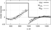Fig. 1. Simulation of the astrometric model response to a step change U(y) in the position of chip 2 for the example sky field of dw14 offset by 73 px from the detector center. Dots show the response in the epoch residuals ${\mathrm{\Delta }}_{i,\mathrm{e}}^x$ of reference stars, and the function WRF is the smoothed response in proper motions to the step change of proper motions of chip 2 stars. The function WCAL is the same, but for the reference stars distributed evenly over FoV.

The solid curves in Fig. 1 correspond to the systematic change of the residuals if the reduction is made with P_i, m = 1. The restriction Eq. (3) leads to ξ parameters that are orthogonal to the functions f with the weights ${\overline{P}}_i=1$, that is, the response characteristics of ξ and Δ_i derived with P_i, m = 1 are exactly equivalent. In this interpretation, solid curves represent the model response W_RF in ξ (e.g., in proper motions) to the step change of these parameters for all chip 2 stars by U(y). The response W_RF corresponds to RF files or to the proper motions of reference stars in a field centered at the target.

The dashed lines in Fig. 1 correspond to a reference field that is symmetric around the detector center y = 1000 px and with P_i, m = 1 set in Eq. (1). This option approximately corresponds to the averaging of response functions over many circular reference fields with centers that cover most of the FoV, and we therefore used it as the response function W_CAL for the CAL files. This function is nearly antisymmetric relative to y = 1000 px, where it is equal to ±0.5. Below we discuss the application of the response functions to the effects in the epoch residuals and in proper motions. The above examples demonstrate that a step signal U(y) is associated with a specific discontinuity pattern in the epoch residuals or proper motions.

4. Observational evidence of the chip motion

First evidence of the FORS2 chip mosaic instability was found in the epoch residuals of reference stars within the same reference field, but located in different chips (Paper I). As an example, Fig. 2 shows the residuals ${\mathrm{\Delta }}_{\mathrm{e}}^x$ in RA of stars in the sky field of dw14. The residuals are shown separately for the stars imaged in each chip and for a few bright stars only that were measured with a single-epoch uncertainty of 0.1–0.5 mas, or about 1–3 millipixels (mpx). These residuals do not show a linear trend in time because the astrometric model includes the proper motion as a model parameter. However, a significant time-dependent variation with opposite sign in both chips is evident.

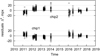Fig. 2. Epoch positional residuals ${\mathrm{\Delta }}_{\mathrm{e}}^x$ for bright reference stars imaged close to the chip gap in the sky field of dw14. The residuals are shown separately for stars in chip1 and chip 2 and exhibit an anticorrelated pattern.

In Paper I, Sect. 4.3.2, this effect was explained by the relative chip displacement without deformation and rotation. The motion of chips along the CCD X-axis for each epoch e was described by the quantity g_x, e equal to the systematic difference

$$\begin{array}{c}\hfill g_{x,\mathrm{e}}={\mathrm{\Delta }}_{i,\mathrm{e}}^x(y\to {1000}^{-})-{\mathrm{\Delta }}_{i,\mathrm{e}}^x(y\to {1000}^{+})\end{array}$$(5)

in the measured positional residuals of stars in chip 2 and chip 1 at the division line (y = 1000 px). The motion g_y, e along Dec (Y-axis of CCD) was defined similarly as a difference of ${\mathrm{\Delta }}_{i,\mathrm{e}}^{\mathit{y}}$ values.

Figure 3 shows the typical dependence of the positional residuals ${\mathrm{\Delta }}_{i,\mathrm{e}}^x$ on y at the example epoch on 17 February 2012 for dw14. It has a discontinuity at y = 1000 px and is approximated by the empirical function

$$\begin{array}{c}\hfill \begin{array}{cc}G(y)=\pm 0.5g(1-{\stackrel{\sim }{y}}_i),\hfill & \mathrm{if}{\stackrel{\sim }{y}}_i<1\hfill \\ G(y)=0,\hfill & \mathrm{if}{\stackrel{\sim }{y}}_i>1\hfill \end{array},\end{array}$$(6)

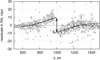Fig. 3. Individual epoch positional residuals ${\mathrm{\Delta }}_{\mathrm{e}}^x$ of stars in the calibration files (open circles with sizes increasing with stellar brightness) for a single epoch in the field of dw14, its approximation Eq. (6) (solid lines) with gx, e = 19.5 mpx, and the astrometric model response WCAL(y) to the step signal gU(y) in the RA positions of stars in chip 2 (dashed lines).

where ${\stackrel{\sim }{\mathit{y}}}_i=|{\mathit{y}}_i-1000|/(0.35R_{\mathrm{opt}})$ is the normalized distance from the chip gap, and a positive (negative) sign is used for stars in chip 2 (chip 1). The fit function (6) shown in Fig. 3 by solid lines nearly coincides with the response function W_CAL(y) (dashed) reproduced from Fig. 1 and normalized to the offset amplitude g = 19.5 ± 0.6 mpx in the measured positional residuals. The estimates of g_x, e in x and g_y, e in y were derived for each epoch e = 1…N_e by a least-squares fit of function (6) to the residuals ${\mathrm{\Delta }}_{i,\mathrm{e}}^x$, ${\mathrm{\Delta }}_{i,\mathrm{e}}^{\mathit{y}}$. The average uncertainty in the determination of the offset g is σ_g = 1.3 mpx.

The change in g_x, e values with time for all sky fields is shown in Fig. 4. The behavior is different for short- (one to one and a half years), medium- (three years), and long-duration (seven years) datasets, which is expected: the astrometric reduction uses the model Eq. (1), which fits the measurements of every star i by the linear change in time caused by proper motion, hence the residuals ${\mathrm{\Delta }}_{i,\mathrm{e}}^x$ and ${\mathrm{\Delta }}_{i,\mathrm{e}}^{\mathit{y}}$ do not change linearly in time. The set of values g for each star field derived later by the least-squares fit Eq. (6) of these residuals are linear combinations of these residuals. Therefore, a set of g_e values for a given star field with its observation time-span also has zero linear dependence on time within the corresponding time intervals, as seen in Fig. 4. In particular, this explains why the g values for short-duration datasets show no trend in 2010–2012, while that is not the case for the longer-duration datasets.

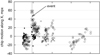Fig. 4. Change in time of chip offset gx, e for sky fields with short (filled dots, six sky fields), medium (crosses, seven fields), and long (open circles, seven fields) observation time-span. The vertical line marks the time of an event that caused a 20–50 mpx offset in gx, e for four fields observed on 20–24 November 2011 (squares).

The vertical line in Fig. 4 marks the time of a large fluctuation on 20–24 November 2011 in four fields. This event is even more prominent in the reduced residuals (Fig. 7).

The discontinuity of W_CAL(y) type is seen in all ξ parameters, for instance, in the parallaxes (cf. Paper I, Fig. 6). Figure 5 shows the distribution of the CAL dataset proper motions for the example case of dw14, which is well approximated by the W_CAL(y) function with an offset amplitude of Δμ = −56.0 ± 5.0 mpx yr⁻¹. The offset terms g and Δμ can be caused by the RCM, but the nonzero offset values for the other parameters ξ are unphysical; they represent the formal fit solution of a model with correlated parameters.

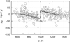Fig. 5. Same as Fig. 3, but for proper motions: the approximation of Eq. (6) (solid lines) and the model response WCAL(y) to the step change Δμ = −56.0 mpx yr−1 in the proper motions of stars in chip 2 (dashed lines).

5. Chip motion retrieved from the calibration files

The definition in Eq. (5) means that the parameter g incorporates information on the epoch residuals of all stars near the chip gap. It is therefore convenient to represent the full star sample for a particular sky field z by one single “equivalent” star that is located right at the chip gap on chip 2 and that has the epoch residuals g_x, z, e, g_y, z, e. For this star, the equivalent proper motions Δμ_x, z, Δμ_y, z were derived by fitting individual stellar motions μ_x, z, i, μ_y, z, i with the function W_CAL(y). The equivalent star displacement at epoch e relative to time t = 0 is

$$\begin{array}{c}\hfill V_{z,\mathrm{e}}^x=g_{x,z,\mathrm{e}}+\mathrm{\Delta }{\mu }_{x,z}{t}_{\mathrm{e}},V_{z,i,\mathrm{e}}^y=g_{y,z,\mathrm{e}}+\mathrm{\Delta }{\mu }_{y,z}{t}_{\mathrm{e}}.\end{array}$$(7)

The values of V can be considered as the measurements in the right side of the model Eq. (4), therefore we rewrite this model into a system of N_e × N_dw × 2 equations,

$$\begin{array}{c}\hfill \begin{array}{c}{\sum }_s{\widehat{\xi }}_{z,s}{\nu }_{s,\mathrm{e}}^x+H^x(t_{\mathrm{e}})+\delta H_{z,\mathrm{e}}^x=V_{z,\mathrm{e}}^x,\hfill \\ {\sum }_s{\widehat{\xi }}_{z,s}{\nu }_{s,\mathrm{e}}^y+H^y(t_{\mathrm{e}})+\delta H_{z,\mathrm{e}}^y=V_{z,\mathrm{e}}^y,\hfill \end{array}\end{array}$$(8)

where z = 1…N_dw is the sky field index, ${\widehat{\xi }}_{z,s}$ are the formal fit parameters (offsets ${\widehat{x}}_z$, ${\widehat{\mathit{y}}}_z$, proper motion ${\widehat{\mu }}_{x,z}$, ${\widehat{\mu }}_{\mathit{y},z}$, etc.), H(t_e) is the smooth component of the RCM, and δH_z, e are the residuals of the fit, which include the measurement errors and the irregular component of the RCM. The fit parameters ${\widehat{\xi }}_{z,s}$ are the corrections to the ξ values in Eq. (1) derived from the primary astrometric solution with H(t) = 0. The system of Eq. (8) allows us to extract H(t). When applied to a single sky field, Eq. (8) returns the trivial solution ${\widehat{\mu }}_z=\mathrm{\Delta }{\mu }_z$, δH_z, e = g_z, e, and H(t_e) = 0. A meaningful solution is found by applying it to all fields. For the function H(t) we adopted the low-order polynomial approximation

$$\begin{array}{c}\hfill H(t)={\displaystyle \sum _{j=0}^n}{h}_j{t}^j\end{array}$$(9)

with n = 3 and n = 1 for the measurements along X and Y, respectively. To separate the fully correlated proper motion and h₁ terms, we required that the sum of proper motions taken over all stars and fields is zero, that is, $\sum _z{\widehat{\mu }}_{x,z}=\sum _z{\widehat{\mu }}_{\mathit{y},z}=0$. With a similar restriction on the stellar position offsets ${\widehat{x}}_z$ and ${\widehat{\mathit{y}}}_z$, we separated these terms and h₀. Thus, the systematic position change in time is fully included in the function H(t), whereas the parameters ${\widehat{x}}_z$, ${\widehat{\mathit{y}}}_z$, ${\widehat{\mu }}_{x,z}$, and ${\widehat{\mu }}_{\mathit{y},z}$ have an average value of zero.

Figure 6 shows the unreduced displacements g_x, z, e + Δμ_x, zt_e, which reveals significant changes of the position of chip 2 relative to chip 1, which reaches offset of 0.2–0.3 pixels in 2016–2018. These displacements are measured consistently in several fields and can therefore not be caused by particular stellar motions. The solution H(t) for the motion along the X-axis is derived from Eq. (8) as a cubic function of time (solid line in Fig. 6). It has an approximately linear segment between 2012 and 2017 where the rate is ∼50 mpx yr⁻¹. Along the Y-axis, the motion is approximately linear at a rate of ∼10 mpx yr⁻¹.

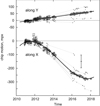Fig. 6. Motion of chip 2 along the X-axis (lower panel) relative to a reference frame defined by stars in both chips: the unreduced displacements $V_{z,\text{e}}^x$ for each epoch e and each sky field z are shown by dots with the typical uncertainty in 2017 (error bar). Solid lines connect the long-duration datasets. The model function H(t) for the motion of chip 2 (thick solid line) and the instant chip motion $H^x(t_{\mathrm{e}})+\delta H_{z,\mathrm{e}}^x$ derived with Eq. (8) (gray circles) are shown as well. The large offset in four fields during 20–24 November 2011 is marked by squares. Upper panel: same for the measurements along the Y-axis.

Figure 7 presents the change in time of the fit residuals δH_z, e for short-, medium-, and long-duration datasets. The residual distribution is approximately random with an rms of 4.3 and 3.8 mpx along the X- and Y-axes, respectively. Weak correlations and departures from the cubic model Eq. (9) can be seen, for example, close to 2017.0. In general, we did not find any strong deviations on timescales of 1–4 days, which means that the RCM is quite smooth in time.

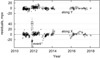Fig. 7. Fit residuals δH between the measured and the position of chip 2 according to the model Eq. (8) relative to chip 1 for each epoch and the sky fields with a short (filled dots), medium (crosses), and long (open circles) duration of observations. An impulse jump for four fields obtained on 20–24 November 2011 is marked by squares.

The only strong variation on timescales of days is found for four fields observed on 20, 22, and 24 November 2011. The large 20–50 mpx offsets occurred within one day because two fields had been observed on November 19 with normal results. This event was probably caused by an intervention on the instrument as part of regular maintenance. Upon our enquiry, the ESO User Support Department confirmed that the FORS2 CCDs were switched on 28 November 2011 and that the observatory records do not indicate an earthquake recovery procedure or FORS2 cryostat warm-up or cool-down cycle on 20–24 November 2011, but that the exact dates of such interventions can sometimes be uncertain.

6. Alternative measurements of the chip motion

In the past section we retrieved the best precise displacement history of RCM using extensive data collected in the calibration files (the CAL dataset derived from multiple reference frames covering all FoVs), and with a reference frame ω set by stars in both chips. In order to confirm this primary result, we investigated the RCM by making several modifications to our astrometric solution. Instead of CAL files, we now used the files of RF datasets (stars of a single reference frame ω per each sky field) and additionally restricted ω space to chip 1. The motion of chip 2 stars then evidently reproduces the RCM effect. However, we found that a robust astrometric solution requires use of the normalizing parameter space ω^* expanded on both chips, in a field within R_opt distance from the dwarf. We also had to update the system of the normalizing conditions Eq. (3) by a model Eq. (10) with a flag λ that allows for two options of the normalization (for details, see Sect. 6.1.1).

Our computations confirm that the RCM does not depend significantly on the choice of the reference frame. Table 2 summarizes the results of determining the RCM with these alternative approaches.

6.1. Motion of chip 2 derived in the reference frame of chip 1

To measure the displacements of chip 2, we performed the astrometric reduction Eqs. (1)–(4) with the reference space ω limited to chip 1 by excluding its segment ω₂ located on chip 2. We first also excluded ω₂ from ω^* (Sect. 6.1.1), and we revised this option in Sect. 6.1.2.

6.1.1. Systematic difference of proper motions between chips

The dependence of the solution coefficients ξ on y, which we illustrate in Fig. 8 for proper motions, is very different from the response function W(y) shown in Fig. 5. The amplitude of the discontinuity Δμ_x, however, is close to that derived with the calibration files.

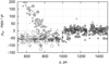Fig. 8. Proper motions μx in the dw14 field derived relative to chip 1 (gray filled circles) and when the astrometric parameters are derived with Eq. (10) (open circles), which allows for a step change between the chips of Δμx = −56.0 mpx yr−1. The circle size is proportional to the stellar brightness.

For stars in chip 2 (y <  1000 px), Fig. 8 shows a clear trend of μ_x, which is natural because the restrictions Eq. (4) do not apply to stars in chip 2 in this case. A flat dependence of ξ on chip 2 is obtained by expanding ω^* over this chip (i.e., by including ω₂ in ω^*) and allowing for a Δξ_s step change in the model Eq. (3):

$$\begin{array}{c}\hfill \begin{array}{c}{{\displaystyle \sum }}_{i\in {\omega }^{\ast }}[{\xi }_{i,s}-\lambda U(y_i)\mathrm{\Delta }{\xi }_s]{\overline{P}}_i=0,s=1\dots S,\hfill \\ {{\displaystyle \sum }}_{i\in {\omega }^{\ast }}{\xi }_{i,s}{\overline{P}}_i{f}_{i,w}(x_i,y_i)=0,s=1\dots S,w=2\dots N^{\prime }.\hfill \end{array}\end{array}$$(10)

Here

$$\begin{array}{c}\hfill \mathrm{\Delta }{\xi }_s={\displaystyle \sum _{i\in {\omega }_2}}{\xi }_{i,s}{\overline{P}}_i/{\displaystyle \sum _{i\in {\omega }_2}}{\overline{P}}_i\end{array}$$(11)

is a new parameter that corresponds to the step change of ξ in chip 2. The λ ∈ [0, 1] parameter allows us to switch this addition on and off. This new model includes the offsets (Δ_x, Δ_y, Δμ_x, Δμ_y, Δρ, Δd, Δϖ) of the parameter values between chips and excludes their systematic change across the FoV.

Figure 8 shows that this approach works because the distribution of μ_x along Y is flat, except for the step change of Δμ_x = −56.0 ± 5.0 mpx yr⁻¹, which is very similar to that obtained from the calibration files, and because the proper motions computed with Eq. (10) (open circles) and when the ω^* space is restricted to chip 1 (gray circles) are nearly identical for y >  1000 px.

6.1.2. Motion of individual stars in the lower chip

With a reference frame anchored in chip 1, the space ω^* expanded to both chips, and the restrictions of Eq. (10) with λ = 1, we obtained a well-behaved step change in the parameters ξ (a typical example is shown in Fig. 8 with open circles). With this model, we ran a primary reduction with Eq. (1) and computed the displacements

$$\begin{array}{c}\hfill V_{z,i,\mathrm{e}}^x={\mathrm{\Delta }}_{z,i,\mathrm{e}}^x+{\mu }_{x,z,i}{t}_{\mathrm{e}},V_{z,i,\mathrm{e}}^y={\mathrm{\Delta }}_{z,i,\mathrm{e}}^y+{\mu }_{y,z,i}{t}_{\mathrm{e}}\end{array}$$(12)

from the initial position of each star. Here Δ_z, i, e are the positional residuals, and μ_z, i are the proper motions of the stars i in the field z. The displacements V_z, i, e do not show any systematic trending in time for stars in the upper chip, but reveal a clear trend in the lower chip, especially in $V_{z,i,\mathrm{e}}^x$. Figure 9 shows the displacements $V_{z,i,\mathrm{e}}^x$ for 15 bright but not saturated stars in each field within a narrow 750 <  y <  1000 px area close to the chip edge. We defined homogeneous star samples and discarded stars with proper motions μ_x, μ_y that deviated strongly from the average Δμ_x, Δμ_y values in a given field.

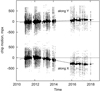Fig. 9. Motion of chip 2 relative to the reference frame of the upper chip: unreduced displacements Vz, i, e along the X- and Y-axes of 15 bright lower chip stars in each sky field at each epoch (small dots). The same after correction for the residual parameters $\widehat{\xi }$ (filled dots). The model motion H(t) (dashed line), which at this scale looks the same for both the unreduced and the corrected displacements.

The sample of data points V_z, i, e presented here directly describes the motion of stars in chip 2 relative to the reference frame anchored in chip 1. Because the displacements are synchronous in all fields, we attribute this effect to the real RCM rather than to peculiar motions of stars. We directly fit the full sample of individual stellar displacements $V_{z,i,\text{e}}^x$ along the X-axis with a cubic function of time and obtained a function (dashed line in Fig. 9) that is similar in shape to the previous estimate of H(t) in Fig. 6.

The values of V_z, i, e vary as a result of the intrinsic proper motions of individual stars, and therefore Fig. 9 appears noisy. To obtain clearer results, we had to mitigate the impact of proper motions. For this purpose we applied Eq. (8) as a secondary reduction model and replaced the right-hand side of the equations by $V_{z,i,\mathrm{e}}^x$ and $V_{z,i,\mathrm{e}}^{\mathit{y}}$ from Eq. (12). This created a system of 15 × N_e × N_dw × 2 equations with polynomial order n = 3 in H^x(t) and n = 1 in H^y(t). We solved it under the s = 1…7 restrictions of ∑_z, iξ_z, i, s = 0. The obtained epoch displacements $H^x(t_{\mathrm{e}})+\delta H_{z,i,\mathrm{e}}^x=V_{z,i,\mathrm{e}}^x-\sum _s{\widehat{\xi }}_{z,i,s}{\nu }_{s,\mathrm{e}}^x$ shown by the solid dots in Fig. 9 differ from the raw displacements $V_{z,i,\mathrm{e}}^x$ only by the single term $\sum _s{\widehat{\xi }}_{z,i,s}{\nu }_{s,\mathrm{e}}$. These new estimates are tightly correlated with the direct approximation of $V_{z,i,\mathrm{e}}^x$, $V_{z,i,\mathrm{e}}^{\mathit{y}}$ obtained from 15 bright stars (dashed lines in Fig. 9). The scatter decreased from the initial ±200 mpx in V_z, e values to ∼20 mpx in the residuals δH_i, e, mainly because we subtracted individual stellar proper motions from the residuals. We found that the RCM is common for all sky fields, as expected, and that deviations from the smooth change in time are smaller than ∼20 mpx.

6.1.3. Chip motion based on the properties of the stellar group

To improve upon the results when 15 stars were used in the previous Section, we formed an equivalent star for each sky field z in the way described in Sect. 5. This artificial star was positioned at the edge of chip 2, represents an ensemble of stars, and is characterized by the displacements

$$\begin{array}{c}\hfill V_{z,\mathrm{e}}^x={\mathrm{\Delta }}_{z,\mathrm{e}}^x+\mathrm{\Delta }{\mu }_{x,z}{t}_{\mathrm{e}},V_{z,\mathrm{e}}^y={\mathrm{\Delta }}_{z,\mathrm{e}}^y+\mathrm{\Delta }{\mu }_{y,z}{t}_{\mathrm{e}}\end{array}$$(13)

measured relative to the reference frame of chip 1. Here, Δ_z, e are the positional residuals, and Δμ_z are the proper motions of the equivalent star in a field z. In Sect. 5, similar estimates were derived from the fit of individual stellar parameters and their variation along Y with the functions W_CAL(y) and G(y). We again used a step function (Fig. 8) fit of individual stars corresponding to the parameter change along Y, derived the estimates at y = 1000 px separately for each chip, and finally obtained Δ_z, e and Δμ_z as the difference between the results in chip 2 and chip 1.

Then, using the model Eq. (8), we derived the residual fit parameters ${\widehat{\xi }}_{z,s}$, the functions H^x(t), H^y(t), and the fit residuals $\delta H_{z,\mathrm{e}}^x$, $\delta H_{z,\mathrm{e}}^{\mathit{y}}$, whose rms of 10 mpx is twice smaller than when individual stars are used (Sect. 6.1.2). The instant displacements H(t)+δH_z, e for each sky field and epoch are shown in Fig. 10 with open circles. The function H^x(t) (solid curve) is close to those obtained in the previous sections with 15 bright stars per field, and to H^x(t) derived using both chips as reference field (Fig. 6). The differences between the estimates of H^y(t) are small considering the uncertainty in proper motions. For both reduction versions the displacement amplitude of chip 2 is ∼0.25 px.

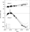Fig. 10. Motion of chip 2 along RA (lower panel) and Dec (upper panel) relative to chip 1. Each curve is the solution for H(t) derived with the models in Table 2, as indicated by the legend. The instant motion estimate H(t)+δHz, e for model 2 (open circles) shows the scatter in the RCM determination for individual fields and epochs. The step change in four fields observed on 20–24 November 2011 and derived with approaches 2 and 4 is marked by squares.

We obtained one more estimate of H(t) with the reference frame anchored in chip 1, where we used the full FoV as a space ω^* for the normalization Eqs. (10) and (11) of parameters ξ, but instead of λ = 1, we set λ = 0 (Nr.3 in Table 2). Now, the parameters ξ follow a change that is approximated by the functions W_CAL(y) or G(y). Using these functions to fit the individual stellar parameters, we formed the equivalent stars for each sky field described by the group parameters Δ_z, e and Δμ_z. A subsequent reduction derived the model motion H(t) that is shown by the dash-dotted curve in Fig. 6 and ∼10 mpx for the rms of fit residuals δH_z, e.

6.2. Using Gaia DR2 to estimate the chip motion

We used the Gaia DR2 catalog (Lindegren et al. 2018; Gaia Collaboration 2018) as an absolute calibrator to convert differential FORS2 astrometry into the ICRF coordinate system (ICRS). In this system, the RCM is apparent as a change in the astrometric zero-points of the CCD chips. To measure this effect, we converted FORS2 into ICRS at every observation epoch. For the seven fields with the longest time-span, we have 147 epoch measurements, thus we obtained 147 estimates of the relative chip position in 2010–2018. The CCD epoch positions

$$\begin{array}{c}\hfill {\overline{x}}_{z,i,\mathrm{e}}=x_{z,i,0}+V_{z,i,\mathrm{e}}^y,{\overline{y}}_{z,i,\mathrm{e}}=y_{z,i,0}+V_{z,i,\mathrm{e}}^y\end{array}$$(14)

converted into ICRS are formed from the ith star position x_z, i, 0, y_z, i, 0 in the reference image (m = 0) and the displacements $V_{z,i,\mathrm{e}}^x$, $V_{z,i,\mathrm{e}}^{\mathit{y}}$ computed with Eq. (12) for each sky field z. Thus, we used Δ_z, e and Δμ_z as previously derived with the astrometric reduction based on the reference frame ω limited to chip 1, and the space ω^* set to all FoVs (Nr. 4 in Table 2).

The zero-point estimates potentially depend on the exact sample of stars used at a given epoch. We mitigated this by using the stars that are common to all epochs. This common star list was derived at the first identification between FORS2 and Gaia at the epoch nearest to the Gaia reference epoch T_DR2 = 2015.5. The identification procedure was similar to that described in Lazorenko & Sahlmann (2017, 2018), where we used full bivariate polynomials of the maximum power n for the transformation between catalogs. We used stars in both chips for this transformation. To take the relative displacement of chip 2 into account, we expanded these transformation functions with two additional free parameters $\mathrm{\Delta }{F}_{\mathrm{e},z}^x$ and $\mathrm{\Delta }{F}_{\mathrm{e},z}^{\mathit{y}}$ that we added to the zero-points of chip 2 only and set to zero for chip 1. This model integrates information on the relative position of the reference frames and thus on the relative motion of chips. Upon the estimation of ΔF_e, z, we find the instant displacements

$$\begin{array}{c}\hfill H_z^x(t_{\mathrm{e}})+\delta H_{z,\mathrm{e}}^x=\mathrm{\Delta }{F}_{\mathrm{e},z}^x-{\overline{\mathrm{\Delta }F}}_z^x{H}_z^y(t_{\mathrm{e}})+\delta H_{z,\mathrm{e}}^y=\mathrm{\Delta }{F}_{\mathrm{e},z}^y-{\overline{\mathrm{\Delta }F}}_z^y,\end{array}$$(15)

where ${\overline{\mathrm{\Delta }F}}_z$ is the average offset in a field z on 2011–2012. We tested all polynomial orders n up to the maximum n = 7, and its best-fit value was found using an F-test for the rejection of insignificant coefficients as described in Lazorenko & Sahlmann (2017). We found that n = 5 fit most fields best.

We set the cross-match radius to 3.3σ₁, where σ₁ is the model uncertainty that includes all known errors of FORS2 and Gaia DR2, and is 1–2 mas for G = 16–19 mag stars at the epochs near T_DR2. In different fields we identified between 43 to 206 stars that FORS2 and DR2 had in common. For the epochs ±0.5 yr within T_DR2 = 2015.5, we obtained the unbiased rms of individual differences between FORS2 and Gaia positions σ_F − G = 1 − 2.5 mas, which is close to the expected value of σ₁. The dominant error component of σ₁ is the uncertainty of Gaia proper motions of about 0.3–1 mas yr⁻¹. For this reason, σ_F − G is minimum on T_DR2 and increases to 4–7 mas at the 2011 and 2017 epochs.

In some fields we found fewer than expected cross-matched stars in chip 2, and the number was too low to determine ΔF_e, z reliably. Better results were obtained when the common star list was created from the identification made at the first epoch of the sky field exposure (2011–2012). For these epochs, which are distant from T_DR2, a higher value of σ₁ and thus a wider identification window favorably increased the common star number. With this approach, the σ_F − G value increased slightly but the uncertainty in the determination of ΔF_e, z improved significantly in some fields. Finally, we obtained the values ΔF_e, z and computed the instant motion of chip 2 H_z(t_e) that we present in Fig. 11 with Eq. (15). These estimates can be approximated by the polynomials

$$\begin{array}{c}\hfill \begin{array}{c}{H}^x(t)=-204.5-76.78t+4.66t^2+2.701t^3\mathrm{mpx},\hfill \\ H^y(t)=46.7+13.31t\mathrm{mpx}\hfill \end{array}\end{array}$$(16)

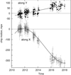Fig. 11. Motion of chip 2 along RA (lower panel) and Dec (upper panel) relative to the upper chip derived using Gaia DR2: instant estimates Hz(te)+δHz, e for individual sky fields z and epochs e (open circles) and the smooth fit functions H(t).

with uncertainties of ±0.08 and ±0.04 mpx for the linear coefficients in RA and Dec, respectively, and t is measured relative to T_DR2. In 2017.5, H^x = −318 mpx and H^y = 67 mpx, which matches the estimates derived with the other approaches (Table 2) relatively well.

7. Calibration of and correction for the chip motion

The relative displacement of the chips directly affects the position of the target by adding a bias to the epoch residuals Δ_z, e (see Fig. 3). According to Eq. (6), the bias value G(y) depends on the amplitude g, the target distance from the division line between chips, and the reference field size R_opt. Typically, g_x = 10 − 20 mpx and R_opt = 500 − 1000 px, which for a target located at y = 1100 px results in an RA bias of ≈3–6 mpx or 0.4–0.7 mas at a single epoch. This is a rough estimate for the rms variation of the bias added to the epoch residuals, which we denote as σ_bias and which is very large in comparison to the FORS2 astrometric uncertainty of ∼0.1 mas. In the extreme events of g ≈ 60 mpx, the bias in these epoch residuals can reach 2 mas. This bias therefore needs to be identified, modeled, and removed.

The bias can be removed in two ways: either using the discrete estimates g_e derived from the calibration files, or using the analytic approximations for H(t) derived in Sects. 6.1 and 6.2. In the first case, incorrectly assuming that the RCM is a random process that is not correlated in time, we expect that H(t_e) = g_e, so that a simple correction x_m − g_x, e, x_m − g_y, e applied to the measurements of stars in chip 2 eliminates the effect.

However, the values of H(t_e) are clearly correlated and reflect the mostly smooth motion of the chips. The models of H(t) derived in Sects. 5 and 6.1 are sums of the linear and nonlinear components H₂₃(t) with quadratic and cubic (t² and t³) terms. The linear component is included in the proper motions of stars and therefore does not affect the computation of the epoch residuals and g values. The following discussion therefore does not concern the RCM along Y, which is linear in time.

The component H₂₃(t) produces RCM variations of ±20 − 50 mpx amplitude and correlated on a 1–2 yr timescale (Fig. 12). The astrometric reduction redistributes the H₂₃(t) variations across the model parameters ξ and the epoch residuals. Moreover, because some sky fields are observed within a restricted time interval Δt, instead of H₂₃(t), we detected only the remnants ${\widehat{H}}_{23}(t)=H(t)-a_{\mathrm{\Delta }t}-b_{\mathrm{\Delta }t}t$ of this function after subtracting the linear fit a_Δt + b_Δtt over the time interval Δt specific to a field. The shape of H₂₃(t) therefore depends on Δt, and the variation amplitude increases with Δt. Thus, H(t) is not fully reflected in the epoch residuals, and we consequently measure a reduced value of g_e.

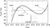Fig. 12. Nonlinear component $H_{23}^x(t)$ of the displacement of chip 2 in time derived with approaches 1–4 listed in Table 2, and their average ⟨H⟩ (thick solid line) for the long-duration datasets (Δt = 7 yr), and $H_{23}^x(t)$ corresponding to ⟨H⟩ for the short-duration (Δt = 1.5 yr) and medium-duration (Δt = 3 yr) datasets.

This is illustrated with Fig. 13, where we compare the measured g_x, z, e values derived from the CAL files for each sky field z and epoch e, and ${\widehat{H}}_{23}(t)$ derived using Gaia DR2 and explicitly set by Eq. (16) for H(t). This graph shows that the g values are on average lower than the expected ${\widehat{H}}_{23}(t)$ values. We find a linear dependence

$$\begin{array}{c}\hfill g_{\mathrm{e}}=K{\widehat{H}}_{23}(t)\end{array}$$(17)

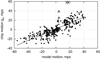Fig. 13. Correlation between the epoch displacements in chip 2, gx, along RA in 20 sky fields derived with the standard reduction (Nr.1 in Table 2) and the nonlinear component of the chip motion ${\widehat{H}}_{23}(t)$ derived with use of Gaia DR2 (Nr.4 in Table 2). The fitted line has a slope of K = 0.63 ± 0.03. The measurements on 20–24 November 2011 are shown by squares and triangles for the medium- and short-duration datasets, respectively.

between these values with a slope of K = 0.63 ± 0.03. Thus, given the measured g_e value, the statistical RCM is ${\widehat{H}}_{23}(t_{\mathrm{e}})=(1/K)g_{\mathrm{e}}=(1/0.63)g_{\mathrm{e}}$, which is close to the empirical (1/0.70)g_e estimate derived in Paper I. Similar estimates for K were obtained with other models of RCM, for instance, 0.62 ± 0.03 and 0.58 ± 0.02 for solutions 2 and 3 of Table 2. With the correction

$$\begin{array}{c}\hfill x_m^{\mathrm{corr}}=x_m-K^{-1}{g}_{x,\mathrm{e}},y_m^{\mathrm{corr}}=y_m-K^{-1}{g}_{y,\mathrm{e}}\end{array}$$(18)

applied to the measurements of stars in chip 2, the systematic change in residuals with Y similar to that shown in Fig. 3 is removed (Paper I, Sect. 4.3.2, Fig. 5). Given the average uncertainty σ_g = 1.3 mpx of the g determination, the effect of RCM in the epoch residuals of targets at y₀ = 1100 px decreases by one order of magnitude from the initial σ_bias = 3–6 mpx to σ_bias = K⁻¹σ_gg⁻¹G(y₀) ≈ 0.6 mpx or ±0.07 mas. This residual bias is acceptable for FORS2 astrometry.

Alternatively, the RCM can be removed directly using one of the derived model functions H(t). As explained above, it is sufficient to apply these corrections for the nonlinear motion components only because the linear component (i.e., the case of Dec) does not affect the epoch residuals. In the previous sections we obtained a few estimates of H(t) whose nonlinear components H₂₃(t_e) (Fig. 12) are slightly dispersed, and we formed their average ⟨H⟩ to obtain more reliable results. The rms of the individual H₂₃(t_e) relative to ⟨H⟩ is 6.1 mpx, therefore the formal uncertainty of ⟨H⟩ is σ′≈3.1 mpx. We can now correct for RCM by applying the correction

$$\begin{array}{c}\hfill x_m^{\mathrm{corr}}=x_m-⟨H(t_{\mathrm{e}})⟩\end{array}$$(19)

to stars in chip 2. For stars at y₀ = 1100 px, the bias is expected to decrease to σ_bias = σ′g⁻¹G(y₀) ≈ ± 0.12 mas, which is larger than the residual bias obtained when g_e is used.

We verified the above estimates with the complete astrometric reduction of dw14 by including and excluding the RCM corrections Eqs. (18) and (19). We applied a reduction model based on Eqs. (1) and (3) (or, equivalently, Eq. (10) with λ = 0) using circular ω and ω^* spaces of R_opt = 711 px radius centered at dw14. This is a standard model for astrometric reduction on FORS2 (Sahlmann et al. 2014; Lazorenko et al. 2014), but now we take into consideration that ω and ω^* spaces are fragmented into two sections that are related to different chips.

Without the RCM correction, the astrometric reduction produced the epoch residuals ${\mathrm{\Delta }}_{\mathrm{e}}^x$ shown in Fig. 14 by gray circles for the example epoch on 17 February 2012, which can be compared to Fig. 3 at the same epoch, but based on the calibration files (Sect. 3.2). The plots are similar in shape, but the distribution of ${\mathrm{\Delta }}_{\mathrm{e}}^x$ in Fig. 14 is now not exactly symmetric relative to y = 1000 px because the reference field center is 73 px off this line. Moreover, the number of stars is twice smaller than in the calibration files because of the limited R_opt size.

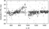Fig. 14. Epoch residuals ${\mathrm{\Delta }}_{\mathrm{e}}^x$ for reference stars in the field of dw14 obtained in a single epoch (same as in Fig. 3) without correction for RCM (gray circles) and after correction with Eq. (18) and K = 0.63 (open circles).

The systematic value of ${\mathrm{\Delta }}_{\mathrm{e}}^x$ at some y is the bias in the position of the object located there, so that for dw14 at y = 1073 px the bias in the example epoch is roughly 0.28g_x, e≈5 mpx or 0.6 mas. The rms value ${\widehat{\sigma }}_{\mathrm{bias}}$ of the bias taken over all epochs is 0.55 mas. This includes the uncertainty of the fit σ_fit = 0.06 mas, which we subtracted quadratically and obtained σ_bias = 0.54 mas. This value characterizes the bias in the epoch residuals without correction of RCM (Table 3).

The efficiency of the correction with Eq. (18) is evident from Fig. 14, which displays the new residuals ${\mathrm{\Delta }}_{\mathrm{e}}^x$ (open circles) computed with the positions $x_m^{\mathrm{corr}}$, ${\mathit{y}}_m^{\mathrm{corr}}$ of stars in chip 2 corrected for each image m. The distribution of ${\mathrm{\Delta }}_{\mathrm{e}}^x$ along Y is now flat. For the example epoch and objects at y = 1073 px, this calibration decreases the bias to 0.3 mpx. For all epochs, the average rms bias for the target is ${\widehat{\sigma }}_{\mathrm{bias}}=0.06$–0.07 mas; it is equally good for the two tested coefficient values of K = 0.70 and K = 0.63. By quadratically subtracting σ_fit, we find σ_bias = 0.02 mas for the correction with K = 0.63.

This is the best way of removing the RCM effect and reducing its impact to the noise level. We also find that for the epoch shown in Fig. 14 this calibration decreased the rms of Δ_e for bright 17–18 mag stars from 4.2 mpx (=0.5 mas) to 1.0 mpx (=0.12 mas), which is a typical uncertainty of the epoch residuals for FORS2 astrometry.

A significant but insufficient decrease of σ_bias to 0.16 mas (Table 3) was also obtained with the calibration of Eq. (19). This result indirectly suggests that the true RCM follows a smooth cubic polynomial change in time, but that the updated model of H(t) should include higher order terms in t and possibly some irregular displacements like those that took place on 20–24 November 2011. For comparison, we repeated these computations for the ultracool dwarfs 3 and 11 listed in Table 1 by Sahlmann et al. (2014), which represent short- and medium-duration datasets, respectively.

Summarizing these results, we conclude that the RCM effect is comparable for long- and medium-duration datasets and can be removed well using g values based on calibration files. For short-duration datasets, the RCM adds a small bias that does not significantly degrade the astrometric precision even when left uncorrected.

8. Conclusion

Astrometric programs often require a reference field whose size exceeds a single chip. For multi-chip detectors it is therefore natural to use stars both in the primary chip where the target object is imaged and in the adjacent chips. In the case of FORS2, the reference field partially covers the primary chip 1, but for precise astrometric reduction it is often extended to the second chip 2. The use of such multi-chip reference frames implies that the locations of the chips within a detector are known.

First signs of internal chip motions within the FORS2 detector were reported in Paper I. Here, we investigated this effect in detail using images of sky fields that were monitored over a few years (Sahlmann et al. 2014). We used several approaches: the motion of chip 2 was measured relative to chip 1 or relative to the reference frame extended over both chips, and we used the Gaia DR2 catalog. All approaches yielded concordant results in which the motion of chip 2 varied in time with an amplitude of up to ∼70 mpx yr⁻¹. The full amplitude of the chip displacement between 2011 and 2018 is 0.3 px or 38 mas in the direction along the line that divides the chips. In the orthogonal direction (i.e., across the chip gap) the displacements is ∼0.07 px.

The dominant relative chip motion follows a cubic dependence on time in RA and changes its direction in 2011.8 from positive to negative, and it seems to invert again in 2017.5. In addition, we found significant deviations from a smooth continuous motion. For example, we detected a step-like displacement by 0.02–0.05 px (2–6 mas) that occurred on 20–24 Nov. 2011 and was likely caused by an instrument maintenance intervention. In the orthogonal direction, the relative chip motion appears linear in time.

On average, the relative chip motion adds a random component to the epoch residuals of ∼0.5 mas, thus it can significantly degrade the FORS2 astrometric performance of 0.1 mas for a single epoch if it is not corrected for. We demonstrated that the relative chip motion effect can be mitigated to the noise level at the cost of extensive computations that are needed to create special calibration files.

The relative chip motion was investigated by Bernstein et al. (2017), who analyzed the stability of a 61 CCD chip array of the Dark Energy Camera (DECam; Flaugher et al. 2015) and discovered displacements of chips with an amplitude of 0.4 px = 100 mas, or 6 μm. Although these estimates are comparable to those we obtained for FORS2, they refer to the detectors of a quite different design and linear dimensions. The DECam CCDs cover a very large ∼450 × 450 mm space, so that the displacement values are 10⁻⁵ relative to the detector size only, while we found ∼10⁻⁴ for FORS2. The motions of the DECam CCDs were found to be closely related to the warming or cooling thermal recycling, which appears as a stochastic change in time. In contrast, the motion of FORS2 chips within the MIT detector is smooth and linear in time, at least between 2012 and 2018, and does not depend much on the thermal recycling during the exchanges between the MIT and E2V mosaic detectors, which occur with a spacing of a few months. For these reasons, we consider that the relative chip motion in the case of FORS2 is of a different physical nature and potentially reflects some aging processes.

We demonstrated that chip array instabilities can seriously degrade high-precision astrometry if left uncorrected. The MICADO near-infrared camera (Davies et al. 2010) for the ELT aims at a single-epoch accuracy of ≤50 μas over an FOV of 53″ (Rodeghiero et al. 2018; Pott et al. 2018). The detector of MICADO is a 3  ×  3 array, and if the reference field is expanded over the full FoV, the RCM effect can fragment it into 3  ×  3 segments. In the hypothetical case that the relative chip motion of MICADO is comparable to FORS2, it can introduce biases of 50–300 μas in the target epoch positions if the reference field extends over several chips and the effect is not calibrated and corrected using dedicated methods (e.g., Rodeghiero et al. 2019).

Our findings underline that chip stability needs to be considered. Dedicated monitors for detector arrays may need to be implemented that are expected to fulfill the stringent requirements of astrometric performances.

References

All Tables

All Figures

Fig. 1. Simulation of the astrometric model response to a step change U(y) in the position of chip 2 for the example sky field of dw14 offset by 73 px from the detector center. Dots show the response in the epoch residuals ${\mathrm{\Delta }}_{i,\mathrm{e}}^x$ of reference stars, and the function WRF is the smoothed response in proper motions to the step change of proper motions of chip 2 stars. The function WCAL is the same, but for the reference stars distributed evenly over FoV.

In the text

	Fig. 2. Epoch positional residuals ${\mathrm{\Delta }}_{\mathrm{e}}^x$ for bright reference stars imaged close to the chip gap in the sky field of dw14. The residuals are shown separately for stars in chip1 and chip 2 and exhibit an anticorrelated pattern.
In the text

Fig. 3. Individual epoch positional residuals ${\mathrm{\Delta }}_{\mathrm{e}}^x$ of stars in the calibration files (open circles with sizes increasing with stellar brightness) for a single epoch in the field of dw14, its approximation Eq. (6) (solid lines) with gx, e = 19.5 mpx, and the astrometric model response WCAL(y) to the step signal gU(y) in the RA positions of stars in chip 2 (dashed lines).

In the text

	Fig. 4. Change in time of chip offset gx, e for sky fields with short (filled dots, six sky fields), medium (crosses, seven fields), and long (open circles, seven fields) observation time-span. The vertical line marks the time of an event that caused a 20–50 mpx offset in gx, e for four fields observed on 20–24 November 2011 (squares).
In the text

	Fig. 5. Same as Fig. 3, but for proper motions: the approximation of Eq. (6) (solid lines) and the model response WCAL(y) to the step change Δμ = −56.0 mpx yr−1 in the proper motions of stars in chip 2 (dashed lines).
In the text

Fig. 6. Motion of chip 2 along the X-axis (lower panel) relative to a reference frame defined by stars in both chips: the unreduced displacements $V_{z,\text{e}}^x$ for each epoch e and each sky field z are shown by dots with the typical uncertainty in 2017 (error bar). Solid lines connect the long-duration datasets. The model function H(t) for the motion of chip 2 (thick solid line) and the instant chip motion $H^x(t_{\mathrm{e}})+\delta H_{z,\mathrm{e}}^x$ derived with Eq. (8) (gray circles) are shown as well. The large offset in four fields during 20–24 November 2011 is marked by squares. Upper panel: same for the measurements along the Y-axis.

In the text

	Fig. 7. Fit residuals δH between the measured and the position of chip 2 according to the model Eq. (8) relative to chip 1 for each epoch and the sky fields with a short (filled dots), medium (crosses), and long (open circles) duration of observations. An impulse jump for four fields obtained on 20–24 November 2011 is marked by squares.
In the text

	Fig. 8. Proper motions μx in the dw14 field derived relative to chip 1 (gray filled circles) and when the astrometric parameters are derived with Eq. (10) (open circles), which allows for a step change between the chips of Δμx = −56.0 mpx yr−1. The circle size is proportional to the stellar brightness.
In the text

Fig. 9. Motion of chip 2 relative to the reference frame of the upper chip: unreduced displacements Vz, i, e along the X- and Y-axes of 15 bright lower chip stars in each sky field at each epoch (small dots). The same after correction for the residual parameters $\widehat{\xi }$ (filled dots). The model motion H(t) (dashed line), which at this scale looks the same for both the unreduced and the corrected displacements.

In the text

Fig. 10. Motion of chip 2 along RA (lower panel) and Dec (upper panel) relative to chip 1. Each curve is the solution for H(t) derived with the models in Table 2, as indicated by the legend. The instant motion estimate H(t)+δHz, e for model 2 (open circles) shows the scatter in the RCM determination for individual fields and epochs. The step change in four fields observed on 20–24 November 2011 and derived with approaches 2 and 4 is marked by squares.

In the text

	Fig. 11. Motion of chip 2 along RA (lower panel) and Dec (upper panel) relative to the upper chip derived using Gaia DR2: instant estimates Hz(te)+δHz, e for individual sky fields z and epochs e (open circles) and the smooth fit functions H(t).
In the text

	Fig. 12. Nonlinear component $H_{23}^x(t)$ of the displacement of chip 2 in time derived with approaches 1–4 listed in Table 2, and their average ⟨H⟩ (thick solid line) for the long-duration datasets (Δt = 7 yr), and $H_{23}^x(t)$ corresponding to ⟨H⟩ for the short-duration (Δt = 1.5 yr) and medium-duration (Δt = 3 yr) datasets.
In the text

Fig. 13. Correlation between the epoch displacements in chip 2, gx, along RA in 20 sky fields derived with the standard reduction (Nr.1 in Table 2) and the nonlinear component of the chip motion ${\widehat{H}}_{23}(t)$ derived with use of Gaia DR2 (Nr.4 in Table 2). The fitted line has a slope of K = 0.63 ± 0.03. The measurements on 20–24 November 2011 are shown by squares and triangles for the medium- and short-duration datasets, respectively.

In the text

	Fig. 14. Epoch residuals ${\mathrm{\Delta }}_{\mathrm{e}}^x$ for reference stars in the field of dw14 obtained in a single epoch (same as in Fig. 3) without correction for RCM (gray circles) and after correction with Eq. (18) and K = 0.63 (open circles).
In the text

References

- Anderson, J., & King, I. R. 2003, PASP, 115, 113 [NASA ADS] [CrossRef] [Google Scholar]
- Appenzeller, I., Fricke, K., Fürtig, W., et al. 1998, The Messenger, 94, 1 [NASA ADS] [Google Scholar]
- Bernstein, G. M., Armstrong, R., Plazas, A. A., et al. 2017, PASP, 129, 074503 [NASA ADS] [CrossRef] [Google Scholar]
- Davies, R., Ageorges, N., & Barl, L. 2010, in Ground-based and Airborne Instrumentation for Astronomy III, Proc. SPIE, 7735, 77352A [NASA ADS] [Google Scholar]
- Flaugher, B., Diehl, H. T., Honscheid, K., et al. 2015, AJ, 150, 150 [NASA ADS] [CrossRef] [Google Scholar]
- Gaia Collaboration 2018, VizieR Online Data Catalog: I/345 [Google Scholar]
- Garcia, E. V., Ammons, S. M., Salama, M., et al. 2017, ApJ, 846, 97 [NASA ADS] [CrossRef] [Google Scholar]
- Lazorenko, P. F., & Lazorenko, G. A. 2004, A&A, 427, 1127 [NASA ADS] [CrossRef] [EDP Sciences] [Google Scholar]
- Lazorenko, P. F., & Sahlmann, J. 2017, A&A, 606, A90 [NASA ADS] [CrossRef] [EDP Sciences] [Google Scholar]
- Lazorenko, P. F., & Sahlmann, J. 2018, A&A, 618, A111 [NASA ADS] [CrossRef] [EDP Sciences] [Google Scholar]
- Lazorenko, P. F., Mayor, M., Dominik, M., et al. 2009, A&A, 505, 903 [NASA ADS] [CrossRef] [EDP Sciences] [Google Scholar]
- Lazorenko, P. F., Sahlmann, J., Ségransan, D., et al. 2014, A&A, 565, A21 [NASA ADS] [CrossRef] [EDP Sciences] [Google Scholar]
- Lindegren, L., Hernández, J., Bombrun, A., et al. 2018, A&A, 616, A2 [NASA ADS] [CrossRef] [EDP Sciences] [Google Scholar]
- Pott, J. U., Rodeghiero, G., & Riechert, H. 2018, in Ground-based and Airborne Instrumentation for Astronomy VII, SPIE Conf. Ser., 10702, 1070290 [Google Scholar]
- Rodeghiero, G., Pott, J.-U., Arcidiacono, C., et al. 2018, MNRAS, 479, 1974 [NASA ADS] [CrossRef] [Google Scholar]
- Rodeghiero, G., Sawczuck, M., Pott, J.-U., et al. 2019, PASP, 131, 054503 [NASA ADS] [CrossRef] [Google Scholar]
- Sahlmann, J., Lazorenko, P. F., Ségransan, D., et al. 2014, A&A, 565, A20 [NASA ADS] [CrossRef] [EDP Sciences] [Google Scholar]
- Sahlmann, J., Burgasser, A. J., Martín, E. L., et al. 2015a, A&A, 579, A61 [NASA ADS] [CrossRef] [EDP Sciences] [Google Scholar]
- Sahlmann, J., Lazorenko, P. F., Ségransan, D., et al. 2015b, A&A, 577, A15 [NASA ADS] [CrossRef] [EDP Sciences] [Google Scholar]
All Tables
Summary of the spaces ω, ω*, and flags λ that specifies different modifications of astrometric reduction, and the estimated displacement of chip 2 along the X-axis from 2012.0 to 2017.5.
rms of additional bias σbias in the epoch residuals in mas obtained with and without RCM correction, for the short-, medium-, and long-duration datasets indicated by Δt.