| Issue |
A&A
Volume 629, September 2019
|
|
|---|---|---|
| Article Number | A3 | |
| Number of page(s) | 20 | |
| Section | Catalogs and data | |
| DOI | https://doi.org/10.1051/0004-6361/201936074 | |
| Published online | 22 August 2019 | |
The HST Key Project galaxies NGC 1326A, NGC 1425, and NGC 4548: New variable stars and massive star population⋆
1
IAASARS, National Observatory of Athens, 15236 Penteli, Greece
e-mail: This email address is being protected from spambots. You need JavaScript enabled to view it.
2
Department of Astrophysics, Astronomy & Mechanics, Faculty of Physics, University of Athens, 15783 Athens, Greece
3
Astronomický ústav, Akademie věd České republiky, Fričova 298, 251 65 Ondřejov, Czech Republic
Received:
12
June
2019
Accepted:
11
July
2019
Abstract
Studies of the massive star population in galaxies beyond the Local Group are the key to understanding the link between their numbers and modes of star formation in different environments. We present the analysis of the massive star population of the galaxies NGC 1326A, NGC 1425, and NGC 4548 using archival images obtained with the Hubble Space Telescope Wide Field Planetary Camera 2 in the F555W and F814W filters. Through high-precision point spread function fitting photometry for all sources in the three fields, we identified 7640 candidate blue supergiants, 2314 candidate yellow supergiants, and 4270 candidate red supergiants. We provide an estimate of the ratio of blue to red supergiants for each field as a function of galactocentric radius. Using Modules for Experiments in Stellar Astrophysics (MESA) at solar metallicity, we defined the luminosity function and estimated the star formation history of each galaxy. We carried out a variability search in the V and I filters using three variability indexes: the median absolute deviation, the interquartile range, and the inverse von Neumann ratio. This analysis yielded 243 new variable candidates with absolute magnitudes ranging from MV = −4 to −10 mag. We classified the variable stars based on their absolute magnitude and their position on the color–magnitude diagram using the MESA evolutionary tracks at solar metallicity. Our analysis yielded 8 candidate variable blue supergiants, 12 candidate variable yellow supergiants, 21 candidate variable red supergiants, and 4 candidate periodic variables.
Key words: galaxies: individual: NGC 1326A / galaxies: individual: NGC 1425 / galaxies: individual: NGC 4548 / stars: massive / supergiants / stars: variables: general
Full Tables 1, 2, 3, and Tables 6–10 are only available at the CDS via anonymous ftp to cdsarc.u-strasbg.fr (130.79.128.5) or via http://cdsarc.u-strasbg.fr/viz-bin/qcat?J/A+A/629/A3
© ESO 2019
1. Introduction
Variability studies at large distances can be used as a powerful tool to study the pre-supernova state and evolved states of massive stars (Kochanek et al. 2017). The open questions of stellar evolution regarding mass loss, internal mixing, and stellar winds (Langer 2012; Massey 2003) have frequently been investigated in conjunction with photometric variability studies (Bonanos 2007; Yang & Jiang 2012; Kourniotis et al. 2017; Soraisam et al. 2018). The evolution of very massive stars is quite uncertain both due to the limited observational samples and physical processes that trigger variability. For example, the origin of variability in the light curves of luminous blue variables (LBVs) in metal-poor environments (Kalari et al. 2018), the physical mechanisms causing shear-induced instabilities in massive stars (Maeder & Meynet 2000; Heger & Langer 2000), or evolutionary paths leading to binarity in yellow and red supergiants (Prieto et al. 2008; Moriya 2018) are some of the open questions that are yet to be investigated. The short evolution timescale combined with the rarity of massive stars is the greatest challenge in testing stellar evolutionary models against observations. A solution to overcome the problem of the limited observational sample of massive stars is to take advantage of the large amount of existing archival data.
Archival data from the Hubble Space Telescope (HST) allow us to extend the studies of massive stars and trace star formation beyond the Local Group. Archives are widely recognized as a valuable resource for astronomy. The large sample of deep extragalactic HST observations gives us the opportunity to study in detail the stellar population of blue supergiants (BSGs), yellow supergiants (YSGs), and red supergiants (RSGs) in galaxies beyond 10 Mpc. Studying massive stars at larger distances is the key to understanding whether the evolution of massive stars is different in different environments. For example, the ratio of the BSGs to RSGs (B/R) as a function of metallicity and galactocentric radius is one of the diagnostic tools that are applied to study metallicity, star formation, mass loss, and convection processes (Brunish et al. 1986; Langer & Maeder 1995). Our previous study on the massive star population of the Virgo cluster galaxy NGC 4535 (Spetsieri et al. 2018, Paper I) demonstrates the importance of archival HST data for extragalactic studies on massive stars. NGC 4535 was studied by Macri et al. (1999) for Cepheid variables as part of the HST Key project and 50 Cepheid variables were detected. Using data from the HST, we conducted our own photometry for NGC 4535 aiming to identify more massive variable stars. Our study unveiled 120 new variable massive stars, among which are eight luminous candidate RSGs, four candidate YSGs, and one candidate LBV.
In this study we aim to expand our search for massive stars, using the same method as we adopted in Paper I for three other galaxies that were studied in the HST Key project: NGC 1326A (Prosser et al. 1999), NGC 1425 (Mould et al. 2000) and the Virgo cluster galaxy NGC 4548 (Graham et al. 1999). All three fields were previously studied for Cepheid variables; 15 Cepheids are reported in NGC 1326A, 20 in NGC 1425, and 24 in NGC 4548. However, the existence of other objects that were not classified as Cepheids but showed variability in their light curve (Graham et al. 1999) is yet to be investigated. These three galaxies were selected as metal-rich galaxies with high star formation rates (SFRs) that can help to provide a better view of the variability displayed in the massive star population because massive stars serve as the primary source of carbon, nitrogen, and oxygen (CNO) enrichment of the interstellar medium (ISM) and are progenitors of supernovae (Conroy et al. 2018; Maeder et al. 1980).
The paper is structured as follows: the observations and data reduction are presented in Sect. 2, the massive star populations of NGC 1326A, NGC 1425, and NGC 4548 and the B/R are described in Sect. 3. The selection of variable candidates and the classification of the new massive variable candidates is described in Sect. 4. The summary is given in Sect. 5.
2. Observations and reduction
2.1. Observations
We used archival observations of NGC 1326A, NGC 1425, and NGC 4548 taken with the HST WFPC2 as described in Freedman et al. (2001) as part of the HST Key Project. For the three galaxies, we used the observations available in filters F555W (equivalent to the Johnson V filter) and F814W (equivalent to Kron-Cousins I). In particular, we used 13 epochs of observations in F555W and 8 epochs in F814W that are available for the galaxies NGC 1326A and NGC 4548, while for NGC 1425, we used the 14 available epochs in F555W and 8 in F814W. The F555W data consisted of 3 × 1200 s exposures and 4 × 1300 s exposures, and the F814W data consisted of 3 × 1300 s exposures. Data were collected at four dithering positions, with one quarter of the observations (four pairs of F814W images and two pairs of F555W images) taken at each position. We retrieved the pre-reduced images through the Mikulsky Archive for Space Telescopes1 and performed point spread function (PSF) photometry using the latest WFPC2 module of DOLPHOT (updated in 2016), which is a modified version of HSTphot (Dolphin 2000).
2.2. Reduction
We proceeded with the photometric reduction as described in the manual of the WFPC2 module of DOLPHOT and in Paper I. We applied the photometric quality criteria listed in the DOLPHOT manual to distinguish the isolated point-like sources from the extended sources detected by DOLPHOT. The criteria were a signal-to-noise ratio S/N ≥ 10, −0.3≤, sharpness ≤0.3, χ2 ≤ 2.5, and object type=1. The resulting catalog for each field includes the coordinates of each source in RA, Dec (J2000), X, Y, and mean magnitude in V and I filters. The total number of stars after the quality cuts is 5897 stars in NGC 1326A, 5232 stars in NGC 1425, and 5790 stars in NGC 4548. Tables 1–3 present the first ten entries of each catalog listing the ID, RA (J2000), Dec (J2000), X, Y mean magnitudes and magnitude errors in V and I. The catalogs for the three galaxies are available in a machine-readable form at the CDS.
Catalog of 5897 stars in NGC 1326A.
Catalog of 5232 stars in NGC 1425.
Catalog of 5790 stars in NGC 4548.
We estimated the photometric errors and completeness by conducting artificial star tests as described in Lianou & Cole (2013). The magnitude and errors of the artificial stars inserted in each field were measured at the same time as the field stars. We ran the tests by injecting 5000 stars per chip ranging in magnitude from 19 to 27 mag in both filters for all three fields. The mean error was estimated using bins of 0.15 mag, within 0.05–0.06 mag in V and 0.04–0.05 mag in I. The number of stars used for the artificial star tests did not cause overcrowding as the program measured one star at the time. Figure 1 shows a histogram with the magnitudes of the sources of each galaxy after the photometric quality cuts. Figure 2 shows an example of the mean magnitude in the V filter as a function of the difference in magnitude between the artificial stars that were inserted and those that were recovered for each galaxy. The 50% completeness factor in V and I bands, measured from the artificial star tests, occurs at ∼26.8 mag and 26.0 mag in NGC 1326A, ∼26.9 mag and ∼26.2 mag in NGC 1425, and ∼26.5 mag and ∼25.8 mag in NGC 4548, respectively. Astrometry was performed using the Hubble Source Catalog (HSC) version 3 (Whitmore et al. 2016)2 and applying the astrometric correction suggested by Anderson & King (2000) and described in detail in Paper I. We used stars from the HSC at various positions across each chip to calculate the transformations from the X, Y positions to the RA, Dec. Relative positions are good to ∼0.05 arcsec, while the accuracy of the absolute positions is limited by the HST coordinates, which are constrained by the accuracy of the HST guide star catalog to ∼0.1″.
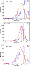 |
Fig. 1. Histogram of the number of sources in filters V and I in NGC 1326A, NGC 1425, and NGC 4548. The blue and red dashed vertical lines correspond to the magnitude in V and I, respectively, where our sample reaches 50% completeness. |
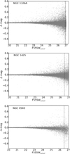 |
Fig. 2. Difference between input and output magnitudes as a function of the output magnitude for NGC 1326A, NGC 1425, and NGC 4548. The dashed line indicates the 50% completeness magnitude. |
3. Massive star population
3.1. Identification of the massive star candidates
We examined the massive star population in each field using color and magnitude criteria to determine the blue, yellow, and red supergiant regions. Figures 3–5 show the V − I versus MV CMD for the stars that passed the quality tests mentioned in Sect. 2, based on the distance modulus of each field (see Table 5). The error bars shown were derived from the artificial star tests. The total foreground interstellar reddening is E(V − I) = 0.15 ± 0.04 mag in NGC 1326A, E(V − I) = 0.16 ± 0.03 mag in NGC 1425, and E(V − I) = 0.18 ± 0.04 mag in NGC 4548 (Freedman et al. 2001). The faint limit in each field corresponds to the V magnitude up to which our sample reaches 50% completeness, as at this magnitude the photometric errors do not exceed 0.1 mag. We adopted the color and magnitude criteria described by Grammer & Humphreys (2013) to separate the regions of BSG, YSGs, and RSGs. The three populations for each field are listed below.
| NGC 1326A | ||
| BSGs | (V − I) ≤ 0.25 mag | 21.5 ≤ V ≤ 25.5 mag |
| (V − I) ≤ 0.60 mag | 25.5 < V ≤ 26.8 mag | |
| YSGs | 0.25 < (V − I) ≤ 0.6 mag | 21.5 ≤ V ≤ 25.5 mag |
| 0.6 < (V − I) ≤ 1.3 mag | 21.5 < V ≤ 26.8 mag | |
| RSGs | (V − I) > 1.3 mag | 21.5 ≤ V ≤ 26.8 mag |
| NGC 1425 | ||
| BSGs | (V − I) ≤ 0.25 mag | 21.5 ≤ V ≤ 25.3 mag |
| (V − I) ≤ 0.60 mag | 25.3 < V ≤ 26.9 mag | |
| YSGs | 0.25 < (V − I) ≤ 0.6 mag | 21.5 ≤ V ≤ 25.3 mag |
| 0.6 < (V − I) ≤ 1.3 mag | 21.5 < V ≤ 26.9 mag | |
| RSGs | (V − I) > 1.3 mag | 21.5 ≤ V ≤ 26.9 mag |
| NGC 4548 | ||
| BSGs | (V − I) ≤ 0:25 mag | 20.5 ≤ V ≤ 24.5 mag |
| (V − I) ≤ 0.60 mag | 24.5 < V ≤ 26.5 mag | |
| YSGs | 0.25 < (V − I) ≤ 0.6 mag | 20.5 ≤ V ≤ 24.5 mag |
| 0.6 < (V − I) ≤ 1.3 mag | 20.5 < V ≤ 26.5 mag | |
| RSGs | (V − I) > 1.3 mag | 20.5 ≤ V ≤ 26.5 mag |
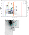 |
Fig. 3. Top panel: V − I vs. V color–magnitude diagram of NGC 1326A. Both absolute and mean magnitudes of the stars are plotted on the y-axis, based on the distance modulus 31.04 mag. The constant stars are shown in gray, the known Cepheids as blue triangles, and the new candidate variables as black dots. Bottom panel: spatial distribution of the candidate variable sources in NGC 1326A. |
In total we identified 7640 candidate BSGs (2652 in NGC 1326A, 2833 NGC 1425, and 2155 in NGC 4548), 2314 candidate YSGs (868 in NGC 1326A, 939 in NGC 1425, and 507 in NGC 4548), and 4270 candidate RSGs (1868 in NGC 1326A, 1281 in NGC 1425, and 1121 in NGC 4548).
We estimated the foreground contamination in the direction of the three fields through the Besançon Galactic population synthesis model (Robin et al. 2003) and found that the majority of the foreground stars lie in the YSG and RSG regions. Foreground contamination has always been a challenge in identifying luminous massive stars such as YSGs and RSGs because these types of stars have similar magnitudes as Milky Way stars. Photometric errors near the completeness limits could also cause contamination, for example, by YSGs that are part of the neighboring RSG population, through reddening and extinction.
Table 4 lists the properties (inclination, distance, distance modulus, metallicity, mophological type, redshift, and absolute magnitude) of NGC 1326A, NGC 1425, and NGC 4548. Table 5 includes the galaxy name, the numbers of candidate BSGs, YSGs, and RSGs, along with those of their variable counterparts. As shown in Table 5, the galaxy with the highest foreground contamination is NGC 4548, followed by NGC 1425 and NGC 1326A.
Properties of NGC 1326A, NGC 1425, and NGC 4548.
Massive star population in NGC 1326A, NGC 1425, and NGC 4548.
3.2. Blue to red supergiant ratio
We calculated the deprojected distances of the luminous stars with respect to the center of each field and took the inclination angle of each galaxy into account (see Table 5). We split the massive stars into three groups: BSGs, YSGs, and RSGs, based on the color and magnitude criteria described in Sect. 3.1. We set ten annuli of equal distance from the center of the galaxy, normalized the number of BSGs, YSGs, and RSGs to the same area taking the foreground contamination of each field into account, and propagated the related errors to calculate the B/R. The spatial distribution of the BSGs and RSGs within the annuli in each field is shown in the right column of Fig. 6. The left column of Fig. 6 shows the trend of the B/R versus galactocentric radius in NGC 1326A, NGC 1425, and NGC 4548. The B/R in all galaxies declines radially, indicating an evident drop of the number of BSGs at the outer regions of the field. The exponential decline of the B/R in the first panel of Fig. 6 is misleading because it is basically caused by the first data point that corresponds to the center of NGC 1326A, which is included in the image of the galaxy. In NGC 4548 the B/R shows a decreasing trend with a rise in the number of blue supergiants that occurs at the sixth annulus (1.43′). This arises because the annulus coincides with the spiral arm of the field, where more BSGs are located because high gas and dust accumulate. A declining B/R with increasing radius has been reported by previous studies (Humphreys & Sandage 1980; Eggenberger et al. 2002; Spetsieri et al. 2018) and has been linked with the radial changes of the metallicity of the field. We compared our results on the B/R with our previous study and the study of Grammer & Humphreys (2013) for NGC 1326A, NGC 1425, and NGC 4548, and assumed that the center of the galaxy is the region with the highest metallicity. The variation of the number of blue to red supergiants with metallicity is a test for stellar evolutionary models because it is highly linked with star formation events and star formation history (Langer 2012). In areas with small coverage, variations in the B/R can occur due to photometric errors and reddening in the outer regions of the field, but we have eliminated this possibility because we normalized our distances to the center of each field using galactic coordinates. The increase of metallicity with galactocentric radius is therefore less likely to be due to systematic errors caused by reddening and photometry.
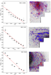 |
Fig. 6. Left column: blue to red supergiant ratio for NGC 1326A, NGC 1425, and, NGC 4548. The dashed red line is a linear fit indicating the monotonic radial decline of the blue to red supergiants. Right column: spatial distribution of the blue and red supergiants. The radius of each of the white annuli displayed shows the distance with respect to the center of each galaxy. |
Our results are in agreement with our previous work on the massive star population in the Virgo cluster galaxy NGC 4535 in Paper I and in M101 (Grammer & Humphreys 2013). The observations of M101 (Grammer & Humphreys 2013) covered the whole galaxy, while in this study, the WFPC2 field of view only covered about a quarter of the galaxy. However, the radial decline of the B/R with decreasing metallicity is common in all fields, confirming the trend that has been presented by previous studies (Eggenberger et al. 2002; Maeder et al. 1980).
3.3. Luminosity function and star formation rate
We used the Modules for Experiments in Stellar Astrophysics (MESA) Isochrones and Stellar Tracks (Choi et al. 2016, MIST) at the metallicity of each galaxy (see Table 5) to estimate the evolutionary state of the massive stars. We used the method described in Dohm-Palmer et al. (1997) to derive the V luminosity function for the blue helium-burning stars (blue HeB stars) in NGC 1326A, NGC 1425, and NGC 4548. For each field we set magnitude bins of equal magnitude (0.18 mag) from MV = − 3.8 up to −9 mag for NGC 1326A, NGC 1425, and NGC 4548 (i.e., the magnitude where the sample reaches 50% completeness). The models indicate sources within the age of 5–100 Myr. The luminosity function of the blue HeB stars in the V band in all three fields is plotted in Fig. 7 (right column). The errors were derived by the artificial star tests, while error propagation has also been used from one bin to another. The numbers plotted above the luminosity function are the ages of the isochrones in megayears based on the MESA models. In order to estimate the SFR based on the counts given from the luminosity function, we made use of the equation given in Dohm-Palmer et al. (1997),
 (1)
(1)
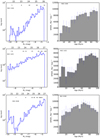 |
Fig. 7. Left column: SFR in M⊙ Myr−1 kpc−2 for NGC 1326A, NGC 1425, and NGC 4548 over the last 100 Myr, based on the blue HeB stars. The blue HeB luminosity function has been normalized to account for the IMF and the changing lifetime in this phase with mass. We used the Salpeter IMF slope and the MESA evolutionary tracks. Right column: luminosity function of the blue HeB stars in NGC 1326A, NGC 1425, and NGC 4548. The bin width is 0.18 mag. The uncertainties in magnitude are derived by the artificial star tests. Plotted above the histogram is the age in megayears for the blue HeB stars as given by the MESA models. |
adjusted for the stars, where ϕ is the initial mass function (IMF) normalized to unity, m is mass, R is the SFR in units of M⊙ yr−1, and t is time. We used the Salpeter slope for the IMF, and the normalized IMF is
 (2)
(2)
For each galaxy we derived the area of the filed of view of our observations to determine the SFR/kpc2. The SFR/kpc2 is shown in Fig. 7.
The star formation history of NGC 1326A shows a gradual increase in look-back time at M⊙ kpc−2, indicating high SFRs over the past 70 Myr. In NGC 1425 the star formation history reveals a recent peak ∼10 Myr followed by a drop, which could be a sign of a star formation event. The high number of YSGs in NGC 1425 presented in Table 5 could explain a star formation event over which massive stars formed and evolved simultaneously. The SFR appears constant between 25–40 Myr and increases between 40–70 Myr. From 70–100 Myr on, the star formation history does not vary significantly. The field with the highest is the Virgo cluster galaxy NGC 4548. The SFR in NGC 4548 indicates a constant increase with small fluctuations between 5 and 65 Myr; the SFR reaches its peak at 9000 M⊙ kpc−2 at 70 Myr. Between 75 and 100 Myr, the SFR shows a slight decrease. NGC 4548 has the highest estimated metallicity of the three fields. This could be an indication of how star formation proceeds as a function of metallicity because the role of massive stars in star formation remains unclear. The recent star formation history estimated for the three fields does not show signs of significant star burst events that could result in the formation of 100 M⊙ stars. Because massive stars are characterized by their brief lifetimes, we do not rule out the existence of stars more massive than 30 M⊙ because they may have evolved and exploded by the time of the observations. Additionally, very young massive stars are born in highly contaminated star-forming regions. As a result, resolving these stars photometrically is challenging because they may appear as diffuse or blended sources.
4. Variability
After identifying the massive stars in the three fields, our next step was to investigate whether these sources displayed any type of variability. We adopted the methodology described in Paper I and considered only the stars with more than five measurements in either the V or I filters. We used the three variability indexes described in Paper I: the median absolute deviation (MAD), the interquartile range (IQR), and the inverse von Neumann ratio (1/η) (Sokolovsky et al. 2017).
The variability indexes were measured in each of the WFPC2 chips in all three fields. To derive the variability indexes, we sorted the sources included in each WFPC2 chip by increasing magnitude and set bins with at least 5% of the total number of sources per bin to maintain statistical significance. For each bin, we calculated the median value of the index and the standard deviation (σ), we set a 4σ threshold and considered as variable candidates all sources above that threshold in either F555W or F814W. Figure 8 shows an example of the index versus magnitude diagram for the MAD in the WF3 chip of WFPC2 in the V filter for NGC 1326A, NGC 1425, and NGC 4548. Candidate variable sources are shown as red squares, and the known Cepheids are shown as blue triangles. All published Cepheid variables in all three fields were recovered by our algorithm. We created index versus magnitude plots for all chips in all three galaxies and determined the final number of variables.
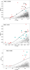 |
Fig. 8. Mean absolute deviation vs. mean magnitude for the WF3 chip in NGC 1326A, NGC 1425, and NGC 4548. The dashed line shows the stars over the 4σ threshold. The variable candidates are shown as red squares and the known variables are shown as blue triangles. |
The total number of new variable candidates is 243, which are distributed as follows: 48 variable candidates in NGC 1326A, 102 in NGC 1425, and 93 in NGC 4548. We present light curves for all the new variable candidates we identified in Figs. A.1–A.3. The figures show that the variable candidates vary with the same trend in both filters and display variations of similar amplitude. Tables 6–8 contain the full list with IDs, coordinates, mean magnitude, magnitude errors, variability indexes, HSC v3 MatchIDs, and notes of the variables in all three fields. The tables also include the amplitude of variability and classification based on their V − I color and mass as estimated by the models. In Tables 6–8 we use digit 1 to flag the sources that appeared variable in any of the three variability indexes and digit 0 for the sources that were not selected as variables by an index. When a star is flagged as variable in only one index and filter, we assume that this might be due to the wavelength dependence of variability or due to the sensitivity of the index to the type of the variability displayed.
Among the variable sources that were primarily detected by the algorithm were the published Cepheids of the three fields. In particular, there were 15 reported Cepheids in NGC 1326A, 20 in NGC 1425, and 24 in NGC 4548. These sources are not included in Tables 6–8 because they are known sources, but we used the mean magnitudes by Prosser et al. (1999), Mould et al. (2000), Graham et al. (1999) to test the quality of our photometry. We found a negligible discrepancy between the latter studies and our measurements. The differences in magnitude are 0.015 ± 0.004 mag for NGC 1326A, 0.033 ± 0.009 mag for NGC 1425, and 0.018 ± 0.006 mag for NGC 4548.
All variables in all three fields were identified by MAD in at least one filter, while 211 out of 243 variables were detected in at least one filter in IQR. The inverse von Neumann ratio index is more sensitive to correlation-based than to scatter-based observations, and 37% of the variable candidates were selected by this index.
We used MESA evolutionary tracks to estimate the masses of the new variables in each field. The models were generated assuming rotation at 40% of the critical speed and values of metallicity for each field based on Freedman et al. (2001). We adopted solar metallicity for NGC 1326A and supersolar values for metallicity for NGC 1425 and NGC 4548. Figures 3–5 show both the CMDs and finder charts of the new candidate variables and evolutionary tracks overplotted along with the spatial distribution of the candidate variable stars for each galaxy, respectively. The masses corresponding to the tracks span from ∼8−20 M⊙ and the magnitude ranges from −3.8 mag to −9 mag. The error bars correspond to the uncertainty due to reddening E(V − I), photometric errors, and the distance modulus. We took the E(V − I) reddening in each field into account, derived the reddening vector based on the E(V − I) values mentioned in Sect. 3.1, and adopted a ratio of total to selective absorption RV = AV/(AV − AI) = 3.1 (Cardelli et al. 1989; Freedman et al. 2001). The evolutionary tracks shown in each plot correspond to 8, 10, 15, and 20 M⊙ for the metallicities implied by Freedman et al. (2001). The degeneracy of the evolutionary tracks of different M⊙ does not allow us to reliably estimate the mass of the candidate massive stars. For example, in Fig. 5 the 8 M⊙ track overlaps the 10 M⊙ track, making it challenging to distinguish stars within that mass range. However, the mass range proposed for the candidate massive stars seems fully compliant with the values of metallicity and extinction of each field.
Based on the colors (V − I) and mass range of the published variables shown in Fig. 3–5, we proceeded to classify the newly discovered candidate massive variable stars. In the three fields, the new candidate variables lie between ∼8−20 M⊙, while in NGC 1326A, 17 out of the 48 newly identified candidate variables display masses below 8 M⊙. The majority of the variable stars in the fields show V − I colors between −0.5 and 2.5 mag. The CMD in Fig. 3 displays fewer candidate massive variable stars than the CMDs in Figs. 4 and 5. This is explained by the different parts of each galaxy that are covered during the observations of the HST Key Project. In NGC 1425 and NGC 4548 the observations cover a larger part of the spiral arms than in NGC 1326A. The subsections below provide information about the new variable candidate BSGs, YSGs, and RSGs that we identified in the three galaxies.
4.1. Candidate variable red supergiants
Our analysis yielded 21 candidate variable RSGs, 3 in NGC 1326A, 6 in NGC 1425, and 10 in NGC 4548. The magnitude range of the candidates is −7.0 ≤ MV ≤ − 4.0 mag, and the V − I index is within 1.6−2.1 mag. According to the MESA models, the masses and temperatures of the stars are between 8 and 16 M⊙ and 3000 < Teff < 4000 K. However, stars between 7 M⊙ and 8 M⊙ may also be super-AGB stars (Becker & Iben 1980; Groenewegen & Sloan 2018). Super-AGB stars are equally luminous to RSGs and with a similar color, making it difficult to distinguish sources of these two types given the uncertainty in distance. The basic feature used to identify RSGs is their bolometric magnitude (Mbol ≤ − 7.1 mag) (Wood et al. 1983). However, stars with MV < − 7 mag with masses above 16 M⊙ are less likely to be super-AGB stars.
Although most RSGs do not usually show variability or periodic variability, the candidate RSGs in the three fields vary in both filters, and in some cases display amplitudes between 0.2 and 0.6 mag. The studies of Yang & Jiang (2012) and Yang et al. (2018) reported a periodic variability of the RSGs in the LMC and SMC, but in our case, it is difficult to define a period for the light curve of the candidate RSGs because of the short timescale and the few observations. Based on the studies of Levesque et al. (2006), Szczygieł et al. (2010), and Yang et al. (2018), claiming periodic variability in RSGs is more robust with many observations and a long timescale. In our work, the amplitude of the light variation is between 0.2 − 0.6 ± 0.03 mag over ∼100 days. Variability in red supergiants has many underlying causes such as radial pulsations (Wood et al. 1983; Stothers 1969; Heger et al. 1997) photospheric changes, huge convection cells (Schwarzschild 1975; Antia et al. 1984) mass transfer, and stellar winds.
4.2. Candidate variable yellow supergiants or hypergiants
Among the massive stars of our sample are 12 variable candidate YSGs. The stars show MV brighter than −5 mag, while the models imply masses and temperatures in the range 15 < M < 20 M⊙ and 5900 < Teff < 7500 K. They also display a variation in their light curve in both filters within a short timescale. The galaxy with most candidate variable YSGs is NGC 1425, which also contains most candidate variable stars. The YSG region is often affected by foreground contamination. In our study, foreground contamination occurs between 0.8 < V − I < 1.3 mag. YSGs belong to the most visually luminous stars, with absolute magnitude MV reaching −9 mag, evolving from the main sequence towards the RSG state, or following the opposite path (Humphreys et al. 2016). Another short evolutionary state of post-RSGs with masses between 20 − 40 M⊙ is the yellow hypergiant phase (YHGs) (de Jager 1998). YHGs display temperatures ranging between 4000 and 7000 K and log L/L⊙ > 5.4 and are characterized by atmospheric instability and extended turbulent structures. During the YHG phase, massive stars undergo high mass-losses that are shed as expanding pseudo-photospheric shells. These sources are among the SN type IIn progenitors (Smith 2014), which makes their identification and observational follow-up valuable. The brightest source in the YSG region is V1 in NGC 1425, which displays MV ∼ − 9 mag, ∼30 M⊙ and Teff ∼ 7000 K. Based on its characteristics, this source is classified as a candidate variable YSG/YHG. Variability in YSGs has previously been reported in the studies of Humphreys & Davidson (1979), Percy & Kim (2014), Humphreys et al. (2016), Kourniotis et al. (2017), Spetsieri et al. (2018) in the region with M⊙ ≥ 20 M⊙ and log L/L⊙ > 5.4. and is typical of amplitude 0.3–0.6 mag similar to the amplitude of V1. As spectroscopic classification is essential for accurate distinction between YHGs and YSGs, we cannot further infer on the state of our yellow stars.
4.3. Candidate variable blue supergiants
Among the candidate variable massive stars identified in the three fields are eight blue supergiants. We expect no foreground contamination in this region according to the Besançon models. The mass range implied by the models for the candidate variable BSGs is 15–20 M⊙, the magnitudes range between −8 < MV < −4.9 mag, and the temperatures, based on the models, range from 5900 < Teff < 17400 K. The field with most BSGs (64) is the Virgo cluster galaxy NGC 4548. As shown in Sect. 3.3, this galaxy is considered to be forming stars. The variability amplitude of the BSGs reaches 1.2 mag for the low-mass candidate BSGs (e.g., V97 in NGC 1425) and 0.1 mag for brighter and more massive BSGs (e.g., V7 in NGC 1425).
The existence of many BSGs in a galaxy is indicative of recent star formation because BSGs are young stellar objects that are found in the galactic spiral arms in regions that are rich in gas and dust. Based on stellar evolution theory (Ekström et al. 2012) a star in the BSG region might either come directly from the main sequence to the supergiant region or might return to higher temperatures before central helium exhaustion after the RSG phase. In order to distinguish whether a source in the BSG region is evolving redward after the main sequence or is undergoing a blue loop, the internal mixing in the radiative layers, the strength of stellar winds (if evident), and the metallicity are required. Variability of BSGs, and in particular pulsations of such sources, has been used as a diagnostic tool for the evolutionary stages before and after helium-core ignition (Ostrowski & Daszyńska-Daszkiewicz 2015). Kraus et al. (2015) studied the blue supergiant 55 Cygnus over a five-year baseline to link its pulsational activity with mass-loss episodes and the formation of clumps in the stellar wind.
To summarize, we identified extragalactic candidate variable BSGs, and reported their variability over a short baseline of ∼100 days. Because BSGs are pre-collapse SN progenitors, large amplitude variations in their light curves could be indicative of an unstable stage before stellar death.
4.4. New candidate periodic variables
We conducted a period search to define the periodic variable sources in all three fields (see Table 8). We identified four Cepheid variables in NGC 1425 within a time-baseline of 100 days. We estimated the period of the variable sources based on their light curve, using the online tool of the NASA Exoplanet Archive3. The periods estimated for the periodic variables range from 25 to 60 days and are marked in Table 7. The periodic variables are located in the YSG region between 8 and 9 M⊙ near the known Cepheids of each field, that is, the instability strip (Sandage & Tammann 1971; Macri et al. 1999). Their magnitude and color ranges are −4 < MV < − 5 mag and 0.5 < V − I < 1.2 mag. The light curves of all sources (Fig. A.3) show pulsations similar to the Cepheid variables. They are shown as yellow stars in the CMD in Fig. 4. We propose follow-up photometric observations to better identify the nature of these sources.
5. Summary
We performed PSF photometry on archival HST WFPC2 images and created a catalog of luminous stars for the HST Key project galaxies NGC 1326A, NGC 1425, and NGC 4548. In all three fields we studied the massive star population and created three separate subcatalogs of massive stars with MV < −4.0 mag. In particular, the number of massive stars identified in each field are 5388 in NGC 1326A, 5053 in NGC 1425, and 3783 in NGC 4548. Using color criteria on the CMD, we separated the massive star candidates into three subsets: BSGs, YSGs, and RSGs. We calculated the foreground contamination in the direction of each galaxy using the Besançon Galactic population synthesis model. The region with the lowest foreground contamination in the three galaxies is the BSG region. The percentage of foreground stars in that region is ∼1.3% in NGC 1326A, ∼0.8% in NGC 1425, and ∼3.7% in NGC 4548. The region that is most affected by foreground contamination is the YSG region, with ∼25% in NGC 1326A, ∼29% in NGC 1425, and ∼30% in NGC 4548 being foreground stars.
We calculated the deprojected distances of the massive stars and estimated the blue to red supergiant ratio at various radial distances for the three galaxies. The B/R decreases monotonically with increasing distance and decreasing metallicity. We examined the recent star formation history of the field over the last 100 Myr within the WFPC2 field of view. We derived the luminosity function based on the blue HeB stars and estimated the SFR using the Salpeter slope for the IMF. NGC 4548 includes most stars and has a higher SFR than NGC 1326A and NGC 1425. The star formation history of NGC 1326A shows an increase, indicating high SFRs over the past 70 Myr. In NGC 1425 the star formation history has a recent peak at ∼10 Myr, which is an indication of a star formation event.
We conducted a variability search among 5789 sources in NGC 1326A, 5232 sources in NGC 1425, and 5790 sources in NGC 4548 using three different methods: the MAD, IQR, and the inverse von Neumann ratio. The number of stars used for the variability search includes all sources that fulfilled the quality criteria mentioned in Sect. 2.2. The number of stars in Table 5 implies the massive stars in each field. The variability search yielded 243 new variable sources in addition to the 87 known Cepheid variables in the three galaxies. We used the MESA models and evolutionary tracks to model our results and classify the new variable candidates. Among the luminous massive variable sources are 138 variable candidate BSGs, 86 variable candidate YSGs, and 19 variable candidate RSGs. In addition to the candidate variable massive stars, we identified four periodic variable candidates in NGC 1425, which we suggest for follow-up observations.
This work provides a census of the massive star population and variable massive stars in three HST Key Project galaxies using archival data from the Hubble Legacy Archive (HLA). Future work on the massive star population in distant fields using the combination of deep HST data and high-precision PSF photometry will shed light on the link of massive stars with the galactic star formation history. Increasing the number of photometric and spectroscopic observations of massive stars could help identify SN Type II progenitors and constrain the evolutionary models of massive stars. Thereby, important information about their properties and evolution will be unveiled.
Acknowledgments
We would like to thank the anonymous referee for the insightful comments that helped improve this paper. We acknowledge financial support by the European Space Agency (ESA) under the “Hubble Catalog of Variables” program, contract no. 4000112940. This research has made use of the VizieR catalog access tools, CDS, Strasbourg, France and NASA’s Astrophysics Data System (ADS). The Virtual Observatory tools (VO) TOPCAT (Taylor 2005) and Aladin were used for image downloading and table manipulation. The data used in this study were downloaded from the Mikulski Archive for Space Telescopes (MAST). All figures in this work were produced using Matplotlib a Python library for publication graphics.
References
- Anderson, J., & King, I. R. 2000, PASP, 112, 1360 [NASA ADS] [CrossRef] [Google Scholar]
- Antia, H. M., Chitre, S. M., & Narasimha, D. 1984, ApJ, 282, 574 [NASA ADS] [CrossRef] [Google Scholar]
- Becker, S. A., & Iben, Jr., I. 1980, ApJ, 237, 111 [NASA ADS] [CrossRef] [Google Scholar]
- Bonanos, A. Z. 2007, AJ, 133, 2696 [NASA ADS] [CrossRef] [Google Scholar]
- Brunish, W. M., Gallagher, J. S., & Truran, J. W. 1986, AJ, 91, 598 [NASA ADS] [CrossRef] [Google Scholar]
- Cardelli, J. A., Clayton, G. C., & Mathis, J. S. 1989, ApJ, 345, 245 [NASA ADS] [CrossRef] [Google Scholar]
- Choi, J., Dotter, A., Conroy, C., et al. 2016, ApJ, 823, 102 [NASA ADS] [CrossRef] [Google Scholar]
- Conroy, C., Strader, J., van Dokkum, P., et al. 2018, ApJ, 864, 111 [NASA ADS] [CrossRef] [Google Scholar]
- de Jager, C. 1998, A&ARv, 8, 145 [NASA ADS] [CrossRef] [Google Scholar]
- Dohm-Palmer, R. C., Skillman, E. D., Saha, A., et al. 1997, AJ, 114, 2527 [NASA ADS] [CrossRef] [Google Scholar]
- Dolphin, A. E. 2000, PASP, 112, 1383 [NASA ADS] [CrossRef] [Google Scholar]
- Eggenberger, P., Meynet, G., & Maeder, A. 2002, A&A, 386, 576 [NASA ADS] [CrossRef] [EDP Sciences] [Google Scholar]
- Ekström, S., Georgy, C., Eggenberger, P., et al. 2012, A&A, 537, A146 [NASA ADS] [CrossRef] [EDP Sciences] [Google Scholar]
- Freedman, W. L., Madore, B. F., Gibson, B. K., et al. 2001, ApJ, 553, 47 [NASA ADS] [CrossRef] [Google Scholar]
- Graham, J. A., Ferrarese, L., Freedman, W. L., et al. 1999, ApJ, 516, 626 [NASA ADS] [CrossRef] [Google Scholar]
- Grammer, S., & Humphreys, R. M. 2013, AJ, 146, 114 [NASA ADS] [CrossRef] [Google Scholar]
- Groenewegen, M. A. T., & Sloan, G. C. 2018, A&A, 609, A114 [NASA ADS] [CrossRef] [EDP Sciences] [Google Scholar]
- Heger, A., & Langer, N. 2000, ApJ, 544, 1016 [NASA ADS] [CrossRef] [Google Scholar]
- Heger, A., Jeannin, L., Langer, N., & Baraffe, I. 1997, A&A, 327, 224 [NASA ADS] [Google Scholar]
- Humphreys, R. M., & Davidson, K. 1979, ApJ, 232, 409 [NASA ADS] [CrossRef] [Google Scholar]
- Humphreys, R. M., & Sandage, A. 1980, ApJS, 44, 319 [NASA ADS] [CrossRef] [Google Scholar]
- Humphreys, R. M., Martin, J. C., Gordon, M. S., & Jones, T. J. 2016, ApJ, 826, 191 [NASA ADS] [CrossRef] [Google Scholar]
- Kalari, V. M., Vink, J. S., Dufton, P. L., & Fraser, M. 2018, A&A, 618, A17 [NASA ADS] [CrossRef] [EDP Sciences] [Google Scholar]
- Kochanek, C. S., Fraser, M., Adams, S. M., et al. 2017, MNRAS, 467, 3347 [NASA ADS] [CrossRef] [Google Scholar]
- Kourniotis, M., Bonanos, A. Z., Yuan, W., et al. 2017, A&A, 601, A76 [NASA ADS] [CrossRef] [EDP Sciences] [Google Scholar]
- Kraus, M., Haucke, M., Cidale, L. S., et al. 2015, A&A, 581, A75 [NASA ADS] [CrossRef] [EDP Sciences] [Google Scholar]
- Langer, N. 2012, ARA&A, 50, 107 [NASA ADS] [CrossRef] [Google Scholar]
- Langer, N., & Maeder, A. 1995, A&A, 295, 685 [NASA ADS] [Google Scholar]
- Levesque, E. M., Massey, P., Olsen, K. A. G., et al. 2006, ApJ, 645, 1102 [NASA ADS] [CrossRef] [Google Scholar]
- Lianou, S., & Cole, A. A. 2013, A&A, 549, A47 [NASA ADS] [CrossRef] [EDP Sciences] [Google Scholar]
- Macri, L. M., Huchra, J. P., Stetson, P. B., et al. 1999, ApJ, 521, 155 [NASA ADS] [CrossRef] [Google Scholar]
- Maeder, A., & Meynet, G. 2000, A&A, 361, 159 [NASA ADS] [Google Scholar]
- Maeder, A., Lequeux, J., & Azzopardi, M. 1980, A&A, 90, L17 [NASA ADS] [Google Scholar]
- Massey, P. 2003, ARA&A, 41, 15 [NASA ADS] [CrossRef] [Google Scholar]
- Moriya, T. J. 2018, MNRAS, 475, L49 [NASA ADS] [CrossRef] [Google Scholar]
- Mould, J. R., Huchra, J. P., Freedman, W. L., et al. 2000, ApJ, 545, 547 [NASA ADS] [CrossRef] [Google Scholar]
- Ostrowski, J., & Daszyńska-Daszkiewicz, J. 2015, MNRAS, 447, 2378 [NASA ADS] [CrossRef] [Google Scholar]
- Percy, J. R., & Kim, R. Y. H. 2014, J. Am. Assoc. Variable Star Observers (JAAVSO), 42, 267 [NASA ADS] [Google Scholar]
- Prieto, J. L., Stanek, K. Z., Kochanek, C. S., et al. 2008, ApJ, 673, L59 [NASA ADS] [CrossRef] [Google Scholar]
- Prosser, C. F., Kennicutt, Jr., R. C., Bresolin, F., et al. 1999, ApJ, 525, 80 [NASA ADS] [CrossRef] [Google Scholar]
- Robin, A. C., Reylé, C., Derrière, S., & Picaud, S. 2003, A&A, 409, 523 [NASA ADS] [CrossRef] [EDP Sciences] [Google Scholar]
- Sandage, A., & Tammann, G. A. 1971, ApJ, 167, 293 [NASA ADS] [CrossRef] [Google Scholar]
- Schwarzschild, M. 1975, ApJ, 195, 137 [NASA ADS] [CrossRef] [Google Scholar]
- Smith, N. 2014, ARA&A, 52, 487 [NASA ADS] [CrossRef] [MathSciNet] [Google Scholar]
- Sokolovsky, K. V., Gavras, P., Karampelas, A., et al. 2017, MNRAS, 464, 274 [NASA ADS] [CrossRef] [Google Scholar]
- Soraisam, M. D., Gilfanov, M., Kupfer, T., et al. 2018, A&A, 615, A152 [NASA ADS] [CrossRef] [EDP Sciences] [Google Scholar]
- Spetsieri, Z. T., Bonanos, A. Z., Kourniotis, M., et al. 2018, A&A, 618, A185 [NASA ADS] [CrossRef] [EDP Sciences] [Google Scholar]
- Stothers, R. 1969, ApJ, 156, 541 [NASA ADS] [CrossRef] [Google Scholar]
- Szczygieł, D. M., Stanek, K. Z., Bonanos, A. Z., et al. 2010, AJ, 140, 14 [NASA ADS] [CrossRef] [Google Scholar]
- Taylor, M. B. 2005, in Astronomical Data Analysis Software and Systems XIV, eds. P. Shopbell, M. Britton, & R. Ebert, ASP Conf. Ser., 347, 29 [Google Scholar]
- Whitmore, B. C., Allam, S. S., Budavári, T., et al. 2016, AJ, 151, 134 [NASA ADS] [CrossRef] [Google Scholar]
- Wood, P. R., Bessell, M. S., & Fox, M. W. 1983, ApJ, 272, 99 [NASA ADS] [CrossRef] [Google Scholar]
- Yang, M., & Jiang, B. W. 2012, ApJ, 754, 35 [NASA ADS] [CrossRef] [Google Scholar]
- Yang, M., Bonanos, A. Z., Jiang, B.-W., et al. 2018, A&A, 616, A175 [NASA ADS] [CrossRef] [EDP Sciences] [Google Scholar]
Appendix A: Additional figures
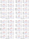 |
Fig. A.1. Light curves of the candidate variables in NGC 1326A. The V filter is shown as filled blue circles and the I filter as red squares. |
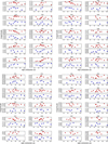 |
Fig. A.2. continued. |
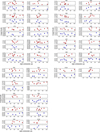 |
Fig. A.2. continued. |
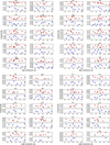 |
Fig. A.3. continued. |
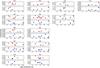 |
Fig. A.3. continued. |
All Tables
All Figures
|
Fig. 1. Histogram of the number of sources in filters V and I in NGC 1326A, NGC 1425, and NGC 4548. The blue and red dashed vertical lines correspond to the magnitude in V and I, respectively, where our sample reaches 50% completeness. |
| In the text | |
|
Fig. 2. Difference between input and output magnitudes as a function of the output magnitude for NGC 1326A, NGC 1425, and NGC 4548. The dashed line indicates the 50% completeness magnitude. |
| In the text | |
|
Fig. 3. Top panel: V − I vs. V color–magnitude diagram of NGC 1326A. Both absolute and mean magnitudes of the stars are plotted on the y-axis, based on the distance modulus 31.04 mag. The constant stars are shown in gray, the known Cepheids as blue triangles, and the new candidate variables as black dots. Bottom panel: spatial distribution of the candidate variable sources in NGC 1326A. |
| In the text | |
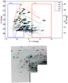 |
Fig. 4. Same as Fig. 3 for NGC 1425. |
| In the text | |
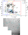 |
Fig. 5. Same as Fig. 3 for NGC 4548. |
| In the text | |
|
Fig. 6. Left column: blue to red supergiant ratio for NGC 1326A, NGC 1425, and, NGC 4548. The dashed red line is a linear fit indicating the monotonic radial decline of the blue to red supergiants. Right column: spatial distribution of the blue and red supergiants. The radius of each of the white annuli displayed shows the distance with respect to the center of each galaxy. |
| In the text | |
|
Fig. 7. Left column: SFR in M⊙ Myr−1 kpc−2 for NGC 1326A, NGC 1425, and NGC 4548 over the last 100 Myr, based on the blue HeB stars. The blue HeB luminosity function has been normalized to account for the IMF and the changing lifetime in this phase with mass. We used the Salpeter IMF slope and the MESA evolutionary tracks. Right column: luminosity function of the blue HeB stars in NGC 1326A, NGC 1425, and NGC 4548. The bin width is 0.18 mag. The uncertainties in magnitude are derived by the artificial star tests. Plotted above the histogram is the age in megayears for the blue HeB stars as given by the MESA models. |
| In the text | |
|
Fig. 8. Mean absolute deviation vs. mean magnitude for the WF3 chip in NGC 1326A, NGC 1425, and NGC 4548. The dashed line shows the stars over the 4σ threshold. The variable candidates are shown as red squares and the known variables are shown as blue triangles. |
| In the text | |
|
Fig. A.1. Light curves of the candidate variables in NGC 1326A. The V filter is shown as filled blue circles and the I filter as red squares. |
| In the text | |
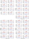 |
Fig. A.2. Same as Fig. A.1, but for NGC 1425. |
| In the text | |
|
Fig. A.2. continued. |
| In the text | |
|
Fig. A.2. continued. |
| In the text | |
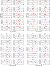 |
Fig. A.3. Same as Fig. A.1, but for NGC 4548. |
| In the text | |
|
Fig. A.3. continued. |
| In the text | |
|
Fig. A.3. continued. |
| In the text | |
Current usage metrics show cumulative count of Article Views (full-text article views including HTML views, PDF and ePub downloads, according to the available data) and Abstracts Views on Vision4Press platform.
Data correspond to usage on the plateform after 2015. The current usage metrics is available 48-96 hours after online publication and is updated daily on week days.
Initial download of the metrics may take a while.