| Issue |
A&A
Volume 629, September 2019
|
|
|---|---|---|
| Article Number | A74 | |
| Number of page(s) | 11 | |
| Section | Numerical methods and codes | |
| DOI | https://doi.org/10.1051/0004-6361/201935937 | |
| Published online | 06 September 2019 | |
The LUMBA UVES stellar parameter pipeline
1
Observational Astrophysics, Division of Astronomy and Space Physics, Department of Physics and Astronomy, Uppsala University, Box 516, 75120 Uppsala, Sweden
e-mail: This email address is being protected from spambots. You need JavaScript enabled to view it.
2
Max Planck Institute for Astronomy (MPIA), Koenigstuhl 17, 69117 Heidelberg, Germany
3
Research School of Astronomy and Astrophysics, Australian National University, Canberra, ACT 2611, Australia
4
ARC Centre of Excellence for All Sky Astrophysics in 3 Dimensions (ASTRO 3D), Australia
Received:
22
May
2019
Accepted:
10
July
2019
Abstract
Context. The Gaia-ESO Survey has taken high-quality spectra of a subset of 100 000 stars observed with the Gaia spacecraft. The goal for this subset is to derive chemical abundances for these stars that will complement the astrometric data collected by Gaia. Deriving the chemical abundances requires that the stellar parameters be determined.
Aims. We present a pipeline for deriving stellar parameters from spectra observed with the FLAMES-UVES spectrograph in its standard fibre-fed mode centred on 580 nm, as used in the Gaia-ESO Survey. We quantify the performance of the pipeline in terms of systematic offsets and scatter. In doing so, we present a general method for benchmarking stellar parameter determination pipelines.
Methods. Assuming a general model of the errors in stellar parameter pipelines, together with a sample of spectra of stars whose stellar parameters are known from fundamental measurements and relations, we use a Markov chain Monte Carlo method to quantitatively test the pipeline.
Results. We find that the pipeline provides parameter estimates with systematic errors on effective temperature below 100 K, on surface gravity below 0.1 dex, and on metallicity below 0.05 dex for the main spectral types of star observed in the Gaia-ESO Survey and tested here. The performance on red giants is somewhat lower.
Conclusions. The pipeline performs well enough to fulfil its intended purpose within the Gaia-ESO Survey. It is also general enough that it can be put to use on spectra from other surveys or other spectrographs similar to FLAMES-UVES.
Key words: methods: numerical / stars: atmospheres / stars: statistics
© ESO 2019
1. Introduction
The Gaia spacecraft is currently making high-precision parallax measurements to determine positions and proper motions, together with spectroscopic radial velocity determinations, for astronomical objects in and around the Milky Way. To date, the Gaia sample contains more than 1.7 billion objects (Gaia Collaboration 2018). Between 2012 and 2018, the Gaia-ESO Survey (GES) has performed complementary ground-based observations, taking high-resolution spectra of a subset of about one hundred thousand Gaia stars, together with some stars too bright to be observed by Gaia. These spectra are being used to derive chemical abundances for the GES stars. The intent is for the Gaia astrometric data and the GES chemical data to be used together to study the history of the Milky Way, and by extension galactic evolution in general (Gilmore et al. 2012).
As an initial step in determining chemical abundances for the stars, it is necessary to determine their stellar parameters. For GES, this requires pipelines that automatically perform the determination. This is partly because the sheer number of spectra precludes manual fitting of model spectra, but also because it promotes reproducibility and homogeneity. A spectroscopist who has performed manual fitting of a handful of spectra can hopefully account for the process for each one, but this cannot reasonably be done for thousands of individual spectra. If a data set were to be split between several spectroscopists for manual fitting, the results would also be split into as many clusters with their own systematic errors due to the idiosyncrasies of each individual spectroscopist’s fitting process. Since the GES data will be used for statistical analyses, avoiding this clustering becomes more important.
Several different stellar parameter determination pipelines are used within GES. Different pipelines have to be used for spectra observed with different spectrographs, and for different regions of parameter space. In addition, a number of different pipelines are used on the same samples of spectra. This is done partly to increase the accuracy of the derived parameters since it decreases the impact of the assumptions and approximations going into any particular pipeline. Furthermore, the scatter from pipeline to pipeline provides the most robust way of estimating the error on the derived parameters, although it cannot catch systematic errors coming from assumptions and approximations shared by all (Smiljanic et al. 2014).
Spectra observed with the UVES spectrograph (see Sect. 2) are analysed in 13 groups called nodes, each of which has its own pipeline. An outline of the pipelines is given in Smiljanic et al. (2014). The pipelines use the codes ARES (Sousa et al. 2007), BACCHUS (Masseron et al. 2016), DAOSPEC (Stetson & Pancino 2008), FAMA (Magrini et al. 2013), FERRE, GALA (Mucciarelli et al. 2013), GAUFRE (Valentini et al. 2013), MATISSE (Recio-Blanco et al. 2006), MyGIsFOS (Sbordone et al. 2014), ROTFIT (Frasca et al. 2003, 2006), SME (Piskunov & Valenti 1996, 2017) and StePar (Tabernero et al. 2013). This paper documents the SME-based pipeline used by the Lund-Uppsala-MPIA-Bordeaux-ANU (LUMBA) node.
The portion of the GES sample analysed with this pipeline contains 6941 spectra, excluding the spectra that are used in benchmarking the pipeline. The median S/N is 60. The central 90% of the S/N values for the sample fall in the range 17–180. We plot the current best GES estimates of Teff and log g, colour-coded by S/N in Fig. 1. These estimates are a homogenisation of estimates produced by several groups within GES, including LUMBA.
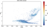 |
Fig. 1. Spectra analysed with the pipeline described in this paper. The stellar parameters given are the best estimates arrived at by several groups within GES. The spectra are colour-coded according to S/N. Where stars overlap, those with highest S/N have been placed on top. |
The paper is organised as follows. Section 2 gives a brief overview of the characteristics of the observational material collected as part of GES. Section 3 describes the pipeline itself. Section 4 discusses the performance of the pipeline. Section 5 summarises our findings.
2. Observations with FLAMES-UVES
The Fibre Large Array Multi Element Spectrograph (FLAMES) is a spectrograph installed on the VLT UT2 telescope (Pasquini et al. 2002). It feeds the red arm of the two-arm cross-dispersed echelle spectrograph called Ultraviolet and Visual Echelle Spectrograph (UVES; Dekker et al. 2000).
The spectra used here have a resolution of around R ≡ λ/δλ = 47 000, and are taken with the RED580 setting, which covers the wavelength range of 4760 Å–6840 Å, with a 50 Å gap in the middle due to the physical gap between the two detectors making up the UVES red arm (Sbordone & Ledoux 2018).
3. Pipeline
The pipeline is based on the LUMBA pipeline for spectra taken with the GIRAFFE spectrograph. They differ in a number of ways, including modifications to make use of the higher resolution and different wavelength range of the UVES. It has been used, in different versions, in the internal GES data releases iDR5 and iDR6. It is similar to the pipeline for the GALAH spectrograph, which is also based on the LUMBA pipeline for GIRAFFE (Buder et al. 2018).
3.1. Algorithm
Based on an observed spectrum, the pipeline attempts to fit a synthetic spectrum by varying the following parameters:
-
Teff: effective temperature;
-
log g: surface gravity;
-
[Fe/H]: metallicity;
-
v sin i: projected rotational speed of stellar equator;
-
vmic: microturbulence parameter;
-
[Ca/Fe]: calcium abundance;
-
[Mg/Fe]: magnesium abundance.
Since the macroturbulence parameter vmac tends to be almost fully degenerate with v sin i, it is given a separate treatment, described in Appendix A. The fitting is done over discrete segments in the spectrum, which have been selected to contain spectral lines that constrain each parameter. This is described in detail in Sect. 3.2. When running, the pipeline goes through the following four steps:
-
Preliminary normalisation of all segments;
-
Preliminary determination of all parameters, performing at most 2 iterations of the fitting algorithm;
-
Final normalisation of all segments;
-
Final determination of all parameters, performing at most 20 iterations of the fitting algorithm.
This is done using a number of pre-existing software tools, described in Sect. 3.3.
3.2. Line selection
Our choice of lines is based on classical spectroscopic techniques to constrain the main stellar parameters Teff, log g, [Fe/H], and additional parameters like v sin i and vmic (see e.g. Gray 2005). However, the goodness-of-fit metric used in the fitting treats all lines equivalently. This means that to the extent that a line has any sensitivity at all to a parameter, it will contribute to the estimate of that parameter. The spectral lines analysed in the pipeline fall into six groups, each of which is intended to predominantly constrain a single stellar parameter:
-
Strong neutral calcium lines, which are sensitive to log g and the calcium abundance;
-
Weak neutral calcium lines, which are sensitive to the calcium abundance but not log g;
-
Strong neutral magnesium lines, which are sensitive to log g and the magnesium abundance;
-
A set of neutral iron lines, which are sensitive to [Fe/H];
-
A set of singly ionised iron lines, which are sensitive to log g and [Fe/H].
The weak lines of calcium and magnesium are intended to break the degeneracy in the strong lines between log g and the abundances. There are no separate lines for Teff, v sin i, and vmic since they affect all lines in ways that are not degenerate with the other parameters. While the calcium and magnesium lines are mainly of interest for their usefulness in determining log g, the derived abundances can also be used to identify stars with discrepant chemical compositions (departure of α-elements as seen in the thick disk and the halo), even before any detailed abundance analysis has been done.
The lines were selected from the GES line list, based on the quality of their measured transition probabilities and blending properties (Heiter et al. 2015a, 2019). This is described in Sect. 3.3.2. The analysis uses line and segment masks, which is explained in Sect. 3.3.1. We give a full list of the lines in Appendix B.
3.3. External software
The central piece of external software in the pipeline is the spectral synthesis code SME. This in turn requires the GES line list, a grid of model atmospheres, and grids of non-local thermodynamic equilibrium (NLTE) departure coefficients.
The pipeline is written in Interactive Data Language (IDL) and makes extensive use of functions from the IDL Astronomy User’s Library (IDLAstro) and the Coyote IDL library (Landsman 1993; Fanning 2015).
3.3.1. Spectroscopy Made Easy
Spectroscopy Made Easy (SME) is a code for computing synthetic spectra on the fly, which can be used against observed spectra to automatically fit stellar parameters and/or chemical abundances. It was originally published in 1996. Since then it has been substantially expanded and improved (Piskunov & Valenti 1996, 2017). At the time of writing the pipeline uses SME version 542, and we plan to update it as new versions are released.
When fitting a spectrum, SME requires the user to define segment masks, continuum masks, and line masks. The segment masks specify which wavelength regions are to be considered at all. Outside, no synthesis and no fitting is performed. The continuum masks specify the regions within each segment that are assumed to be close to the continuum, which is used by SME to normalise the segments. The line masks state the regions within each segment over which the fitting is to be performed (Piskunov et al. 2016). Since they are susceptible to chromospheric contributions and deviations from local thermodynamic equilibrium (LTE), the cores of strong lines are left out of the fit, as described in Appendix C.
SME can normalise an observed spectrum, using any of several procedures. In our case, it is done by rescaling each individual segment under the assumption that the continuum is locally linear. The scaling is done by minimising a Pearson’s χ2 sum between the observed and modelled intensities over the pixels covered by the continuum mask (Piskunov et al. 2016). We note that the model spectrum that is computed for the normalisation includes spectral lines. This means that even if spectral lines happen to be covered by the continuum mask, it is possible to get a useful normalisation as long as those lines are included in the line list. The inaccuracy in the normalisation then depends on how close the stellar parameters used to compute the model spectrum are to the correct values. By alternately fitting stellar parameters and normalising, it is then possible to get good estimates of both. If the continuum mask covers lines not included in the line list, on the other hand, it will lead to the continuum being incorrectly fitted. We use the automated algorithm described in Appendix D, which determines a suitable continuum mask for each observed spectrum and segment and takes into account blending and accuracy criteria.
When deriving stellar parameters, SME attempts to minimise a pseudo-χ2 sum, defined as
 (1)
(1)
where Oi is the observed intensity in pixel i, Ei is the modelled intensity in the same pixel, σi is the uncertainty in the observed intensity, and the sum runs over all pixels contained within the line masks. The minimisation is done using a version of the Levenberg-Marquardt algorithm, adapted to the modified χ2 sum (Levenberg 1944; Marquardt 1963; Piskunov & Valenti 2017). The additional factor of Oi, which is not present in a conventional χ2 sum, causes SME to prefer placing the model spectrum above the observed spectrum than to placing it below. This reflects a heuristic commonly used by spectroscopists when fitting spectra manually; the main source of error in a synthetic spectrum often comes from the incompleteness of the line list. This means that a perfect choice of stellar parameters should produce a model spectrum lying slightly above the observed spectrum (Piskunov, priv. comm.).
Accurately determining errors in fitted stellar parameters is still an unsolved problem. Most error estimations assume that the main source of error is statistical errors on the input data. This is almost never the case for spectral fitting, where the error is typically dominated by systematic errors on the model. SME versions from 433 onwards use a heuristic method for estimating the error that tries to take systematics into account. All pixels i in the line mask with a non-zero partial derivative of the model flux Fi with respect to the parameter p are chosen. Of the chosen pixels, those with a residual Ri between the observed and the best-fit model spectrum that is less than five times the measurement uncertainty are then selected. Under the assumption that the model intensity is locally linear, the change Δp needed to make the residual zero is given by
 (2)
(2)
This gives a distribution of Δp-values. The width of this distribution is taken to be the 68% of values around the centre. This width is then taken to be the best estimate of the parameter uncertainty (Piskunov & Valenti 2017). This method seems to overestimate the errors by a factor of a few, but it is still useful as an order-of-magnitude estimate.
The fitting procedure requires a set of starting values for the stellar parameters. As long as the masks are chosen so that the problem is not close to being degenerate, these starting values will generally only affect the time needed for the fitting to converge on a solution, and will not affect the final result (Piskunov & Valenti 2017). The only exception is radial velocity, for which it is necessary to supply a good starting estimate (Piskunov, priv. comm.). For GES spectra this is usually irrelevant, since most of them have been corrected for radial velocity. The starting values used for the other parameters in the pipeline are generally the best estimates given in the internal data releases of GES. The exception is the microturbulence parameter vmic, which together with the fixed macroturbulence parameter vmac is given the treatment described in Appendix E. The abundance pattern is initially assumed to be the same as in the Sun, although rescaled based on the starting value of [Fe/H] (Piskunov et al. 2016). In the pipeline, the individual abundances for calcium and magnesium are free parameters since lines of those elements are used to estimate log g.
3.3.2. GES line list
To compute spectra, SME needs a list specifying the wavelength, oscillator strength, and other line parameters for the spectral lines thought to be relevant. For this pipeline we used the GES line list, which was developed to enable homogeneous analysis with high-quality line data within GES. It contains the best literature values of the line parameters for 1341 transitions.
Before the line and segment masks were defined, the reliability of the atomic data and their degree of blending with other lines were both classified into three categories of decreasing quality: Y, U, and N. The atomic data was classified according to the assumed reliability of the literature values. Recent precise laboratory measurements were classified as Y. Older less precise laboratory measurements were classified as U. Semi-empirical calculations were classified as N. The blending was classified by comparing model spectra to reference spectra for the Sun and Arcturus. Lines only blended with lines of the same species in both stars were classified as Y. Lines blended to some extent with other species in at least one of the stars were classified as U. Lines strongly blended with other species in both stars were classified as N (Heiter et al. 2015a, 2019). The line and segment masks were then defined, when possible, by selecting lines of quality Y in both respects. When a line type only had a few available lines, lines of quality U in either reliability or blending, but not both, were permitted.
3.3.3. MARCS model atmospheres
To compute spectra, SME needs a grid of model atmospheres over the relevant ranges of Teff, log g, and [Fe/H]. For our pipeline we use a grid calculated by Bengt Edvardsson using the Model Atmospheres with a Radiative and Convective Scheme (MARCS) code, within the ranges 4000 K < Teff < 8000 K, −0.5 < log g < 5.0, −5.0 < [Fe/H] < 1.0.
MARCS has been in use in different versions since the 1970s, and a standardised version was published in 2008. It computes model atmospheres for late-type stars under the assumptions of plane-parallel or spherical symmetry, hydrostatic equilibrium, mixing-length convection treatment, and LTE (Gustafsson et al. 2008).
3.3.4. NLTE grids
While the MARCS model atmospheres were computed under the assumption of LTE radiative transfer, SME performs spectrum synthesis taking into account pre-computed grids of NLTE departure coefficients for certain elements (Piskunov & Valenti 2017). At present, the pipeline uses departure coefficients only for iron (Bergemann et al. 2012; Lind et al. 2012).
4. Performance
We now attempt to evaluate how well the pipeline performs in practice. Since the pipeline is mainly used within GES for statistical analysis of large samples of stars, we are mostly interested in the systematic offsets in the derived parameters. These offsets are expected to differ somewhat depending on the type of star. For our purposes, we consider that the pipeline performs well for a type of star as long as the offset in Teff is below 100 K, the offset in log g is below 0.1 dex, and the offset in [Fe/H] is below 0.05 dex. These offsets are somewhat arbitrarily chosen, but reflect requirements from science cases related to Galactic chemical evolution.
The most straightforward way of estimating the offsets is by using the pipeline to derive stellar parameters of stars for which the correct values are already known. We have a sample of such stars called the “Gaia FGK benchmark stars”, widely used within GES for this purpose (Blanco-Cuaresma et al. 2014; Heiter et al. 2015b). As an additional sanity check, we test the pipeline on the open cluster M 67, comparing the derived stellar parameters to stellar isochrones.
4.1. Comparison to benchmark stars
For the Gaia FGK benchmark stars, Teff and log g have been estimated from fundamental observations and relations, such as direct measurements of angular diameters, astrometric parallax, and the bolometric flux. This makes the estimates independent of the assumptions made in spectral modelling (Blanco-Cuaresma et al. 2014; Heiter et al. 2015b). The benchmark stars used in this paper are were chosen to be representative of four types of stars, referred to as
-
Solar-type stars;
-
F dwarfs;
-
FGK subgiants;
-
Red giants.
For the first three types, we used all of the GES benchmark stars available. For the red giants, we removed all stars with Teff < 4000 K since they fall outside of our grid of atmospheres. We also disregarded the star HD 122563, which our pipeline is unable to analyse. We believe that this occurs because the star both is a red giant and has a metallicity of [Fe/H] = −2.64, the lowest of all benchmark stars. Stars with very low metallicity are in general difficult to analyse spectroscopically since the low value decreases the depth of spectral lines. Red giants are also difficult to analyse with this particular pipeline, for reasons we discuss below. In Table 1, we list the benchmark stars used together with the number of spectra available for each star.
Benchmark stars.
The benchmark spectra have been observed using the ESPaDOnS, NARVAL, and UVES spectrographs and convolved to a resolution of 47 000, matching that of FLAMES-UVES (Blanco-Cuaresma et al. 2014). For these spectrographs the gaps in the spectra do not overlap with the segments used in our analysis. However, the wavelength gap around 5306–5337 Å in the HARPS benchmark spectra contains several FeĨI lines used in our analysis, which has forced us to avoid those spectra. The spectral files come from the Blanco-Cuaresma library in Blanco-Cuaresma (2019).
Using the method described in Appendix F, we estimated the systematic offsets for each parameter and type of star. We show our best estimates in Table 2. We note that unfortunately it is not possible to directly compare the performance to that of similar pipelines. The method for estimating performance was developed for this paper, and has not yet been used on other pipelines.
Estimated systematic offsets for benchmark stars.
We show the mean offset for each individual star, averaged over all spectra of that star, for Teff in Fig. 2, for log g in Fig. 3, and for [Fe/H] in Fig. 4.
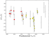 |
Fig. 2. Unweighted mean offset for Teff for benchmark stars. Error bars denote the standard deviation in the mean added in quadrature to the uncertainty in the fundamental-parameter estimate provided in Heiter et al. (2015b). The yellow hexagram denotes the Sun. Yellow circles denote other solar-type stars. White circles denote F dwarfs. Yellow squares denote FGK subgiants. Red squares denote red giants. |
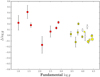 |
Fig. 3. Unweighted mean offset for log g for benchmark stars. Error bars denote the standard deviation in the mean added in quadrature to the uncertainty in the fundamental-parameter estimate provided in Heiter et al. (2015b), the other symbols as in Fig. 2. |
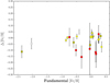 |
Fig. 4. Unweighted mean offset for [Fe/H] for benchmark stars. Error bars denote the standard deviation in the mean added in quadrature to the uncertainty in the fundamental-parameter estimate provided in Heiter et al. (2015b), the other symbols as in Fig. 2. |
As can be seen, the pipeline generally performs satisfactorily, with systematic offsets in Teff below 100 K, in log g below 0.1 dex, and in [Fe/H] below 0.05 dex. The only exception is the group of red giants for which the average offsets in log g and [Fe/H] are estimated to be 0.15 ± 0.03 dex and −0.07 ± 0.05 dex, respectively. We believe that this is partly due to the increased line density at lower temperatures causing line blending, which makes the continuum determination difficult. However, since red giants differ the most from the stars used for testing during the early development of the pipeline, it may be that they conform less to other implicit assumptions built into the pipeline. We note that the tendency is to overestimate log g for red giants, which is the opposite of what usually results from LTE-based stellar parameter determinations.
4.2. Comparison to M 67 isochrones
While benchmark stars give the most reliable and easily interpreted tests of a stellar parameter pipeline, it is possible to also use stellar clusters for additional sanity checks. We chose the old open cluster M 67 (NGC 2682) for this. This cluster is well studied in the literature and contains stars with a wide span of stellar parameters, including the solar twin YBP 1194 (Önehag et al. 2011) and some blue stragglers.
We have access to 42 UVES spectra of stars in the field of the cluster, all of which come from the GES sample. Of these, 20 were observed in 2004 within project 072.D-0309(A) with principal investigator C.H.F. Melo, and 22 were observed in 2009 within project 082.D-0726(A) with principal investigator B. Gustafsson. All of the spectra are in the ESO archive, and reprocessed spectra will be made available after the final GES data release. The stellar parameters derived by LUMBA, and the other nodes mentioned in Sect. 1, will be included in the final GES data release.
Based on the description in the SIMBAD database, we listed some of the stars as “red giant”, “variable”, “binary”, and “blue straggler” (Wenger et al. 2000). The spectra also include the solar twin YBP-1194. This could in principle be a very useful reference star since it has been repeatedly studied over the past few years (Liu et al. 2016). Unfortunately, there are known problems with the spectra of this star taken with FLAMES-UVES (Önehag et al. 2011). We list the coordinates for these stars in Table G.1, together with our classification.
We compare the derived Teff and log g to isochrones with appropriately chosen metallicity and age, and look for trends in [Fe/H] as a function of log g. The cluster isochrones were calculated using PARSEC v1.2S and COLIBRI S35 using version 3.2 of the web input form1 (Marigo et al. 2017). We calculated isochrones for ages 3.5 Gy and 4.8 Gy since the true age is believed to lie somewhere within this range. We took the metallicity to be 0.06 dex (Önehag et al. 2014).
We show the Teff and log g estimates and isochrones in Fig. 5. Visually, the agreement looks good. The only stars that are noticeably far off from the isochrone are the blue straggler, two binary star systems, and one variable star. However, it is difficult to make any quantitative statement of how good the agreement is. We note that the estimates on average fall within 0.6σ of the closest points on the two isochrones, but this metric cannot be easily turned into an estimate of the parameter offsets. To calculate the likelihood of getting a particular set of estimates, assuming certain values of the parameter offsets requires us to have a well-defined prior for both the cluster age and the positions on the isochrone. For a detailed discussion of the problems with comparing isochrones to data, see Valls-Gabaud (2014).
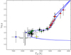 |
Fig. 5. Estimates of Teff and log g for stars in M 67. Error bars denote the errors returned by SME. The yellow circle denotes the solar twin YBP-1194. Blue circles denote blue stragglers. Green circles denote variable stars. White circles denote binary stars. Red circles denote red giants. Black circles denote other stars. The blue curves denote isochrones calculated for the highest and lowest age estimates for the cluster. One star with σTeff > 500 K has not been included. |
The estimates of [Fe/H] have a weighted mean of −0.02 ± 0.02 dex, which is somewhat lower than the assumed cluster [Fe/H]. This mean is independent of whether red giants are included or not. However, the cluster [Fe/H] was adopted from Önehag et al. (2014) after correcting for the effects of atomic diffusion. Considering this, our [Fe/H] estimate for the main-sequence, turn-off, and subgiant stars agrees with Önehag et al. (2014).
We plot the estimated [Fe/H] as a function of the estimated log g together with a Deming regression in Fig. 6. There is an apparent trend in [Fe/H], but it is only significant if red giants are included in the fit. The trend is not what is expected from atomic diffusion and thus contradicts recent findings (Souto et al. 2019). Given the above discussions on the performance of the pipeline on red-giant spectra, we do not believe that this trend reflects the true iron trend in M 67. Similar difficulties with analysing red giants were seen when M 67 was studied with the related GALAH pipeline (Gao et al. 2018).
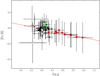 |
Fig. 6. Estimates of log g and [Fe/H] for stars in M 67. Error bars denote the errors returned by SME. The yellow circle denotes YBP-1194. Blue circles denote blue stragglers. Green circles denote variable stars. White circles denote binary stars. Red circles denote red giants. Black circles denote other stars. The red line denotes the best-fit line given by the Deming regression. One star with σTeff > 500 K has not been included. |
5. Summary
As part of the work within GES, the LUMBA collaboration has developed a pipeline for deriving stellar parameters from spectra observed with FLAMES-UVES or similar spectrographs. The pipeline uses the spectral synthesis code SME to do the fitting, together with the GES line list, a grid of MARCS model atmospheres, NLTE grids, and commonly used IDL libraries. The best-fit parameters are determined by minimising a χ2-like sum.
We developed a method for estimating the systematic offsets for stellar parameter pipelines by testing them on the spectra of benchmark stars with stellar parameters estimated from fundamental observations and relations. Using this method reveals systematic offsets in Teff below 100 K, in log g below 0.1 dex, and in [Fe/H] below 0.05 dex for the most common GES targets. The performance is somewhat degraded for red giants. We comment on the difficulties of using stellar clusters as quantitative tests of pipeline performance. The achieved level of accuracy makes the pipeline suitable for applications in the framework of studies of Galactic chemical evolution.
Acknowledgments
We wish to commemorate our colleague and friend Gregory Ruchti (1980–2019) who originally branched off this pipeline from the LUMBA-internal GIRAFFE pipeline. We thank the GES team for the work behind the M 67 spectra and for making them available to us. We thank Caroline Soubiran, Paula Jofré, and Maria Bergemann for contributions to the work behind the pipeline. AG, UH, and AJK acknowledge support from the Swedish National Space Agency and the Knut and Alice Wallenberg Foundation. Parts of this research were conducted by the Australian Research Council Centre of Excellence for All Sky Astrophysics in 3 Dimensions (ASTRO 3D), through project number CE170100013. PG thanks the European Science Foundation (ESF) for support in the framework of EuroGENESIS. KL acknowledges funds from the Alexander von Humboldt Foundation in the framework of the Sofja Kovalevskaja Award endowed by the Federal Ministry of Education and Research and funds from the Swedish Research Council (Grant no. 2015-00415_3) and Marie Skłodowska Curie Actions (Cofund Project INCA 600398). This research has made use of the SIMBAD database, operated at CDS, Strasbourg, France.
References
- Bergemann, M., Lind, K., Collet, R., Magic, Z., & Asplund, M. 2012, MNRAS, 427, 27 [NASA ADS] [CrossRef] [Google Scholar]
- Blanco-Cuaresma, S. 2019, The Gaia FGK Benchmark Stars, https://www.blancocuaresma.com/s/benchmarkstars [Google Scholar]
- Blanco-Cuaresma, S., Soubiran, C., Jofré, P., & Heiter, U. 2014, A&A, 566, A98 [NASA ADS] [CrossRef] [EDP Sciences] [Google Scholar]
- Buder, S., Asplund, M., Duong, L., et al. 2018, MNRAS, 478, 4513 [NASA ADS] [CrossRef] [Google Scholar]
- Dekker, H., D’Odoric, S., Kaufer, A., Delabre, B., & Kotzlowski, H. 2000, in Optical and IR Telescope Instrumentation and Detectors, Proc. SPIE, 4008 [Google Scholar]
- Fanning, D. W. 2015, Coyote’s Guide to IDL Programming, http://www.idlcoyote.com/ [Google Scholar]
- Foreman-Mackey, D., Hogg, D. W., Lang, D., & Goodman, J. 2013, PASP, 125, 306 [CrossRef] [Google Scholar]
- Frasca, A., Alcalá, J. M., Covino, E., et al. 2003, A&A, 405, 149 [NASA ADS] [CrossRef] [EDP Sciences] [Google Scholar]
- Frasca, A., Guillout, P., Marilli, E., et al. 2006, A&A, 454, 301 [NASA ADS] [CrossRef] [EDP Sciences] [Google Scholar]
- Gaia Collaboration (Brown, A. G. A., et al.) 2018, A&A, 616, A1 [NASA ADS] [CrossRef] [EDP Sciences] [Google Scholar]
- Gao, X., Lind, K., Amarsi, A. M., et al. 2018, MNRAS, 481, 2666 [NASA ADS] [CrossRef] [Google Scholar]
- Gilmore, G., Randich, S., Asplund, M., et al. 2012, The Messenger, 147, 25 [NASA ADS] [Google Scholar]
- Gray, D. F. 2005, The Observation and Analysis of Stellar Photospheres, 3rd edn. (Cambridge: Cambridge University Press) [CrossRef] [Google Scholar]
- Gustafsson, B., Edvardsson, B., Eriksson, K., et al. 2008, A&A, 486, 951 [NASA ADS] [CrossRef] [EDP Sciences] [Google Scholar]
- Heiter, U., Lind, K., Asplund, M., et al. 2015a, Phys. Scr., 90, 054010 [Google Scholar]
- Heiter, U., Jofré, P., Gustafsson, B., et al. 2015b, A&A, 582, A49 [NASA ADS] [CrossRef] [EDP Sciences] [PubMed] [Google Scholar]
- Heiter, U., Lind, K., Bergemann, M., et al. 2019, A&A, submitted [Google Scholar]
- Landsman, W. B. 1993, in Astronomical Data Analysis Software and Systems II, eds. R. J. Hanisch, R. J. V. Brissenden, & J. Barnes, ASP Conf. Ser., 52, 246 [NASA ADS] [Google Scholar]
- Levenberg, K. 1944, Q. Appl. Math., 2, 164 [Google Scholar]
- Lind, K., Bergemann, M., & Asplund, M. 2012, MNRAS, 427, 50 [NASA ADS] [CrossRef] [Google Scholar]
- Liu, F., Asplund, M., Yong, D., et al. 2016, MNRAS, 463, 696 [NASA ADS] [CrossRef] [Google Scholar]
- Magrini, L., Randich, S., Friel, E., et al. 2013, A&A, 558, A38 [NASA ADS] [CrossRef] [EDP Sciences] [Google Scholar]
- Marigo, P., Girardi, L., Bressan, A., et al. 2017, ApJ, 835, 77 [NASA ADS] [CrossRef] [Google Scholar]
- Marquardt, D. W. 1963, J. Soc. Ind. Appl. Math., 11, 431 [Google Scholar]
- Masseron, T., Merle, T., & Hawkins, K. 2016, Astrophysics Source Code Library [record ascl:1605.004] [Google Scholar]
- Mucciarelli, A., Pancino, E., Lovisi, L., Ferraro, F. R., & Lapenna, E. 2013, ApJ, 766, 78 [NASA ADS] [CrossRef] [Google Scholar]
- Önehag, A., Korn, A., Gustafsson, B., Stempels, E., & VandenBerg, D. A. 2011, A&A, 528, A85 [NASA ADS] [CrossRef] [EDP Sciences] [Google Scholar]
- Önehag, A., Gustafsson, B., & Korn, A. 2014, A&A, 562, A102 [NASA ADS] [CrossRef] [EDP Sciences] [Google Scholar]
- Pasquini, L., Avila, G., Blecha, A., et al. 2002, The Messenger, 110, 1 [Google Scholar]
- Piskunov, N. E., & Valenti, J. A. 1996, A&AS, 118, 595 [NASA ADS] [CrossRef] [EDP Sciences] [Google Scholar]
- Piskunov, N. E., & Valenti, J. A. 2017, A&A, 597, A16 [NASA ADS] [CrossRef] [EDP Sciences] [Google Scholar]
- Piskunov, N. E., Valenti, J. A., & Heiter, U. 2016, Spectroscopy Made “Easy” (SME) User Handbook [Google Scholar]
- Recio-Blanco, A., Bijaoui, A., & de Laverny, P. 2006, MNRAS, 370, 141 [NASA ADS] [CrossRef] [Google Scholar]
- Sbordone, L., & Ledoux, C. 2018, Very Large Telescope Paranal Science Operations UV-Visual Echelle Spectrograph User manual, 102nd edn., Karl-Schwarzschild Str. 2, D-85748 Garching bei München [Google Scholar]
- Sbordone, L., Caffau, E., Bonifacio, P., & Duffau, S. 2014, A&A, 564, A109 [NASA ADS] [CrossRef] [EDP Sciences] [Google Scholar]
- Smiljanic, R., Korn, A. J., Bergemann, M., et al. 2014, A&A, 570, A122 [NASA ADS] [CrossRef] [EDP Sciences] [Google Scholar]
- Sousa, S. G., Santos, N. C., Israelian, G., Mayor, M., & Monteiro, M. J. P. F. G. 2007, A&A, 469, 783 [NASA ADS] [CrossRef] [EDP Sciences] [Google Scholar]
- Souto, D., Allende Prieto, C., Cunha, K., et al. 2019, ApJ, 874, 97 [NASA ADS] [CrossRef] [Google Scholar]
- Stetson, P. B., & Pancino, E. 2008, PASP, 120, 1332 [Google Scholar]
- Tabernero, H. M., González Hernández, J. I., & Montes, D. 2013, in Highlights of Spanish Astrophysics VII, eds. J. C. Guirado, L. M. Lara, V. Quilis, & J. Gorgas, 673 [Google Scholar]
- Valenti, J. A., & Fischer, D. A. 2005, ApJS, 159, 141 [NASA ADS] [CrossRef] [MathSciNet] [Google Scholar]
- Valentini, M., Morel, T., Miglio, A., Fossati, L., & Munari, U. 2013, Eur. Phys. J. Web Conf., 43, 03006 [CrossRef] [Google Scholar]
- Valls-Gabaud, D. 2014, EAS Publ. Ser., 65, 225 [CrossRef] [EDP Sciences] [Google Scholar]
- Wenger, M., Ochsenbein, F., Egret, D., et al. 2000, A&AS, 143, 9 [NASA ADS] [CrossRef] [EDP Sciences] [Google Scholar]
Appendix A: Treatment of vmac
For most spectra, v sin i and vmac are too degenerate to be determined separately. Hence, it is common to have a single parameter that essentially stands in for the combined effect of the two parameters. This is done in e.g. Valenti & Fischer (2005).
In our pipeline we define such a parameter, which we refer to here as v sin ipseudo. The starting value of v sin ipseudo, start is taken by adding the estimate of vmac to the starting guess of the pure v sin i in quadrature. Meanwhile vmac is treated as being zero in the code:

After the fitting is finished, the best estimate v sin ifinal is taken by subtracting in quadrature the estimated vmac (see Appendix E) from the final estimate of v sin ipseudo.

Appendix B: Lines
We show the full list of lines in Table B.1. The “line mask” columns give the wavelength ranges used in the fitting. The “segment” columns give the wavelength ranges of the segments that make up the synthetic spectra.
Line masks.
Appendix C: Cores of strong lines
Even with the NLTE grids described in Sect. 3.3.4, SME cannot reliably model the NLTE-dominated cores of strong lines. Hence, the pipeline automatically removes from the line mask every pixel within 4 Å of the line centre where the modelled flux falls below a threshold. The threshold intensity is denoted cmin and is given by
![Mathematical equation: $$ \begin{aligned} c_\text{ min}&\equiv \left\{ \begin{array}{l} 0.60, \qquad -1 < \left[ \text{ Fe} / \text{ H} \right] \\ 0.65, \qquad -2 < \left[ \text{ Fe} / \text{ H} \right] < -1 \\ 0.72, \qquad \qquad \;\left[ \text{ Fe} / \text{ H} \right] < -2 \end{array}. \right. \end{aligned} $$](/articles/aa/full_html/2019/09/aa35937-19/aa35937-19-eq5.gif) (C.1)
(C.1)
Appendix D: Continuum mask
The segment and line masks are defined ahead of time. Instead, the continuum masks are defined algorithmically for each segment when the pipeline is run. The algorithm attempts to find continuum points by avoiding those points (based on the line list) that are known to be parts of lines, or (based on the observed spectrum) that appear to be parts of either telluric lines or stellar lines missing from the line list. To do this we define the parameter cfrac that is used to determine the minimum observed intensity a pixel must have to be included in the continuum mask. We also define the parameter cwt that is used to determine the minimum model intensity a pixel must have to be included in the mask. Finally, we define the parameter efrac that defines the maximum observed intensity a pixel must have to be included in the mask. This is intended to remove atmospheric emission lines.
The algorithm is defined as follows: First a preliminary normalisation is done of each segment by robustly fitting a straight line to the highest points in the observed spectrum, using the robust_poly_fit routine from the IDLAstro library (Landsman 1993). Then any pixel outside of the line mask will be assigned to the continuum mask if all of the following are true:
-
The observed intensity is among the cfrac + efrac highest;
-
The model intensity is among the cwt ⋅ cfrac + efrac highest;
-
The observed intensity is not among the efrac highest.
If this results in fewer than ten pixels being assigned to the continuum mask in the left one-third or the right one-third of the segment, cfrac is increased enough for that third to include ten pixels.
We note that the choice to compare model pixels based to the product cwt ⋅ cfrac is purely one of convenience. We could just as easily have defined one parameter cfrac, model and required that the model intensity lie among the cfrac, model + efrac brightest. The parameters were defined in this way because a user who wants to increase or decrease the strictness of the algorithm would generally want to increase cfrac and cfrac, model by the same proportion. This way, it is only necessary to change one value to do that.
Empirically, the values producing the best results have been found to be in the vicinity of cfrac = 0.2, efrac = 0.005 and cwt = 3.0.
Appendix E: Turbulence parameters
Instead of explicitly stating a starting guess for vmic, we estimated this from Teff using a relation that was derived empirically within GES. While we do not fit vmac, a fixed value for this is also calculated empirically:
As long as Teff > 5500 K and log g > 4.2, a set of default values of the parameters is used. Otherwise we use a special set of values. We show the values in Table E.1.
Parameters determining  and vmac.
Appendix F: Estimating systematic offsets
We assume that we have N benchmark stars, which we index with i. For each star we have ni benchmark spectra, which we index with k. For each benchmark star and stellar parameter, there is some correct value  . Let
. Let  be the estimate of
  given by fundamental relations. Let pi, k be the estimate of
  given by analysing spectrum k of star i with the pipeline.
We assume that the estimates returned by fundamental relations can be described as the sum of the true value and one error term:
 (F.1)
(F.1)
The term  is assumed to differ from star to star following a normal distribution with mean 0 and standard deviation
  . We take the uncertainties stated in Heiter et al. (2015b) as our estimates of
  . We assume that the estimates returned by the pipeline can be described as the sum of the true value and three error terms:
 (F.2)
(F.2)
The term epipe represents the error due to inherent flaws and limitations in the pipeline. This could come from lines that are incorrectly described in the line list, or that are missing altogether. While this term is parameter-dependent, we assume that it can be treated as constant within some volume of parameter space. The term ei represents the error due to how the pipeline is affected by the peculiarities unique to each star. This could come from blends due to unusual abundances, from difficulties in observing the star that are constant over time, and the like. It is assumed to be constant for all spectra of a particular star, but to vary from star to star following a normal distribution of mean 0 and standard deviation σstar. The term ei, k represents the error due to how the pipeline is affected by the peculiarities of each spectrum. This could come from Poissonian noise, from observational conditions specific to the observation night, and the like. It is assumed to vary from spectrum to spectrum following a normal distribution of mean 0 and standard deviation σspec.
Given these assumptions, the likelihood for a series of estimates {pi, k} is given by
where we have introduced the shorthand
Given a sequence of estimates {pi, k}, a sequence of fundamental estimates  , and a series of uncertainties in the fundamental parameters
  , we can then estimate epipe, σstar, and σspec.
We use Goodman and Weare’s Affine Invariant Markov chain Monte Carlo Ensemble Sampler to estimate the distribution P (Foreman-Mackey et al. 2013). We then use the median of each error parameter as our best estimate of that parameter. We use the 68th percentile as our estimate of the uncertainty in the error parameter.
The resulting estimates of epipe are shown in Table 2. Estimates of all three parameters are shown for Teff in Table F.1, for log g in Table F.2, and for [Fe/H] in Table F.3.
Estimated error parameters for Teff.
Estimated error parameters for log g.
Estimated error parameters for [Fe/H].
While the parameters describing the scatter are reassuringly fairly small, their relative sizes are somewhat discouraging. How well we can determine epipe is limited by σspec and σstar, and by N and ni. If it were the case that σspec = σstar = 0, then a single spectrum of a single benchmark star would be enough to determine epipe exactly. If it were the case that σspec ≫ σstar, then spectrum-to-spectrum scatter would give the main contribution to the error in epipe, which could be dealt with by taking more spectra of each benchmark star. Unfortunately, to within a factor of a few σspec ≈ σstar, which means that to determine epipe much more accurately, we would need to increase the sample of benchmark stars, which is non-trivial. For our fairly rough categorisation of stars into four types, and our assumption that epipe is approximately constant, the number of stars currently available is sufficient. However, if we wanted to estimate the offset over smaller regions of parameter space, either by dividing the benchmark sample into more types of benchmark stars or by replacing the constant epipe with some function of Teff, log g, and [Fe/H], we might not have enough benchmark stars.
Appendix G: M 67 spectra
We show the full list of objects in M 67 for which we have spectra in Table G.1.
Members of the M 67 cluster for which we have spectra.
All Tables
All Figures
|
Fig. 1. Spectra analysed with the pipeline described in this paper. The stellar parameters given are the best estimates arrived at by several groups within GES. The spectra are colour-coded according to S/N. Where stars overlap, those with highest S/N have been placed on top. |
| In the text | |
|
Fig. 2. Unweighted mean offset for Teff for benchmark stars. Error bars denote the standard deviation in the mean added in quadrature to the uncertainty in the fundamental-parameter estimate provided in Heiter et al. (2015b). The yellow hexagram denotes the Sun. Yellow circles denote other solar-type stars. White circles denote F dwarfs. Yellow squares denote FGK subgiants. Red squares denote red giants. |
| In the text | |
|
Fig. 3. Unweighted mean offset for log g for benchmark stars. Error bars denote the standard deviation in the mean added in quadrature to the uncertainty in the fundamental-parameter estimate provided in Heiter et al. (2015b), the other symbols as in Fig. 2. |
| In the text | |
|
Fig. 4. Unweighted mean offset for [Fe/H] for benchmark stars. Error bars denote the standard deviation in the mean added in quadrature to the uncertainty in the fundamental-parameter estimate provided in Heiter et al. (2015b), the other symbols as in Fig. 2. |
| In the text | |
|
Fig. 5. Estimates of Teff and log g for stars in M 67. Error bars denote the errors returned by SME. The yellow circle denotes the solar twin YBP-1194. Blue circles denote blue stragglers. Green circles denote variable stars. White circles denote binary stars. Red circles denote red giants. Black circles denote other stars. The blue curves denote isochrones calculated for the highest and lowest age estimates for the cluster. One star with σTeff > 500 K has not been included. |
| In the text | |
|
Fig. 6. Estimates of log g and [Fe/H] for stars in M 67. Error bars denote the errors returned by SME. The yellow circle denotes YBP-1194. Blue circles denote blue stragglers. Green circles denote variable stars. White circles denote binary stars. Red circles denote red giants. Black circles denote other stars. The red line denotes the best-fit line given by the Deming regression. One star with σTeff > 500 K has not been included. |
| In the text | |
Current usage metrics show cumulative count of Article Views (full-text article views including HTML views, PDF and ePub downloads, according to the available data) and Abstracts Views on Vision4Press platform.
Data correspond to usage on the plateform after 2015. The current usage metrics is available 48-96 hours after online publication and is updated daily on week days.
Initial download of the metrics may take a while.