© J. Wicht et al. 2019

1 Introduction

Two of the main objectives of NASA’s Juno mission are to measure the magnetic field of Jupiter with unprecedented resolution and to determine the depth of the fierce zonal winds observed in its cloud layer. The first Juno-based internal magnetic field model JRM09 (Connerney et al. 2018) already provides the internal magnetic field up to spherical harmonic degree 10 and shows several interesting features that seem unique to the dynamo of Jupiter (Moore et al. 2018). Better-resolved models are expected as the mission continues.

Based on Juno gravity measurements (Iess et al. 2018), Kaspi et al. (2018) deduce that the speed of the equatorially antisymmetric zonal flow contributions must be significantly reduced at a depth of about 3000 km below the one-bar level, which corresponds to a radius of 0.96 r_J. Kong et al. (2018) come to roughly similar conclusions with a different inversion procedure, but they also point out that the solution is not unique. While the gravity data only allow us to constrain the equatorially antisymmetric winds, the results likely also extend to the symmetric contributions. New interior models (Guillot et al. 2018; Debras & Chabrier 2019) and also the width of the dominant equatorial jet (Gastine et al. 2014; Heimpel et al. 2016) both support the idea that the fast zonal winds are roughly confined to the outer 4% in radius.

The fast planetary rotation enforces geostrophic flow structures with minimal variation along the direction of the rotation axis. Geostrophic zonal winds are therefore expected to reach right through the gaseous envelope of the planet, and it remains unclear which mechanism limits their extent in Jupiter. The demixing of hydrogen and helium and the subsequent precipitation of helium deeper into the planet offers one possible explanation (Militzer et al. 2016). This process would have established a helium gradient that suppresses convection. In Jupiter, this stable helium-rain layer may start somewhere between 0.93 and 0.90 r_J and perhaps extends down to 0.80 r_J (Debras & Chabrier 2019). We note however that ab initio simulations by Schöttler & Redmer (2018) predict that the hydrogen/helium demixing may not even have started. Recent analysis of gravity measurements by the Cassini spacecraft suggest that the zonal winds of Saturn may only reach down to about 0.85 r_S (Iess et al. 2019; Galanti et al. 2019). Since the stably stratified layer is thought to start significantly deeper, at about 0.62 r_S according toSchöttler & Redmer (2018), it cannot be the reason for the limited depth of the zonal winds.

A second possible mechanism braking of the zonal winds at depth involves the Lorentz forces. Lorentz forces are tied to dynamo action and thus to the electrical conductivity profile. Ab initio simulations for Jupiter suggest that ionization effects lead to a super-exponential increase of the electrical conductivity in the outermost molecular gas envelope. We refer to this layer as the Steeply Decaying Conductivity Region (SDCR) of Jupiter in the following. At about 0.9 r_J, hydrogen, the main constituent of the planet, becomes metallic, and the conductivity increases much more smoothly with depth (French et al. 2012); see panel a of Fig. 1. Though dynamo action and the potential braking of the zonal winds due to Lorentz forces are classically attributed to the metallic region, they may already become significant where the electrical conductivity reaches sizable levels in the SDCR of Jupiter.

Different dynamo-related arguments have been evoked to estimate the depth of the zonal winds without however directly addressing the role of the Lorentz forces. Liu et al. (2008) estimate that the Ohmic heating caused by zonal-wind-related induction would exceed the total heat emitted from Jupiter’s interior should the winds reach deeper than 0.96 r_J with undiminished speed. Ridley & Holme (2016) argue that the secular variation of the magnetic field over 30 yr of pre-Juno observations is relatively small and is thus likely incompatible with an advection by undiminished zonal winds. These latter authors conclude that the winds cannot reach depths where the magnetic Reynolds number exceeds one and more significant induction can be expected. This puts the maximum depth somewhere between 0.96 r_J and 0.97 r_J, as we discuss below. A recent analysis by Moore et al. (2019) suggests that the observations over a 45 yr time-span, including Juno data, would be compatible with zonal wind velocities of 2.4 m/s at 0.95 r_J, two orders of magnitude lower than observed in the cloud layer.

Another interesting question is how much the dynamo action in the SDCR of Jupiter contributes to the total magnetic field. Using a simplified mean-field approach, Cao & Stevenson (2017) predict that the radial component of the locally induced field (LIF) may reach 1% of the background field and could therefore be detectable by the Juno magnetometer. Wicht et al. (2019) analyze the dynamo action in the SDCR of fully self-consistent numerical simulations that yield Jupiter-like magnetic fields. Because of the dominance of Ohmic diffusion, the dynamo dynamics becomes quasi-stationary in the SDCR of their simulations. A consequence is that the locally induced electric currents and field can be estimated with relatively good precision when flow, electrical conductivity profile, and the surface magnetic field are known. The new constraints on the internal magnetic field of Jupiter and the depth of the zonal winds provided by the Juno mission, combined with improved estimates on the electrical conductivity profile, allow a fresh look at the problem.

Here we use three different zonal flow models, two electrical conductivity models, and the new Juno-based magnetic field model JRM09 to predict the electric currents and magnetic fields produced in the SDCR of Jupiter. In addition, we also derive new estimates for the total dissipative heating and related entropy production and explore whether either value is exceeded by the zonal-flow-related Ohmic dissipation.

Section 2 outlines the methods and introduces the data we used. Section 3 discusses dissipative heating and entropy production in Jupiter. Estimates for dynamo action, Ohmic heating, and entropy production are then presented in Sect. 4. Section 5 closes the article with a discussion and conclusion.

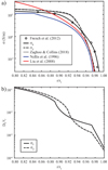Fig. 1 Panela: electrical conductivity profiles in the outer 20% of the radius of Jupiter. The black line shows the parametrization σF(r) of the ab initio simulation data points (black circles) by French et al. (2012). The dotted red line shows theprofile published in Zaghoo & Collins (2018), while the solid red line shows the extension σZ (r) used here. The profiles suggested by Liu et al. (2008) (green) and Nellis et al. (1999) (blue) are shown for comparison. Panel b: magnetic diffusivity scale height Dλ ∕rJ for σF and σZ.

2 Methods and data

2.1 Estimating dynamo action

The ratio of inductive to diffusive effects in the induction equation, 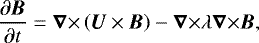$$\frac{\partial B}{\partial t}=\nabla \times \left(U\times B\right)-\nabla \times \lambda \nabla \times B,$$(1)

can be quantified by the magnetic Reynolds number 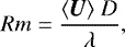$$Rm=\frac{\langle U\rangle D}{\lambda },$$(2)

where λ = 1∕(μσ) is the magnetic diffusivity, with μ the magnetic permeability and σ the electrical conductivity. Angular brackets generally denote rms values at a given radius throughout the paper; thus ⟨U⟩ stands for 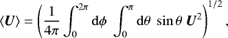$$\langle U\rangle ={\left(\frac{1}{4\pi }{\displaystyle {\int }_0^{2\pi }\text{d}}\varphi {\displaystyle {\int }_0^{\pi }\text{d}}\theta \sin \theta U^2\right)}^{1/2},$$(3)

with θ being the colatitude and ϕ the longitude.

The typical length scale D is hard to estimate, and the planetary radius is often used for simplicity. Since σ decreases steeply in the SDCR, the length scale is determined by the conductivity or magnetic diffusivity scale height: $$D_{\lambda }=\frac{\lambda }{\partial \lambda /\partial r}=-\frac{\sigma }{\partial \sigma /\partial r},$$(4)

and the modified magnetic Reynolds number, $$R{m}^{(1)}=\frac{\langle U\rangle D_{\lambda }}{\lambda }$$(5)

should be used. Since D_λ is small and λ decreases steeply with radius, most of the SDCR of Jupiter is characterized by a small magnetic Reynolds number Rm⁽¹⁾ < 1, and the magnetic field dynamics becomes quasi-stationary (Liu et al. 2008), obeying the simplified induction equation $$\nabla \times \frac{j}{\sigma }\approx \nabla \times (U\times \tilde{B}).$$(6)

Here, j is the current density and $\tilde{B}$ the strong background field produced by the dynamo acting deeper in the planet. The LIF $\widehat{B}$ is given by Ampere’s law: $$j=\nabla \times \widehat{B}/\mu .$$(7)

The steep σ profile dominates the radial dependence of j and $\widehat{B}$ in the SDCR. The current density is thus dominated by the horizontal components, where radial gradients in $\widehat{B}$ contribute (Liu et al. 2008; Wicht et al. 2018): $$j\approx j_H\approx \widehat{r}\times \frac{\partial }{\partial r}{\widehat{B}}_H.$$(8)

Index H denotes the horizontal components; the radial current can be neglected in comparison.

Along the same lines, the horizontal components of Eq. (6) can be approximated by $$\frac{1}{r}\frac{\partial }{\partial r}\frac{r}{\sigma }{j}_H\approx -\widehat{r}\times {[\nabla \times (U\times \tilde{B})]}_H,$$(9)

where $\widehat{r}$ is the radial unit vector. Integration in radius yields the integral current density estimate introduced by Liu et al. (2008), which we identify with an upper index (I): $$j_H^{(I)}=\frac{\sigma }{r}{\left[\frac{r}{\sigma }{j}_H\right]}_{r_J}+\widehat{r}\times \frac{\sigma }{r}{\displaystyle {\int }_r^{r_J}}\text{d}{r}^{\prime }{r}^{\prime }{[\nabla \times (U\times \tilde{B})]}_H.$$(10)

The square brackets with a lower index r_J indicate that the expression should be evaluated at the outer boundary.

For a predominantly zonal flow, we can use the approximation $$\begin{array}{lll}{\left[\nabla \times \left(U\times \tilde{B}\right)\right]}_H\hfill & \approx \hfill & -\frac{{\overline{U}}_{\varphi }}{r\sin \theta }\left(\frac{\partial }{\partial \varphi }{\tilde{B}}_{\theta }\right)\widehat{\theta }\hfill \\ \hfill & \hfill & +\frac{1}{r}\left[\frac{\partial }{\partial r}\left(r{\overline{U}}_{\varphi }{\tilde{B}}_r\right)+\frac{\partial }{\partial \theta }\left({\overline{U}}_{\varphi }{\tilde{B}}_{\theta }\right)\right]\widehat{\varphi },\hfill \end{array}$$(11)

where ${\overline{U}}_{\varphi }$ is the zonal flow component and $\widehat{\theta }$ and $\widehat{\varphi }$ are unit vectors in latitudinal and azimuthal direction, respectively.

The integral estimates for the two horizontal current components are then given by $$\begin{array}{lll}{j}_{\theta }^{(I)}\hfill & =\hfill & \frac{\sigma }{r}{\left[\frac{r}{\sigma }{j}_{\theta }\right]}_{r_J}-\frac{\sigma }{r}\left({\left[r{\overline{U}}_{\varphi }{\tilde{B}}_r\right]}_{r_J}-{\left[r{\overline{U}}_{\varphi }{\tilde{B}}_r\right]}_r\right)\hfill \\ \hfill & \hfill & -\frac{\sigma }{r}{\displaystyle {\int }_r^{r_J}}\text{d}{r}^{\prime }\frac{\partial }{\partial \theta }({\overline{U}}_{\varphi }{\tilde{B}}_{\theta }),\hfill \end{array}$$(12)

and $$j_{\varphi }^{(I)}=\frac{\sigma }{r}{\left[\frac{r}{\sigma }{j}_{\varphi }\right]}_{r_J}-\frac{\sigma }{r}{\displaystyle {\int }_r^{r_J}}\text{d}{r}^{\prime }\frac{{\overline{U}}_{\varphi }}{\sin \theta }\frac{\partial }{\partial \varphi }{\tilde{B}}_{\theta }.$$(13)

Since the latitudinal length scale of the zonal winds is smaller than the azimuthal length scale of the magnetic field, we expect that the latitudinal component dominates.

The integral estimate requires the knowledge of the surface currents. While the surface currents are certainly very small, the scaled version σ(r)∕σ(r_J) j may remain significant. Liu et al. (2008) argue that neglecting the surface contribution at least provides a lower bound for the rms current density.

Wicht et al. (2019) confirm that the dynamics indeed becomes quasi-stationary in the SDCR of their Jupiter-like dynamo simulations and that j_θ is indeed the dominant current component where Rm⁽¹⁾ < 1. They also report that the simplified Ohm’s law for a fast-moving conductor, $$j^{(O)}=\sigma (U\times \tilde{B}),$$(14)

provides a significantly better estimate than j^(I). We identify the respective current estimate with an upper index (O). The general Ohm law, $$j=\sigma \left(U\times B+E\right),$$(15)

also contains currents driven by the electric field, which reduces to E = −∇Φ in the quasi-stationary case, where Φ is the electric potential. In the SDCR of Jupiter, this contribution likely proves secondary because the potential differences remain small compared to the induction by fast zonal winds (Wicht et al. 2019).

As the electrical conductivity decreases in the SDCR, the magnetic field approaches a potential field with its characteristic radial dependence. We use this dependence to approximate the background field with $${\tilde{B}}_{\mathcal{l}}(r,\theta ,\varphi )\approx {\left(\frac{r_J}{r}\right)}^{\mathcal{l}+2}{B}_{\mathcal{l}}(r_J,\theta ,\varphi ),$$(16)

where the index ℓ denotes themagnetic field contribution at spherical harmonic degree ℓ. This provides a suitable approximation as long as the LIF remains a small contribution of the total field (Wicht et al. 2019).

Given a surface field model and an electrical conductivity profile, Ohm’s law for a fast moving conductor and a predominantly zonal flow suggests $$j\approx j_{\theta }^{(O)}\widehat{\theta }=\sigma {\overline{U}}_{\varphi }{\tilde{B}}_r\widehat{\theta }.$$(17)

When using this result to constrain the outer-boundary currents, the alternative integral estimates, Eqs. (12) and (13), yield $$j_{\theta }^{(I)}=\sigma {\overline{U}}_{\varphi }{\tilde{B}}_r-\frac{\sigma }{r}{\displaystyle {\int }_r^{r_J}}\text{d}{r}^{\prime }\frac{\partial }{\partial \theta }({\overline{U}}_{\varphi }{\tilde{B}}_{\theta })$$(18)

and $$j_{\varphi }^{(I)}=-\frac{\sigma }{r}{\displaystyle {\int }_r^{r_J}}\text{d}{r}^{\prime }\frac{{\overline{U}}_{\varphi }}{\sin \theta }\frac{\partial }{\partial \varphi }{\tilde{B}}_{\theta },$$(19)

respectively. A comparison of the estimates shows that j^(I) and j^(O) will remain very similar at shallow depths. When the flow decays very deeply with depth however, the integral contributions in Eqs. (18) and (19) dominate below some radius and cause larger deviations, as we show below.

Calculating the LIF requires to uncurl Ampere’s law, which reduces to integrating Eq. (8) in the SDCR of Jupiter. When using j^(O), this yields $${\widehat{B}}_H\approx {\displaystyle {\int }_r^{r_J}}\text{d}{r}^{\prime }\frac{\widehat{r}\times (U\times \tilde{B})}{\lambda }.$$(20)

Since the electrical conductivity profile rules the radial dependence, the integral can be approximated by $${\widehat{B}}_H\approx \frac{D_{\lambda }}{\lambda }\widehat{r}\times (U\times \tilde{B}).$$(21)

We assume here that the LIF vanishes at the outer boundary. For a dominantly azimuthal flow, the primary LIF component is also azimuthal: $${\widehat{B}}_{\varphi }\approx \frac{D_{\lambda }}{\lambda }{\overline{U}}_{\varphi }{\tilde{B}}_r.$$(22)

This suggests that the rms value scales with Rm⁽¹⁾, $$\langle {\widehat{B}}_H\rangle \approx R{m}^{(1)}\langle \tilde{B}\rangle ,$$(23)

assuming that the correlation between ${\overline{U}}_{\varphi }$ and ${\tilde{B}}_r$ is of little relevance.

The radial LIF can be estimated based on the radial component on the quasi-stationary induction Eq. (1): $$\lambda {\nabla }^2{\widehat{B}}_r\approx -\widehat{r}\cdot \nabla \times (U\times \tilde{B}).$$(24)

When approximating Ohmic dissipation by $\lambda {\widehat{B}}_r/D_{\lambda }^2$, this yields: $${\widehat{B}}_r\approx -\frac{D_{\lambda }^2}{\lambda }\widehat{r}\cdot \nabla \times (U\times \tilde{B}),$$(25)

which reduces to $${\widehat{B}}_r\approx -\frac{D_{\lambda }^2}{\lambda }\frac{{\overline{U}}_{\varphi }}{r\sin \theta }\frac{\partial }{\partial \varphi }{\tilde{B}}_r$$(26)

for a predominantly zonal flow. This suggest that the rms radial LIF should roughly scale with the second modified magnetic Reynolds number $$R{m}^{(2)}=\frac{\langle U\rangle D_{\lambda }^2}{\lambda D}$$(27)

like $$\langle {\widehat{B}}_r\rangle \approx R{m}^{(2)}\frac{D}{D_{\varphi }}\langle \tilde{B}\rangle .$$(28)

Here, D_ϕ is the azimuthal length scale of the background field. Since D_λ ≪ D_ϕ, the radial LIF is much smaller than its horizontal counterpart (Wicht et al. 2019).

2.2 Data

The electric current and LIF estimates discussed above require a conductivity profile, a zonal flow model, and a surface magnetic field model. For the heating and entropy estimates that we derived in Sect. 3, we also need density, temperature, and thermal conductivity profiles. We adopt the interior model calculated by Nettelmann et al. (2012) and French et al. (2012), which is the only one that provides all the required information. We note however that recent Juno gravity data suggest that the interior of Jupiter may be more complex than anticipated in this model (Debras & Chabrier 2019).

Ab initio simulations of the electrical conductivity by French et al. (2012) provide 12 data points at different depths. Figure 1 shows the values in the outer 20% of the radius of Jupiter and the parametrization σ_F(r) developed for our analysis. A linear branch, $${\sigma }_F(r)={\sigma }_r+({\sigma }_m-{\sigma }_r)\frac{r-r_r}{r_m-r_r},$$(29)

covers the smoother inner part r < r_m. An exponential branch, $${\sigma }_F(r)={\sigma }_m\exp \left(\left[\frac{r-r_m}{r_m-r_r}+b{\left(\frac{r-r_m}{r_m-r_r}\right)}^2\right]\frac{{\sigma }_m-{\sigma }_r}{{\sigma }_m}\right),$$(30)

describes the steeper decay for r_m < r < r_e with b = 7.2. Matching radius r_m = 0.89 r_J and reference radius r_r = 0.77 r_J are chosen where ab initio data points have been provided.

A double-exponential branch, $${\sigma }_F(r)={\sigma }_e\exp \left(d\left[\exp \left(c\frac{r-r_e}{r_m-r_r}\right)-1\right]\right),$$(31)

is required to capture the super-exponential decrease for r ≥ r_e = 0.972 r_J. The additional free parameter is c = 10, while σ_e = σ(r_e) and $$d=\frac{1}{c}\left(1+2b\frac{r_e-r_m}{r_m-r_i}\right)\frac{{\sigma }_m-{\sigma }_r}{{\sigma }_m}.$$(32)

The dotted red line in panel a of Fig. 1 shows the conductivity model used to study dynamo action in Jupiter and Jupiter-like exoplanets by Zaghoo & Collins (2018). This is based on measurements which suggest a higher electrical conductivity in the metallic hydrogen phase than previous data. Unfortunately, Zaghoo & Collins (2018) do not discuss how the results were extrapolated to Jovian conditions. The solid red line in Fig. 1 shows the respective parametrization σ_Z (r) used for our analysis, which retraces the published curve and connects to previously published parametrizations (green and blue) at lower densities (Nellis et al. 1996; Liu et al. 2008). We note however that these parametrizations are based on data (Weir et al. 1996) which may have been attributed to overly low temperatures according to a recent analysis by Knudson et al. (2018).

Though model σ_Z(r) is somewhat arbitrary, it serves to illustrate the impact of conductivity uncertainties in our study. Close to r_J where conductivities remain insignificant, σ_F is many orders of magnitude larger than σ_Z. The ratio σ_F∕σ_Z decreases with depth, reaching 10² around 0.97 r_J and 10 around 0.96 r_J. The two models finally cross at about 0.95 r_J. At about 0.925 r_J, the ratio reaches a minimum of 0.05 and then slowly increases with depth to 0.35 at 0.8 r_J. Table 1 list values of both conductivity models for selected radii.

Panel b of Fig. 1 and selected values listed in Table 1 demonstrate that the magnetic diffusivity scale heights D_λ differ much less than the conductivities themselves. Electric currents, LIFs, and Ohmic heating depend linearly on σ but on different powers of D_λ. The differences between the results for the two conductivity models is therefore predominantly determined by σ and can easily be scaled from one to the other.

The three different zonal flow models explored here are illustrated in Fig. 2. Table 1 lists rms values $\langle {\overline{U}}_{\varphi }\rangle$ at selected radii. All reproduce the observedzonal winds at r = r_J (Porco et al. 2003; Vasavada & Showman 2005). We use a running average of the surface profile with a window width of one degree and represent the result with 256 (nearly) evenly spaced latitudinal grid points for our calculations.

The three flow models differ at depth. The most simple one, U_G, assumes geostrophy in each hemisphere, that is, the flow depends only on the distance s = rsinθ to the rotation axis. Kaspi et al. (2018) describe the depth decay of the equatorially antisymmetric zonal flow with profiles constrained by the Juno gravity measurements. We apply their “latitude-independent” model version to the total zonal flow and refer to this model as U_K. The rms amplitude of U_K has decreased by one order of magnitude at about 0.95 r_J and by two orders of magnitude around 0.925 r_J.

We also consider the “deep” model suggested by Kong et al. (2018), who assume an exponential depth decay and an additional linear dependence on the distance z = cosθ to the equatorial plane. Like for U_K, our respective model U_Z assumes that the depth and z dependences, which were originally derived for the equatorially antisymmetric contributions, apply to the whole flow. The rms velocity in U_Z decays more smoothly with depth than in U_K, having decreased by one order of magnitude at about 0.935 r_J and by two orders of magnitude at about 0.905 r_J.

Figure 2 shows that U_G and U_K have discontinuities at the equatorial plane. These pose a problem when calculating the latitudinal zonal flow derivatives required for the integral estimate $j_{\theta }^{(I)}$ (see Eq. (18)). Formally, the derivative becomes infinite at the equator. Practically however, the impact of the discontinuity depends on the model setup and on the methods used for calculating the derivatives. We tested the impact on rms current density estimates by comparing calculations covering all latitudes with counterparts where the derivatives were explicitly set to zero in a six-degree belt around the equator. Simple first-order finite differences with 256 grid points at each radial level are generally used for calculating the derivative. For flow U_Z, which has been constructed to avoid the discontinuity (Kong et al. 2018), the belt contributes not more than one percent to $\langle j_{\theta }^{(I)}\rangle$ at any radius, which is less than the surface fraction it represents. For flow U_K, the contribution is even smaller due to the faster decay of the flow amplitude. However, for U_G the belt contributes 20% to the rms current for radii below 0.94 r_J, which is a clear sign that the unphysical discontinuity causes problems. We take a conservative approach and only consider flow model U_Z in connection with estimate $j_{\theta }^{(I)}$ below.

The radius where Rm⁽¹⁾ = 1, which we refer to as r₁ in the following, roughly marks the point where the approximations discussed above break down (Wicht et al. 2019). Figure 3a illustrates the Rm⁽¹⁾ profiles that result from combining σ_F and σ_Z with rms values for the three zonal flow models. Table 1 compares values at some selected radii. These modified magnetic Reynolds numbers exceed unity between r₁ = 0.957 r_J for the combination σ_Z and U_K and r₁ = 0.967 r_J for σ_F and U_G. All r₁ values are listed in Table 2.

Green lines in Fig. 3 show Rm⁽¹⁾ profiles for a typical convective velocity of 10 cm s⁻¹ suggested by scaling laws (e.g., see Duarte et al. 2018). Numerical simulations show that the velocity increases with radius, an effect not taken into account here. The comparison of the different Rm⁽¹⁾ profiles suggests that zonal-flow-related dynamo action should dominate at least in the outer 9% in radius.

For the surface magnetic field of Jupiter we use the JRM09 model by Connerney et al. (2018), which provides information up to spherical harmonic degree ℓ = 10. The more recent model by Moore et al. (2018) is only slightly different. In order to check the impact of smaller-scale contributions, we also tested the numerical model G14 by Gastine et al. (2014), which reproduces the large-scale field of Jupiter and provides harmonics up to ℓ = 426. Since it turned out that the impact of the smaller scales is very marginal, the results are not shown here.

3 Dissipative heating and entropy production in Jupiter

Liu et al. (2008) constrain the depth of the zonal winds by assuming that the related total Ohmic heating should not exceed the heat flux out of the planet. Unfortunately, this assumption is incorrect, as we show in the following. In order to arrive at more meaningful constraints, we start by reviewing some fundamental considerations.

In a quasi-stationary state, where flow and magnetic field are maintained by buoyancy and induction against dissipative losses, the conservation of energy simply states that the heat flux Q_o = Q(r_o) through the outer boundary is the sum of the flux Q_i = Q(r_i) through the inner boundary and the total internal heating H: $$Q_{\text{o}}=Q_{\text{i}}+H.$$(33)

We note that neither viscous nor Ohmic heating contribute to H. Since flow and magnetic field are maintained by the heat flux through the system, they cannot be counted as net heat sources (Hewitt et al. 1975; Braginsky & Roberts 1995).

When furthermore neglecting the effects of helium segregation, core erosion, and planetary shrinking as potential energy sources, the only remaining contribution is the slow secular cooling of the planet. The volumetric heat source is then given by $$h=\tilde{\rho }\tilde{T}\frac{\partial \tilde{S}}{\partial t},$$(34)

where the tilde indicates the hydrostatic, adiabatic background state (Braginsky & Roberts 1995). Assuming that convection maintains an adiabat at all times, $\partial \tilde{S}/\partial t$ remains homogeneous throughout the convective region and obeys (Jones 2014) $$\frac{\partial \tilde{S}}{\partial t}=\left(Q_{\text{o}}-Q_{\text{i}}\right)/{\displaystyle {\int }_V\text{d}}V\tilde{\rho }\tilde{T},$$(35)

where ∫_VdV denotes an integration over the whole convective volume. We note however that the thermal evolution could be more complex should Jupiter indeed harbor stably stratified regions.

In order to assess dissipative heating, one must consider the local heat equation $$\tilde{\rho }\tilde{T}\left(\frac{\partial s}{\partial t}+U\cdot \nabla s\right)=\nabla \cdot \left(k\nabla T\right)+h+\phi ,$$(36)

where φ denotes the volumetric dissipative heat source and k the thermal conductivity. When assuming a steady state and adopting the anelastic approximation $\nabla \cdot (\tilde{\rho }U)=0$, the integration over the shell between the inner boundary r_i and radius r yields $$Q_D(r)+Q_A(r)=Q_i+{\displaystyle {\int }_{r_i}^r\text{d}}{r}^{\prime }{\displaystyle {\int }_F\text{d}}F\left(h+\phi +\tilde{\rho }s{U}_r\frac{\partial \tilde{T}}{\partial r}\right).$$(37)

The left-hand side is the total flux through the boundary at r, that is, the sum of the diffusive contribution, $$Q_D(r)=-{\displaystyle {\int }_F\text{d}}Fk\frac{\partial T}{\partial r},$$(38)

and the advective contribution, $$Q_A(r)={\displaystyle {\int }_{F(r)}\text{d}}F\tilde{\rho }\tilde{T}s{U}_r.$$(39)

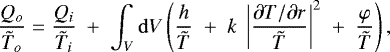
The right-hand side of Eq. (37) reflects the influx through the lower boundary Q_i plus three volumetric contributions: the slow secular cooling, the dissipative heating, and the adiabatic cooling. Writing the adiabatic cooling in terms of Q_A yields the relation $$\begin{array}{lll}{Q}_D(r)+Q_A(r)\hfill & =\hfill & Q_i+{\displaystyle {\int }_{r_i}^r\text{d}}{r}^{\prime }{\displaystyle {\int }_F\text{d}}F\left(h+\phi \right)\hfill \\ \hfill & \hfill & -{\displaystyle {\int }_{r_i}^r\text{d}}{r}^{\prime }{Q}_A(r^{\prime })/D_T(r^{\prime }),\hfill \end{array}$$(40)

where $D_T=-\tilde{T}/(\partial \tilde{T}/\partial r)$, which is the thermal scale height.

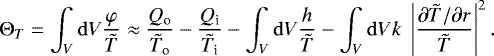
Integrating Eq. (40) over the whole convective volume and using Eq. (33) reveals that the total dissipative heating Φ_T is balanced by the total adiabatic cooling: $${\Phi }_T={\displaystyle {\int }_V\text{d}}V\phi ={\displaystyle {\int }_{r_i}^{r_o}\text{d}}{r}^{\prime }{Q}_A(r^{\prime })/D_T(r^{\prime }).$$(41)

The total adiabatic cooling is actually identical to the buoyancy power P that drives convection and thus the dynamo mechanism. Multiplying the buoyancy term in the Navier–Stokes equation with velocity and integrating over the convective volume to yield the total convective power input indeed gives the same expression (Braginsky & Roberts 1995). Equation (41) therefore simply states that dissipation is balanced by the power input P to the system, a fact used in many scaling laws to establish how the rms magnetic field strength or the rms velocity scale with P (Christensen & Aubert 2006; Christensen et al. 2009; Davidson 2013; Yadav et al. 2013).

Equation (41) requires knowledge of Q_A at each radius. Since Q_A itself depends on the distribution of dissipative heat sources however, an additional condition is required. Assuming that Ohmic heating and adiabatic cooling not only cancel globally but, at least roughly, also at each radius offers a simple solution used in most scaling laws (though never stated explicitly). With the exception of thin thermal boundary layers, the heat flux is then dominated by the advective contribution, so that $$Q_A(r)\approx Q_i+{\displaystyle {\int }_{r_i}^r\text{d}}r{\displaystyle {\int }_F\text{d}}Fh.$$(42)

Adopting the interior model by Nettelmann et al. (2012) and French et al. (2012) and the observed flux Q_o = 3.35 × 10¹⁷ W from the interior of the planet (Guillot & Gautier 2015) allows us to calculate h via Eq. (34). Because the inner core occupies only 10% in radius, Q_i can be neglected. When for example assuming that h also describes the cooling of the rocky core, Q_i is two orders of magnitude smaller than Q_o.

Plugging Eq. (42) into Eq. (41) finally allows us to calculate the total dissipative heating: $${\Phi }_T=1.20\times {10}^{18}\text{W}.$$(43)

The result reveals that dissipative heating can in fact exceed the heat flux out of the interior of Jupiter by a factor of 3.6. Gastine et al. (2014) obtained a power estimate that is about 50% smaller than this latter figure because they used a simplified formula provided by Christensen et al. (2009).

Considering the entropy rather than the heat balance avoids the need to come up with an additional condition (Hewitt et al. 1975; Gubbins et al. 1979, 2003; Braginsky & Roberts 1995). Dividing the heat equation Eq. (36) by temperature and integrating over the convective volume yields the entropy budget: $$\frac{Q_o}{{\tilde{T}}_o}=\frac{Q_i}{{\tilde{T}}_i}+{\displaystyle {\int }_V\text{d}}V\left(\frac{h}{\tilde{T}}+k{\left|\frac{\partial T/\partial r}{\tilde{T}}\right|}^2+\frac{\phi }{\tilde{T}}\right),$$(44)

where we have once more used the anelastic approximation $\nabla \cdot (\tilde{\rho }U)=0$. When assuming that the temperature profile stays close to the adiabat, the total dissipative entropy production Θ can thus be approximated by $${\Theta }_T={\displaystyle {\int }_V\text{d}}V\frac{\phi }{\tilde{T}}\approx \frac{Q_{\text{o}}}{{\tilde{T}}_{\text{o}}}-\frac{Q_{\text{i}}}{{\tilde{T}}_{\text{i}}}-{\displaystyle {\int }_V\text{d}}V\frac{h}{\tilde{T}}-{\displaystyle {\int }_V\text{d}}Vk{\left|\frac{\partial \tilde{T}/\partial r}{\tilde{T}}\right|}^2.$$(45)

An upper bound for the total dissipative heating can be derived when assuming that ${\tilde{T}}_i$ is the highest temperature in the system (Hewitt et al. 1975; Currie & Browning 2017): $$\Phi <{\tilde{T}}_i{\displaystyle {\int }_V\text{d}}V\frac{\phi }{\tilde{T}}<\frac{{\tilde{T}}_i}{{\tilde{T}}_o}{Q}_{\text{o}}.$$(46)

Using once more the internal model by Nettelmann et al. (2012) puts the upper bound at 10² Q_o for Jupiter, which is at least consistent with estimate (43).

When complementing the internal model with the thermal conductivity profile by French et al. (2012), we can quantify the different terms in the entropy budget of Jupiter (Eq. (45)). Because of the strong temperature contrast between the outer boundary and the deeper convective region, the entropy flux through the outer boundary clearly dominates. The total dissipative entropy production is therefore given by $${\Theta }_T\approx Q_{\text{o}}/{\tilde{T}}_{\text{o}}=2.0\times {10}^{15}\text{W/K}.$$(47)

The second-largest term in Eq. (45), the entropy due to the secular cooling, is already two orders of magnitude smaller, at 3.0 × 10¹³ W/K. The two remaining terms, entropy flux through the inner boundary and the diffusive entropy flux down the adiabat, are only of order 10¹¹ W/K.

Since the magnetic diffusivity is about 10⁶ times larger than its viscous counterpart in planetary dynamo regions, Ohmic heating is by far the dominating factor. We can use the current density estimates to predict the Ohmic heating due to the zonal flows above radius r: $${\Phi }_O(r)={\displaystyle {\int }_r^{r_J}}\text{d}{r}^{\prime }{\displaystyle {\int }_F\text{d}}F\frac{j^2}{\sigma }.$$(48)

The conditions $${\Phi }_O(r)\le {\Phi }_T=1.20\times {10}^{18}\text{W}$$(49)

provides a possible constraint for the depth of the zonal winds in Jupiter.

The dissipative entropy production related to the Ohmic heating is given by $${\Theta }_O(r)\approx {\displaystyle {\int }_r^{r_J}}\text{d}{r}^{\prime }{\displaystyle {\int }_F\text{d}}F\frac{j^2}{\sigma \tilde{T}}.$$(50)

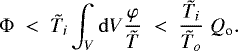
This can be used for the alternative depth constraint $${\Theta }_O(r)\le {\Theta }_T=2.0\times {10}^{15}\text{W/K}.$$(51)

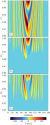Fig. 2 Zonal flow models used in this study. Prograde flows are shown in red and yellow, while blue indicates retrograde directions.

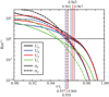Fig. 3 Modified magnetic Reynolds numbers for the three zonal flow and the two conductivity models explored here. Vertical lines mark the radii r1 where Rm(1) = 1. Green lines show profiles for a typical convective velocity of 10 cm s−1 suggested by scaling laws.

4 Dynamo action in the SDCR of Jupiter

In the following we apply the methods developed above to the SDCR of Jupiter. We first estimate the electric currents and induced fields in Sect. 4.1 and then explore whether Ohmic heating or entropy can serve to constrain the depth of the zonal winds in Sect. 4.2.

4.1 Electric currents and locally induced field

We start by discussing the current estimates for the different zonal flow and conductivity model combinations. Figure 4a compares rms values of integral estimates j^(I) and Ohm’s law estimates j^(O) for conductivity model σ_F and flow U_Z. The integral estimates of the latitudinal currents are at least 40 times larger than their azimuthal counterparts for all conductivity and flow model combinations. When using j^(O) as outer boundary condition for j^(I) (blue line in Fig. 4), both estimates remain very similar down to about 0.98 r_J. At 0.97 r_J however, j^(I) is already about 50% larger than j^(O), and at 0.96 r_J the difference has increased to about 250%. When assuming a vanishing outer boundary current for j^(I), the differences are even larger: j^(I) (green line) is 3.5 times larger than j^(O) at 0.97 r_J and about 6 times larger at 0.96 r_J.

Estimates of the rms horizontal and radial LIF are shown in Fig. 4b, based on j^(O) and Eq. (20) for the horizontal and on Eq. (26) for the radial components. The radial LIF is between two and three orders of magnitude smaller than its horizontal counterpart. The rougher estimates (Eqs. (23) and (28)), based on Rm⁽¹⁾ and Rm⁽²⁾, respectively, provide values that are less than a factor two smaller and can thus safely be used for order-of-magnitude assessments; they correctly predict that the rms azimuthal LIF reaches the level of the background field at r₁ and also that the ratio of radial to azimuthal LIF is about Rm⁽²⁾∕Rm⁽¹⁾ = D_λ∕r_J. At r₁, the rms radial LIF is thus roughly three orders of magnitude smaller than the background field or the horizontal LIF. Table 2 lists the relative rms radial LIF (Col. 7) at r₁ (Col. 3) for all σ and flow combinations when using j^(O).

Wicht et al. (2019) demonstrate that the estimates based on Ohm’s-law not only provide good rms but also good local values for their Jupiter-like dynamo simulations. Figure 5 shows the radial surface field of JRM09 in panel a and the radial LIF for σ_F and U_Z at r₁ in panel b. A very distinct pattern of localized field patches can be found where the fast zonal jets around the equator interact with the strong blue patch in the JRM09 model.

The zonal flow pattern remains recognizable in the LIF, as is clearly demonstrated in Fig. 6, which compares zonal flow profiles in panel a with the azimuthal rms of the radial LIF in panel b. Due to the flow geometry, the currents and LIF show a depth-dependent phase shift relative to the surface jets. The equatorial jet, which is so prominent at the surface, contributes very little to dynamo action, since it does not reach down to depths where the electrical conductivity is more significant.

Figure 7 compares spherical harmonic power spectra of the background radial field and the radial LIF. As already apparent from the map shown in Fig. 5, the LIF is dominated by smaller-scale contributions. The spherical harmonic degree spectrum results from the convolution of the complex latitudinal zonal flow structure with the background field. At r₁, the dipole contribution in the LIF isabout 10⁻⁴ times smaller than the respective background field contribution. For degree ℓ = 10, the ratio has increased to 10⁻². The spectrum peaks at ℓ = 12 but has alsosignificant contributions from even higher degrees.

The spherical harmonic order spectrum, shown in panel b of Fig. 7, is very different. The action of the axisymmetric zonal flow on ${\tilde{B}}_r$ excites no additional harmonic orders so that the spectrum remains confined to m ≤ 10. The LIF spectrum is rather flat but has no axisymmetric contribution. At m = 10, the rms LIF amplitude reaches roughly 25% of the background field.

The results for the conductivity model σ_F presented so far can roughly be scaled to model σ_Z by multiplying with the conductivity ratio σ_Z∕σ_F. Around 0.97 r_J, the LIF is two orders of magnitude weaker, and the difference decreases with depth, reaching about one order of magnitude around 0.96 r_J. Where Rm⁽¹⁾ = 1, on the other hand, the LIF reaches comparable values for both conductivity models. The different flow models yield very similar LIF patterns, albeit with the different amplitudes indicated in Fig. 4.

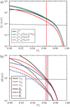Fig. 4 Panel a: rms current density estimates for flow model UZ and conductivity model σF. Panel b: estimates of rms radial and horizontal LIF. The profile of $\langle {\tilde{B}}_r\rangle$ has been included for comparison. Vertical lines mark the radii where Rm(1) = 1 for the different flow models. Current density estimates j(O) and conductivity model σF have been used.

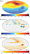Fig. 5 Maps of panel a: radial surface field in the Jupiter field model JRM09, panel b: radial LIF at r1 = 0.965 rJ, and panel c: local Ohmic heating $q={\int }_r^{r_{\text{J}}}\text{d}r{j}^2/\sigma$ at r = r1 = 0.965 rJ. Flow model UZ, conductivityσF, and current density estimates j(O) (for panel c) have been used. Outward (inward) directed field is shown in red (blue).

4.2 Ohmic heating and entropy constraint

We now use the electric current estimates to calculate Ohmic heating and entropy production. Panel c of Fig. 5 shows the map of Ohmic heat flux density 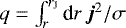$q={\displaystyle {\int }_r^{r_{\text{J}}}\text{d}}r{j}^2/\sigma$ at radius r₁ when using j^(O), σ_F, and U_Z. The currents induced by interaction between the fierce zonal jets close to the equator and the strong blue patch in JRM09 not only yield a highly localized LIF but also intense local heating. While the action of various other zonal jets reaches a lower level, the related pattern remains roughly recognizable in the form of thin heating bands. The azimuthal mean of q shown in panel c of Fig. 6 clearly illustrates the correlation between heating and the zonal jets. Like for the LIF, there is a depth-dependent phase shift between the observed surface zonal wind profile and the Ohmic heating pattern.

Panel a of Fig. 8 compares the Ohmic heating profiles Φ_O (r) for the different zonal flow and electrical conductivity models. Because of the extremely low conductivity, heating remains negligible in the outer two percent in radius. When using j^(O), the outermost radius where Φ_O reaches the level of Φ_T is r_Φ = 0.950 r_J for flow U_G and both conductivity models. When using U_K and σ_F, the Ohmic heating always remains below Φ_T. Results based on j^(I) (not shown) are less sensitive to the differences between the three flow models at depth and are generally similar to the results for U_G and j^(O).

The different r_Φ values where Φ_O = Φ_T have been marked by vertical lines in Fig. 8 and are listed in Col. 5 of Table 2. All are located below the radii r₁ where Rm⁽¹⁾ = 1 for the respective model combinations (Col. 3) and thus in a region where the approximations employed here break down. The maximum Ohmic heating reached at r₁ remains nearly one order of magnitude below Φ_T (see Col. 8 of Table 2).

Similar inferences hold for the entropy production shown in panel b of Fig. 8. The entropy condition is less strict than the power-based heat condition, and the radii r_Θ where the different models exceed the threshold Θ_T (Col. 6 of Table 2) are somewhat deeper than respective r_Φ values. The largest value of r_Θ = 0.955 is found for the combination U_G and σ_Z. The combinationof U_K and σ_F, on the other hand, yields the deepest value of r_Θ = 0.929.

The exploration of numerical dynamo simulations by Wicht et al. (2019) suggest that j^(O) may provide an acceptable estimate for a limited region below r₁, at least down to where Rm⁽¹⁾ = 5. Column 4 of Table 2 demonstrates that even the radius r₁₀ where Rm⁽¹⁾ = 10 lies deeper than r_Φ for most flow and conductivity combinations. The only exceptions are the results for the geostrophic flow. This could indicated that strictly geostrophic flows would indeed violate the heating contraint.

Fig. 6 Panel a: UZ profiles at different depths; the grey background color highlights where surface jets are prograde. Panel b: azimuthal rms radial LIF and panel c: heat flux $q={\int }_r^{r_{\text{J}}}\text{d}r{j}^2/\sigma$ at three different depths. Conductivity model σF, flow UZ, and estimatej(O) have been used.

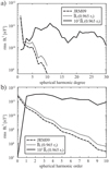Fig. 7 Power spectra of rms radial field contributions (Mauersberger-Lowes) for JRM09, the downward continued ${\tilde{B}}_r$ and the radial LIF ${\widehat{B}}_r$ at r1 = 0.965 rJ: panel a: spherical harmonic degree spectrum; panel b: harmonic order spectrum. The LIF has been amplified by 1000. Flow UZ and conductivity σF have been used.

5 Discussion and conclusion

The dominance of Ohmic dissipation in the outer few percent of the radius of Jupiter leads to simple quasi-stationary dynamo action. This can be exploited for estimating the electric currents and the LIFs with surprisingly high quality (Wicht et al. 2019), once a conductivity profile, a surface magnetic field model, and flow model are given. Here we explored two conductivity profiles, used the new Juno-based JRM09 field model, and tested two zonal flow models suggested from inversions of Juno gravity measurements. A geostrophic zonal flow model was also considered as a third option.

The estimates roughly apply to the upper four percent in radius, or roughly 3000 km, where the modified magnetic Reynolds number Rm⁽¹⁾ is smaller than one. The radial LIF in this quasi-stationary dynamo region typically reaches rms values in the order of μT with peak values up to 15 μT. Could such a small contribution be measured by the Juno magnetometer? The instrument has been designed to provide a nominal vector accuracy of 1 in 10⁴. Since the surface field reaches peak values of about 2 mT, the LIF could indeed be detectable.

One would still have to separate the LIF from contributions produced deeper in the planet. What should help with this task is the distinct pattern imprinted by the zonal flows, which also leads to a distinct magnetic spectrum. The LIF spectrum peaks at degree ℓ = 12 and has significant contributions at even higher degrees. At ℓ = 10, the largest degree provided by JRM09, the LIF amounts to about 1% of the background field, which seems smaller than the estimated JRM09 precision (Connerney et al. 2018). Updated future models, based on a larger number of Juno orbits, will provide smaller-scale details and increase the chances of identifying the LIF. Another possibility is a dedicated analysis of measurements around the “big blue spot” in JRM09, where induction effects are particularly strong.

Our analysis of the heat balance of Jupiter shows that Ohmic heating can significantly exceed the heat flux Q_o out of the interior of the planet. Using the interior model by Nettelmann et al. (2012) and French et al. (2012) suggests a total dissipative heating of Φ_T = 3.58 Q_o = 1.20 × 10¹⁸ W.

It would be interesting to repeat this assessment for the newer Jupiter models that include stably stratified regions (Debras & Chabrier 2019). However, the most important constraint is the knowledge of Q_o, and the somewhat different distribution of internal heat sources implied by the newer models can only have a limited effect.

While the total Ohmic heating remains typically one order of magnitude below Φ_T, we find extreme lateral variations. Peak values in the Ohmic heating density reach 25 W m⁻² around the “blue spot” in the JRM09, which is nearly five times larger than the mean heat flux density from the interior of Jupiter. These peak values are reached at the bottom of the quasi-stationary region, that is, at a depth of 3000 km. This is much deeper than any (current) remote instrument could reach. For example MWR, the micro-wave instrument on Juno, hopes to detect temperature radiation from up to 1 kbar, which corresponds to a depth of about 600 km. However, the local heating may trigger convective plumes that rise to shallower depths and thus become detectable.

We also estimated the entropy flux out of the interior of Jupiter to 2.0 × 10¹⁵ W K⁻¹. The entropyproduced by zonal-wind-related Ohmic heating in the quasi-stationary region does not exceed this value for any model combination. This means that neither Ohmic heating nor the entropy production offer any reliable constraint on the depth of the zonal winds.

Below the quasi-stationary region, electric fields become a significant contribution to Ohm’s law, tend to oppose induction effects, and lead to weaker electric currents than predicted by our approximations. Wicht et al. (2019) demonstrate that the currents remain roughly constant below the depth where Rm⁽¹⁾ ≈ 5 in their numerical simulations. However, this may be different in Jupiter where the magnetic Reynolds numbers reach values orders of magnitude higher than in their computer models.

Figure 3 demonstrates that Rm⁽¹⁾ increases to a value of at least 10³ at 0.90 r_J. This is a consequence of the electrical conductivity profiles that easily overcompensate the depth-decrease in zonal flow velocities indicated by Juno gravity measurements. The zonal flows may therefore actually play a larger role for dynamo action below the quasi-stationary region. While the gravity data convincingly show that the zonal winds must be significantly weaker below about 0.96 r_J, they cannot uniquely constrain their structure or amplitude at this depth.

It has been speculated that the fast observed zonal winds may remain confined to a thin weather layer, where differential solar heating and also moist convection could significantly contribute to the dynamics (see e.g., Showman 2007 or Thomson & McIntyre 2016). Kong et al. (2018) show that the gravity signal can then be explained by an independent zonal flow system that reaches down to about 0.7 r_J with typical amplitudes of about 1 m s⁻¹ and that has larger latitudinal scales than the surface winds. The strongest local dynamo action happens towards the bottom of the quasi-stationary region where models U_K and U_Z reach velocities of about 10 m s^-1. The currents and magnetic fields induced by this alternative flow model should therefore be roughly an order of magnitude weaker than for U_K or U_Z. Consequently, Ohmic heating and entropy production would be two orders of magnitude lower and play practically no role for the global power or entropy budgets.

Below 0.96 r_J, full 3D numerical simulations would be required to model the zonal-wind-related dynamo action. However, since they cannot be run at altogether realistic parameters and generally yield a much simpler zonal wind pattern, the results must be interpreted with care (Gastine et al. 2014; Jones 2014; Duarte et al. 2018; Dietrich & Jones 2018). These simulations suggest that even the weaker zonal winds at depth would significantly shear the large-scale field produced by the deeper primary dynamo action. The resulting strong longitudinal (toroidal) flux bundles are converted into observable radial field by the small-scale convective flows present in this region. The combined action of primary and secondary dynamo typically yields a radial surface field that is characterized by longitudinal banded structures and large-scale patches with wavenumber one or two, resulting in a morphology that is often reminiscent of the recent Juno-based field model JRM09 (Gastine et al. 2014; Duarte et al. 2018; Dietrich & Jones 2018).

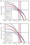Fig. 8 Profiles of panel a: Ohmic heating and panel b: entropy production in the layer above radius r for current estimate j(O). In (a) the solid horizontal line shows the total convective power of 1.2 × 1018 W, while the dotted horizontal line shows the heat flow of Qo = 3.35 × 1017 W from the interior of Jupiter. In (b) the horizontal line indicates the total dissipative entropy production predicted by the entropy flux ΘT = Qo∕To = 2.0 × 1015 W/K through the outer boundary. Vertical lines mark the radii r1 where Rm(1) = 1 (see Fig. 3).

Acknowledgements

This work was supported by the German Research Foundation (DFG) in the framework of the special priority programs “PlanetMag” (SPP 1488) and “Exploring the Diversity of Extrasolar Planets” (SPP 1992).

References

All Tables

All Figures

Fig. 1 Panela: electrical conductivity profiles in the outer 20% of the radius of Jupiter. The black line shows the parametrization σF(r) of the ab initio simulation data points (black circles) by French et al. (2012). The dotted red line shows theprofile published in Zaghoo & Collins (2018), while the solid red line shows the extension σZ (r) used here. The profiles suggested by Liu et al. (2008) (green) and Nellis et al. (1999) (blue) are shown for comparison. Panel b: magnetic diffusivity scale height Dλ ∕rJ for σF and σZ.

In the text

	Fig. 2 Zonal flow models used in this study. Prograde flows are shown in red and yellow, while blue indicates retrograde directions.
In the text

	Fig. 3 Modified magnetic Reynolds numbers for the three zonal flow and the two conductivity models explored here. Vertical lines mark the radii r1 where Rm(1) = 1. Green lines show profiles for a typical convective velocity of 10 cm s−1 suggested by scaling laws.
In the text

	Fig. 4 Panel a: rms current density estimates for flow model UZ and conductivity model σF. Panel b: estimates of rms radial and horizontal LIF. The profile of $\langle {\tilde{B}}_r\rangle$ has been included for comparison. Vertical lines mark the radii where Rm(1) = 1 for the different flow models. Current density estimates j(O) and conductivity model σF have been used.
In the text

	Fig. 5 Maps of panel a: radial surface field in the Jupiter field model JRM09, panel b: radial LIF at r1 = 0.965 rJ, and panel c: local Ohmic heating $q={\int }_r^{r_{\text{J}}}\text{d}r{j}^2/\sigma$ at r = r1 = 0.965 rJ. Flow model UZ, conductivityσF, and current density estimates j(O) (for panel c) have been used. Outward (inward) directed field is shown in red (blue).
In the text

	Fig. 6 Panel a: UZ profiles at different depths; the grey background color highlights where surface jets are prograde. Panel b: azimuthal rms radial LIF and panel c: heat flux $q={\int }_r^{r_{\text{J}}}\text{d}r{j}^2/\sigma$ at three different depths. Conductivity model σF, flow UZ, and estimatej(O) have been used.
In the text

	Fig. 7 Power spectra of rms radial field contributions (Mauersberger-Lowes) for JRM09, the downward continued ${\tilde{B}}_r$ and the radial LIF ${\widehat{B}}_r$ at r1 = 0.965 rJ: panel a: spherical harmonic degree spectrum; panel b: harmonic order spectrum. The LIF has been amplified by 1000. Flow UZ and conductivity σF have been used.
In the text

Fig. 8 Profiles of panel a: Ohmic heating and panel b: entropy production in the layer above radius r for current estimate j(O). In (a) the solid horizontal line shows the total convective power of 1.2 × 1018 W, while the dotted horizontal line shows the heat flow of Qo = 3.35 × 1017 W from the interior of Jupiter. In (b) the horizontal line indicates the total dissipative entropy production predicted by the entropy flux ΘT = Qo∕To = 2.0 × 1015 W/K through the outer boundary. Vertical lines mark the radii r1 where Rm(1) = 1 (see Fig. 3).

In the text

References

- Braginsky, S., & Roberts, P. 1995, Geophys. Astrophys. Fluid Dyn., 79, 1 [NASA ADS] [CrossRef] [Google Scholar]
- Cao, H., & Stevenson, D. J. 2017, Icarus, 296, 59 [NASA ADS] [CrossRef] [Google Scholar]
- Christensen, U., & Aubert, J. 2006, Geophys. J. Int., 116, 97 [NASA ADS] [CrossRef] [Google Scholar]
- Christensen, U. R., Holzwarth, V., & Reiners, A. 2009, Nature, 457, 167 [NASA ADS] [CrossRef] [PubMed] [Google Scholar]
- Connerney, J. E. P., Kotsiaros, S., Oliversen, R. J., et al. 2018, Geophys. Res. Lett., 45, 2590 [NASA ADS] [CrossRef] [Google Scholar]
- Currie, L. K., & Browning, M. K. 2017, ApJ, 845, L17 [NASA ADS] [CrossRef] [Google Scholar]
- Davidson, P. A. 2013, Geophys. J. Int., 195, 67 [NASA ADS] [CrossRef] [Google Scholar]
- Debras, F., & Chabrier, G. 2019, ApJ, 872, 100 [NASA ADS] [CrossRef] [Google Scholar]
- Dietrich, W., & Jones, C. A. 2018, Icarus, 305, 15 [NASA ADS] [CrossRef] [Google Scholar]
- Duarte, L. D. V., Wicht, J., & Gastine, T. 2018, Icarus, 299, 206 [NASA ADS] [CrossRef] [Google Scholar]
- French, M., Becker, A., Lorenzen, W., et al. 2012, ApJS, 202, 5 [NASA ADS] [CrossRef] [Google Scholar]
- Galanti, E., Kaspi, Y., Miguel, Y., et al. 2019, Geophys. Res. Lett., 46, 616 [NASA ADS] [CrossRef] [Google Scholar]
- Gastine, T., Wicht, J., Duarte, L. D. V., Heimpel, M., & Becker, A. 2014, Geophys. Res. Lett., 41, 5410 [NASA ADS] [CrossRef] [Google Scholar]
- Gubbins, D., Masters, T. G., & Jacobs, J. A. 1979, Geophys. J., 59, 57 [NASA ADS] [CrossRef] [Google Scholar]
- Gubbins, D., Alfè, D., Masters, G., Price, G., & Gillan, M. 2003, Geophys. J. Int., 155, 609 [NASA ADS] [CrossRef] [Google Scholar]
- Guillot, T., & Gautier, D. 2015, in Treatise on Geophysics, Planets and Moons, 2nd edn, ed. T. Spohn (Amsterdam: Elsevier), 10, 439 [CrossRef] [Google Scholar]
- Guillot, T., Miguel, Y., Militzer, B., et al. 2018, Nature, 555, 227 [NASA ADS] [CrossRef] [PubMed] [Google Scholar]
- Heimpel, M., Gastine, T., & Wicht, J. 2016, Nat. Geosci., 9, 19 [NASA ADS] [CrossRef] [Google Scholar]
- Hewitt, J. M., McKenzie, D. P., & Weiss, N. O. 1975, J. Fluid Mech., 68, 721 [NASA ADS] [CrossRef] [Google Scholar]
- Iess, L., Folkner, W. M., Durante, D., et al. 2018, Nature, 555, 220 [NASA ADS] [CrossRef] [Google Scholar]
- Iess, L., Militzer, B., Kaspi, Y., et al. 2019, Science, 364, aat2965 [NASA ADS] [CrossRef] [Google Scholar]
- Jones, C. A. 2014, Icarus, 241, 148 [NASA ADS] [CrossRef] [Google Scholar]
- Kaspi, Y., Galanti, E., Hubbard, W. B., et al. 2018, Nature, 555, 223 [NASA ADS] [CrossRef] [PubMed] [Google Scholar]
- Knudson, M. D., Desjarlais, M. P., Preising, M., & Redmer, R. 2018, Phys. Rev. B, 98, 174110 [NASA ADS] [CrossRef] [Google Scholar]
- Kong, D., Zhang, K., Schubert, G., & Anderson, J. D. 2018, Proc. Natl. Acad. Sci., 115, 8499 [Google Scholar]
- Liu, J., Goldreich, P. M., & Stevenson, D. J. 2008, Icarus, 196, 653 [NASA ADS] [CrossRef] [Google Scholar]
- Militzer, B., Soubiran, F., Wahl, S. M., & Hubbard, W. 2016, J. Geophys. Res. (Planets), 121, 1552 [Google Scholar]
- Moore, K. M., Yadav, R. K., Kulowski, L., et al. 2018, Nature, 561, 76 [NASA ADS] [CrossRef] [Google Scholar]
- Moore, K. M., Cao, H., Bloxham, J., et al. 2019, Nat. Astron., 3, 730 [NASA ADS] [CrossRef] [Google Scholar]
- Nellis, W. J., Weir, S. T., & Mitchell, A. C. 1996, Science, 273, 936 [NASA ADS] [CrossRef] [Google Scholar]
- Nellis, W. J., Weir, S. T., & Mitchell, A. C. 1999, Phys. Rev. B, 59, 3434 [NASA ADS] [CrossRef] [Google Scholar]
- Nettelmann, N., Becker, A., Holst, B., & Redmer, R. 2012, ApJ, 750, 52 [NASA ADS] [CrossRef] [Google Scholar]
- Porco, C. C., West, R. A., McEwen, A., et al. 2003, Science, 299, 1541 [NASA ADS] [CrossRef] [PubMed] [Google Scholar]
- Ridley, V. A., & Holme, R. 2016, J. Geophys. Res., 121, 309 [CrossRef] [Google Scholar]
- Schöttler, M., & Redmer, R. 2018, Phys. Rev. Lett., 120, 115703 [NASA ADS] [CrossRef] [Google Scholar]
- Showman, A. P. 2007, J. Atm. Sci., 64, 3132 [NASA ADS] [CrossRef] [Google Scholar]
- Thomson, S. I., & McIntyre, M. E. 2016, J. Atm. Sci., 73, 1119 [NASA ADS] [CrossRef] [Google Scholar]
- Vasavada, A. R., & Showman, A. P. 2005, Rep. Prog. Phys., 68, 1935 [NASA ADS] [CrossRef] [Google Scholar]
- Weir, S. T., Mitchell, A. C., & Nellis, W. J. 1996, Phys. Rev. Lett., 76, 1860 [NASA ADS] [CrossRef] [PubMed] [Google Scholar]
- Wicht, J., French, M., Stellmach, S., et al. 2018, in Magnetic Fields in the Solar System, eds. H. Lühr, J. Wicht, S. A. Gilder, & M. Holschneider (Cham, Switzerland: Springer), 7 [NASA ADS] [CrossRef] [Google Scholar]
- Wicht, J., Gastine, T., & Duarte, L. D. V. 2019, J. Geophys. Res. Planets, 124, 837 [NASA ADS] [CrossRef] [Google Scholar]
- Yadav, R. K., Gastine, T., Christensen, U. R., & Duarte, L. D. V. 2013, ApJ, 774, 6 [NASA ADS] [CrossRef] [Google Scholar]
- Zaghoo, M., & Collins, G. W. 2018, ApJ, 862, 19 [NASA ADS] [CrossRef] [Google Scholar]
All Tables
Rms flow velocities, electrical conductivities σ, magnetic diffusivities λ, diffusivity scale heights Dλ, and magnetic Reynolds numbers Rm(1) at selected radii.
Definition of the models (first two columns) and different radii: radius r1 where Rm(1) = 1, r10 where Rm(1) = 10, rΦ where ΦO = ΦT, and rΘ where ΘO = ΘT (Cols. 3–6).