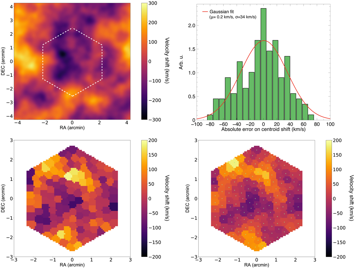
Example of simulated velocity fields. Top left: example of an emission-measure weighted projection of the simulated line-of-sight component of the turbulent velocity field. In this case k_inj = 1/150 kpc⁻¹ and k_dis = 1/20 kpc⁻¹. The shape and the extent of the X-IFU FoV is shown as a white dashed line. Top right: absolute error distribution between the recovered line-of-sight velocity in one of the simulations and the corresponding input emission-measure-weighted velocity. The statistical error follows a centred Gaussian distribution where the Gaussian best fit (in red) is found for μ_stat = 0.2 km s⁻¹ and σ_stat, C = 34 km s⁻¹. Bottom left: example of a synthetic X-IFU observation of bulk motion for k_inj = 1/200 kpc⁻¹ and k_dis = 1/10 kpc⁻¹ and (bottom right) corresponding emission-measure weighted input map (binned). The small green crosses indicate the centres of the Voronoï regions.