| Issue |
A&A
Volume 629, September 2019
|
|
|---|---|---|
| Article Number | A46 | |
| Number of page(s) | 8 | |
| Section | Cosmology (including clusters of galaxies) | |
| DOI | https://doi.org/10.1051/0004-6361/201935213 | |
| Published online | 03 September 2019 | |
Breaking cosmic degeneracies: Disentangling neutrinos and modified gravity with kinematic information
1
Oskar Klein Centre, Department of Physics, Stockholm University, 106 91 Stockholm, Sweden
e-mail: This email address is being protected from spambots. You need JavaScript enabled to view it.
2
Excellence Cluster Universe, Boltzmannstr. 2, 85748 Garching, Germany
3
Universitäts-Sternwarte, Fakultät für Physik, Ludwig-Maximilians Universität München, Scheinerstr. 1, 81679 München, Germany
4
Department of Physics, University of California, Santa Barbara, CA 93106, USA
5
Institute of Theoretical Astrophysics, University of Oslo, Postboks 1029, Blindern 0315, Oslo, Norway
6
Dipartimento di Fisica e Astronomia, Alma Mater Studiorum Università di Bologna, Via Gobetti 93/1, 40129 Bologna, Italy
7
Astrophysics and Space Science Observatory Bologna, Via Gobetti 93/2, 40129 Bologna, Italy
8
INFN – Sezione di Bologna, Viale Berti Pichat 6/2, 40127 Bologna, Italy
Received:
5
February
2019
Accepted:
13
May
2019
Abstract
Searches for modified gravity in the large-scale structure try to detect the enhanced amplitude of density fluctuations caused by the fifth force present in many of these theories. Neutrinos, on the other hand, suppress structure growth below their free-streaming length. Both effects take place on comparable scales, and uncertainty in the neutrino mass leads to a degeneracy with modified gravity parameters for probes that are measuring the amplitude of the matter power spectrum. We explore the possibility to break the degeneracy between modified gravity and neutrino effects in the growth of structures by considering kinematic information related to either the growth rate on large scales or the virial velocities inside of collapsed structures. In order to study the degeneracy up to fully non-linear scales, we employ a suite of N-body simulations including both f(R) modified gravity and massive neutrinos. Our results indicate that velocity information provides an excellent tool to distinguish massive neutrinos from modified gravity. Models with different values of neutrino masses and modified gravity parameters possessing a comparable matter power spectrum at a given time have different growth rates. This leaves imprints in the velocity divergence, which is therefore better suited than the amplitude of density fluctuations to tell the models apart. In such models with a power spectrum comparable to ΛCDM today, the growth rate is strictly enhanced. We also find the velocity dispersion of virialised clusters to be well suited to constrain deviations from general relativity without being affected by the uncertainty in the sum of neutrino masses.
Key words: large-scale structure of Universe / galaxies: kinematics and dynamics
Hubble fellow.
© ESO 2019
1. Introduction
Nearly two decades after the first measurements of the accelerated expansion of space (e.g. Riess et al. 1998; Perlmutter et al. 1999; Schmidt et al. 1998) the fact that about 70% of the energy content of the Universe is in a form with a negative equation of state of w ≈ −1 has been confirmed in numerous measurements (Bennett et al. 2013; Planck Collaboration XIII 2016). Nevertheless, the nature of this “dark energy” is as puzzling as it has been since its discovery. Tremendous efforts in modern cosmology go into determining the amount and possible time evolution of this unknown component. It is particularly problematic that few well-motivated frameworks for its physical nature exist apart from a cosmological constant. Many ideas (e.g. Dvali et al. 2000) have by now been ruled out or shown to be intrinsically unstable. While there are still theories around (and always will be, since the parameter space of many of these is very flexible), they contribute little to the understanding of underlying fundamental problems such as the absence of gravitational effects of vacuum energy.
It is also important to recall that gravity is the least well understood fundamental force, and a lot of implicit assumptions are being made when extrapolating our knowledge over several orders of magnitudes to vastly different conditions and scales. These two points are, in fact, the main motivations behind a class of modified gravity (MG) theories (Amendola & Tsujikawa 2010; Clifton et al. 2012). Since general relativity (GR) as a theory of gravity is unique under very general assumptions (Lovelock 1972), any modification introduces new physical degrees of freedom. These can lead to accelerated expansion, but also tend to enhance gravity on a perturbative level as so-called fifth forces. To pass observational bounds, any of these models have to involve a “screening mechanism” leading to negligible deviations in, for example the solar system where the predictions of GR have been confirmed to high precision (e.g. Bertotti et al. 2003; Will 2006).
In this work, we circumvent the discussion of what characterises a scientific theory (as opposed to, for instance, an effective theory), and instead treat the screened MG models considered as examples of a (much) larger group of models. These models all possess the common property that in addition to the Newtonian gravitational force FN, another fifth force component FFifth exists, which is suppressed by some screening mechanism in high-density (or high-curvature) environments. This choice is motivated by the fact that screening occurs in a range of scalar- and vector-field theories for various physical reasons, and is in fact essentially required by a large class of theories in order not to violate local gravity measurements. Examples of screening mechanisms which are implemented in those theories include
-
Chameleon (Khoury & Weltman 2004), in which the range of the fifth force is decreased in regions of high space-time curvature, thus, effectively hiding the additional force;
-
Symmetron (Hinterbichler & Khoury 2010; Hinterbichler et al. 2011), in which the coupling of the scalar field is density dependent;
-
Vainshtein screening (Vainshtein 1972), in which the screening effect is sourced by the second derivative of the field value; and
-
others such as screening through disformal coupling (Bekenstein 1993).
As already indicated above, a major problem in the search for a new theory of gravity is that ΛCDM so far only gets confirmed to higher and higher precision. While minor discrepancies between probes of the early and late Universe exist, especially in measurements of the Hubble parameter H0 (see e.g. Planck Collaboration VI 2018; Riess et al. 2019) and Ωm or σ8 (e.g. Hildebrandt et al. 2017; Abbott et al. 2018), no major tension between its predictions and the data has been found. Historically, however, we know that this does not mean that ΛCDM is correct but that either we have not yet found the right probe where tensions might arise, or we have to push the limits to higher precision. While the latter approach can well be fruitful, as shown by the high-precision measurements of for example the perihelion precession of Mercury (Le Verrier 1859) and is the preferred path taken by many next generation instruments such as Euclid (Refregier et al. 2010) and WFIRST1 (Spergel et al. 2015), we focus on the former path, and are thus interested in deviations on the ≳10% level.
Several observable signatures of screened MG models have been suggested in the literature such as deviations in the halo mass function (Schmidt 2010; Davis et al. 2012; Puchwein et al. 2013; Achitouv et al. 2016) or the structure of the cosmic web (Falck et al. 2014; Ho et al. 2018). However one concern raised by several authors (e.g. Motohashi et al. 2013; He 2013; Baldi et al. 2014) is that massive neutrinos and beyond-ΛCDM models might be degenerate.
In this work, we want to investigate how kinematic information can be used to break these degeneracies. This paper is structured as follows: in Sect. 2 we introduce the screened MG models studied and briefly review the effect of neutrinos on structure formation. We also describe our numerical simulations used to explore the joint effects numerically. In Sect. 3 we present our results, before we conclude in Sect. 4.
2. Method
This section briefly summarises the effects of MG and massive neutrinos on the evolution of the density field. We also present the simulation suite used to study the combined effects in the fully non-linear regime.
2.1. Review of modified gravity
To work within a well-defined framework, in this paper we focus on f(R) gravity. As a starting point we assume the generalised Einstein-Hilbert action2
 (1)
(1)
where we introduce a function f of the Ricci scalar R, the Lagrangian ℒm contains all other matter fields, and we recover standard GR if we choose the function to be a cosmological constant f = −2ΛGR. For this paper, we instead use the form established by Hu & Sawicki (2007)
 (2)
(2)
with a constant suggestively named Λ and an additional scale m2 that both have to be fixed later on. Assuming m2 ≪ R lets us expand the function
 (3)
(3)
with the background value of the Ricci scalar  today and we define the dimensionless parameter
  that expresses the deviation from GR. We return to the characteristic scale of fR0 later, but typically |fR0|≪1. The constant Λ = ΛGR is then fixed to the measured value of the cosmological constant by the requirement to reproduce the standard ΛCDM expansion history established by observations. However, we note that it no longer has the interpretation of a vacuum energy. The phenomenology of the theory in this limit is then set by fR0 alone. This particular choice of parameters also implies that the background evolution is indistinguishable from a ΛCDM universe, but the growth of perturbations differs.
To work out the perturbation equations, we vary the action with respect to the metric to arrive at the modified Einstein equations
 (4)
(4)
The new dynamical scalar degree of freedom fR ≡ df/dR is responsible for the modified dynamics of the theory. To obtain the equation of motion for this scalar field, we consider the trace of Eq. (4)
 (5)
(5)
where a is the scale factor of the metric; we assume the field to vary slowly (the quasi-static approximation) and consider small perturbations  ,
,  and
and  on a homogeneous background. To get a Poisson-like equation for the scalar metric perturbation 2ψ = δg00/g00 we take the time-time component of Eq. (4) to arrive at
 (6)
(6)
that now also depends on the scalar field. Solving the non-linear Eqs. (5) and (6) in their full generality requires N-body simulations, but it is interesting to consider two edge cases to get some insight into the phenomenology of the theory.
If the field is large, |fR0|≫|ψ|, we can expand
 (7)
(7)
and we can solve Eqs. (5) and (6) in Fourier space to get
 (8)
(8)
with the Compton wavelength of the scalar field μ−1 = (3dfR/dR)1/2. For k ≫ μ the second term vanishes and we obtain a Poisson equation with an additional factor 4/3. On the other hand, for k ≪ μ we recover standard gravity. The Compton wavelength μ−1 therefore sets the interaction range of an additional fifth force that enhances gravity by one-third.. This is the maximum possible force enhancement in f(R), irrespective of the choice of the function in Eq. (2).
For field values |fR0|≪|ψ|, the two terms on the right hand side of Eq. (5) approximately cancel, so we arrive at
 (9)
(9)
and we also recover the standard Poisson equation from Eq. (6). This is the Chameleon screening mechanism mentioned above to restore GR in regions of high curvature.
We can get an estimate of the scale where this screening transition occurs by solving Eq. (5) formally with the appropriate Green’s function
 (10)
(10)
 (11)
(11)
where we defined the effective mass term Meff acting as a source for the fluctuations in the scalar field δfR. This definition requires Meff(r) ≤ M(r), and both contributions are equal in the unscreened regime, where Eq. (9) implies Meff = M. In this case, δfR = 2/3ψN with the Newtonian potential of the overdensity, ψN = GM/r. Since we assumed small perturbations on the homogeneous background,  , we arrive at the screening condition
 (12)
(12)
In other words, only the mass distribution outside of the radius where the equality 2/3ψ(r) = |fR| holds contributes to the fifth force. We note that screening for real halos is considerably more complex, since non-sphericity and environmental effects are also important for the transition. Nevertheless, Eq. (12) gives a reasonable estimate for the onset of the transition between enhanced gravity and normal GR.
Since screening can function only for ψN ∼ fR, the condition implied by Eq. (12) sets the scale for the free parameter |fR0|. Typical values for the metric perturbation in cosmology range from ψN ∼ 10−5 to ψN ∼ 10−6, so |fR0| should be of the same order of magnitude to show any interesting phenomenology. For values of the scalar field |fR0|≫ψN, gravity is always enhanced so we can exclude this parameter space trivially, while in the opposite limit |fR0|≪ψ the theory is always screened and does not offer any predictions to distinguish it from GR on cosmological scales.
2.2. Neutrino effects on structure growth
Cosmology allows us to constrain the physics of neutrinos in unique ways. Assuming the standard thermal evolution and decoupling before e+/e− annihilation, their temperature is related to that of the cosmic microwave background (CMB) photons by
 (13)
(13)
which implies for neutrinos with mass eigenstates mν a total contribution to the energy budget of the Universe of (Mangano et al. 2005)
 (14)
(14)
where the sum runs over the three standard model neutrino states. Since the mass of neutrinos is constrained to be small, ∑mν ≲ 1 eV, they decouple as highly relativistic particles in the early Universe. The energy density of neutrinos therefore scales as an additional radiation component Ων ∝ a−4 early on, but during adiabatic cooling with the expansion of the Universe they become non-relativistic and the energy density behaves like ordinary matter Ων ∝ a−3 today. The small contribution from Eq. (14) to the overall energy budget also implies that their effect on the background expansion history is small.
Their weak interaction cross-section makes neutrinos a dark matter component. However, compared to the standard cold dark matter (CDM), they have considerable bulk velocities. This changes the growth of perturbations on scales smaller than the distance travelled by neutrinos up to today, the neutrino horizon, defined by
 (15)
(15)
with the average neutrino velocity cν, which is close to the speed of light early on. The neutrino horizon itself is numerically closely related to the more commonly used free-streaming wavenumber at the time of the non-relativistic transition, knr (Lesgourgues et al. 2013)
 (16)
(16)
where Ωm denotes the current matter density parameter. On scales exceeding the neutrino horizon, velocities can be neglected and the perturbations consequently evolve identically to those in the cold dark matter component. For smaller scales k ≫ knr within the neutrino horizon, however, free-streaming leads to slower growth of neutrino perturbations. Because of gravitational back-reaction on the other species, this causes a characteristic step-like suppression of the linear matter power spectrum approximately given by (Hu et al. 1998)
 (17)
(17)
To compare the density power spectrum between cosmologies with and without neutrinos, we assumed the same primordial perturbations and kept the total Ωm (including neutrinos) fixed, resulting in equal positions of the peak of the power spectrum and ensuring that the spectra are identical in the super-horizon limit. The cosmologies for our neutrino simulations described in Sect. 2.3 are chosen in the same way.
The interplay between neutrinos and f(R) gravity is interesting owing to a curious coincidence: the typical range of the fifth force given by the Compton wavelength μ−1 in Eq. (8) and the free-streaming scale of neutrinos in Eq. (16) are comparable for the relevant parameter space of neutrino masses and values of |fR0|, such that the known standard model neutrinos might counteract signatures of boosted growth caused by MG. This makes neutrinos important for constraints on f(R), and this paper searches for ways to disentangle both effects.
2.3. DUSTGRAIN-pathfinder simulations
Our analysis is based on a subset of the DUSTGRAIN-pathfinder simulations suite described in Giocoli et al. (2018). The main purpose of the DUSTGRAIN-pathfinder simulations is to explore the degeneracy between neutrino and MG effects by sampling the joint f(R)−∑mν parameter space with combined N-body simulations that simultaneously implement both effects in the evolution of cosmic structures. To this end, the MG-GADGET code – specifically developed by Puchwein et al. (2013) for f(R) gravity simulations – has been combined with the particle-based implementation of massive neutrinos described in Viel et al. (2010), allowing us to include a separate family of neutrino particles to the source term of the δfR field Eq. (5), which reads
 (18)
(18)
The DUSTGRAIN-pathfinder simulations follow the evolution of (2 × )7683 particles of dark matter (and massive neutrinos) in a periodic cosmological box of 750 h−1 Mpc per side from a starting redshift of zi = 99 to z = 0, for a variety of combinations of the parameters |fR0| in the range [10−6,10−4] and ∑mν in the range [0.0,0.3] eV, plus a reference ΛCDM simulation (i.e. GR with ∑mν = 0). The cosmological parameters assumed in the simulations are consistent with the Planck 2015 constraints (see Planck Collaboration XIII 2016) ΩM = ΩCDM + Ωb + Ων = 0.31345, ΩΛ = 0.68655, h = 0.6731, σ8(ΛCDM) = 0.842. The dark matter particle mass (for the massless neutrino cases) is MCDM = 8.1 × 10¹⁰ h−1 M⊙ and the gravitational softening is set to ϵg = 25 h−1 kpc, corresponding to (1/40) times the mean inter-particle separation.
We generated the initial conditions for the simulations by following the Zel’dovich approximation to generate a random realisation of the linear matter power spectrum obtained with the Boltzmann code CAMB3 (Lewis et al. 2000) for the cosmological parameters defined above and under the assumption of standard GR. For the simulations including massive neutrinos, besides updating the CAMB linear power spectrum used to generate the initial conditions accordingly, we also employed the approach described in Zennaro et al. (2017) and Villaescusa-Navarro et al. (2018). This amounts to generating two fully correlated random realisations of the linear matter power spectrum for standard cold dark matter particles and massive neutrinos based on their individual transfer functions. Neutrino thermal velocities are then randomly sampled from the corresponding Fermi distribution and added on top of gravitational velocities to the neutrino particles. We used the same random seeds to generate all initial conditions to suppress cosmic variance in the direct comparison between models. As the simulations start at zi = 99 when f(R) effects are expected to be negligible, no modifications are necessary to incorporate MG into the initial conditions and the standard GR particle distributions – with and without neutrinos – can be safely employed for both the GR and f(R) runs.
A summary of the main parameters of the simulations considered in this work is presented in Table 1. Giocoli et al. (2018) provide a more detailed description of the DUSTGRAIN-pathfinder simulations.
Summary of the main numerical and cosmological parameters characterising the subset of the DUSTGRAIN-pathfinder simulations considered in this work.
3. Cosmic degeneracies
The first N-body simulation to investigate the joint effects of neutrinos and MG was performed in Baldi et al. (2014) where the authors pointed out the degeneracy between the competing signals. This was confirmed by multiple recent papers based on simulations to study how neutrinos can mask f(R) imprints in the kinematic Sunyaev–Zeldovich effect of the large-scale structure (Roncarelli et al. 2017, 2018), weak lensing statistics (Giocoli et al. 2018; Peel et al. 2018), and the abundance of galaxy clusters (Hagstotz et al. 2019). A first attempt to exploit Machine Learning techniques to separate the two signals was put forward by Peel et al. (2019) and Merten et al. (2019).
All these studies confirm a degeneracy in observables that rely on structure growth, which makes the unknown neutrino masses an important nuisance parameter when constraining f(R) gravity, as pointed out in Hagstotz et al. (2019). These papers also show that especially the redshift evolution can be a potentially powerful tool in distinguishing these models since the time evolution of the modifications induced by f(R) and neutrinos differs in general. However, many large-scale structure data sets available today do not have sufficient redshift reach to set stringent constraints on deviations from GR while marginalising over neutrino mass.
We refer to the above cited papers for details how these degeneracies play out for various probes and how they can be broken with higher redshift data, but the main challenge is summarised in Fig. 1, where we show the relative change induced in the matter power spectrum (left) and the halo abundance (right). We note that even though the halo mass function is clearly derived from the matter power spectrum, the degeneracy in the cluster abundance demonstrated here is non-trivial since the threshold of collapse δc also changes in f(R) gravity (e.g. Schmidt et al. 2009; Kopp et al. 2013; Cataneo et al. 2016; von Braun-Bates et al. 2017). Within current observational accuracy, the effect of MG leading to additional structure growth and the suppression effect of neutrino free-streaming are thus difficult to distinguish. Therefore, extending the cosmological parameter space with free neutrino masses tends to weaken existing limits on |fR0|.
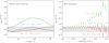 |
Fig. 1. Left: relative deviation induced by f(R) gravity and massive neutrinos in the matter power spectrum measured in a subset of our simulations at z = 0. The large deviation caused by the additional growth in |fR0| = 10−4 is almost completely counteracted by massive neutrinos with ∑mν = 0.3 eV. We find a similar case for |fR0| = 10−5 and ∑mν = 0.15 eV. Right: same degeneracy in the simulated abundance of halos at z = 0. We note that the degeneracy is non-trivial; the same P(k) can lead to different cluster abundances in f(R) since the collapse threshold is changed in MG. The uncertainty for the cluster abundance is calculated with Poisson error bars. Shaded grey bands indicate the 10% deviation region in both plots. |
Since the degeneracy is broken by the different redshift evolution of the density δ in f(R) and neutrino cosmologies, it is interesting to consider the growth rate of structures to tell them apart. In linear theory, the continuity equation
 (19)
(19)
relates the growth rate f+ = dlnD+/dlna directly to the velocity divergence
 (20)
(20)
with the Hubble rate  , and we use θ as a probe of the different growth histories in GR, MG, and neutrino cosmologies. We then investigate the degeneracy between the latter in two regimes: First we discuss the large-scale velocity divergence two-point function in Fourier space Pθθ as a proxy for the growth rate and present the detailed results in Sect. 3.1. Then we turn towards the velocity dispersion of non-linear collapsed structures in Sect. 3.2.
3.1. Velocity divergence two-point functions
We compute the velocity divergence θ = 1/H∇⋅v and interpolate it on a uniform, 5123-point grid, using the publicly available Delaunay Tessellation Field Interpolation (DTFE4) code (Cautun & van de Weygaert 2011). The DTFE code uses the Delaunay Density Estimator Method – a volume-weighted (as opposed to mass-weighted) interpolation technique which preserves sharp density contrasts (caused by e.g. filamentary structures) due to the tessellation. Another advantage of this interpolation technique is that it is automatically adaptive, that is, it samples higher density regions better than underdensities. For our usage this leads primarily to decreased computing time.
This interpolation allows us to compare the power spectrum Pθθ in the ΛCDM simulation with the f(R) and massive neutrino simulations in Fig. 2 where we plot (as in the left panel of Fig. 1 for the matter power spectrum) the relative deviation from the ΛCDM value. Clearly, all MG simulations show an increased velocity divergence – and therefore growth rate – on scales ≳0.1 Mpc h−1; the |fR0| = 10−4 simulation shows the strongest enhancement since the fifth force becomes active first. Very large scales k ≪ μ−1 exceeding the range of the force given by the Compton wavelength of the scalar field are not affected. These results confirm previous findings (see e.g. Jennings et al. 2012) that the velocity power spectrum provides a much stronger signature of MG compared to the density power spectrum, thereby representing a more powerful tool to test gravity on cosmological scales. In principle the velocity power spectrum can be probed by redshift space distortion measurements sensitive to f+σ8/b, assuming knowledge of the tracer bias b (Peacock et al. 2001; Alam et al. 2017). However, the scale dependence of f+ in MG, changes in galaxy formation, and subsequently the tracer bias, and difficult modelling of the non-linear effects in MG make this analysis challenging (see the discussion in Jennings et al. 2012; Hernández-Aguayo et al. 2019).
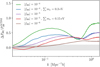 |
Fig. 2. Relative change in the velocity divergence power spectrum Pθθ compared to ΛCDM for various models with MG, massive neutrinos, or both. The deviation from ΛCDM is more pronounced compared to the approximately degenerate density power spectra for combinations of |fR0| and ∑mν shown in Fig. 1. The dip in the spectra marks the onset of collapsed structures. The shaded band indicates a 10% deviation range. |
The addition of neutrinos (cf. the two |fR0| = 10−5 runs in Fig. 1) dampens the velocity divergence field slightly overall, but unlike for the density power spectrum this effect is not sufficient to counteract the enhanced growth rate in f(R). This confirms the redshift evolution of the degeneracy in the density field: at early times z ≳ 0.5, f(R) effects are small, and neutrino suppression of the matter fluctuations dominates. As soon as the additional force enhancement becomes active, it tends to win out and we arrive at the approximate degeneracy currently observed as shown in Fig. 1. In the future evolution, f(R) effects will dominate over the neutrino damping for the cases shown here.
The plot also demonstrates that hierarchical formation of collapsed objects in f(R) proceeds faster than in a ΛCDM universe. Small structures form first and this process proceeds to larger scales with time. Since the fifth force accelerates the collapse, cosmologies with higher values of |fR0| contain larger non-linear structures at a given redshift z. The transition to these collapsed structures appears as a characteristic dip in the velocity divergence power spectrum (see also the detailed explanation in Li et al. 2013).
3.2. Cluster velocity dispersion
We now turn to the kinematics inside of non-linear structures. The velocity dispersion of galaxy cluster members is a long-established measure of the total gravitational potential via the virial theorem, and therefore this measure can serve as a mass proxy of the system (Biviano et al. 2006). The first studies of f(R) effects on virialised systems were presented by Lombriser et al. (2012), and recently efforts have been made to use the phase-space dynamics of single massive clusters to constrain MG (e.g. Pizzuti et al. 2017).
We focus on the change in the mean observable velocity dispersion instead of detailed studies of single objects. The starting point is the virial theorem, which itself is a consequence of phase-space conservation expressed by the Liouville equation and holds for any system obeying Hamiltonian dynamics. It is therefore unchanged by f(R) gravity, and states in its scalar form
 (21)
(21)
with kinetic and potential energy of the system, respectively. From there, we can get a rough estimate for the velocity dispersion
 (22)
(22)
for a virialised system of size r. This makes the velocity dispersion a direct measurement of the gravitational potential of a bound system. For an unscreened cluster in f(R), Eq. (8) leads to an enhancement of the gravitational force and potential by a factor 4/3; we therefore expect the velocity dispersion to be boosted by (4/3)1/2 compared to the standard prediction.
However, the screening mechanism of f(R) gravity outlined in Sect. 2.1 is crucial to understand the full phenomenology of the theory. We can estimate the mass scale of objects with potential wells deep enough to activate the screening mechanism with the condition set by Eq. (12). In order to do that, we consider the force enhancement caused by f(R)
 (23)
(23)
relative to the Newtonian potential ψN. We can from there calculate the average additional potential energy of the system
 (24)
(24)
which varies between 1 (for the screened case) and 4/3 (for the unscreened case), where the weighting function
 (25)
(25)
Following Schmidt (2010), we assume that the additional force is only sourced by the mass distribution beyond the screening radius rscreen, which is defined by the equality in condition Eq. (12), i.e.
 (26)
(26)
This implies for the force enhancement
 (27)
(27)
and since we are considering the average behaviour of halos, we can solve the equations above by assuming Navarro–Frenk–White (Navarro et al. 1996) density profiles to determine  . We use the concentration-mass relation by Bullock et al. (2001) to fix the density profiles, but the overall results for
  are rather insensitive to the specific choice of c(M, z). From the modified potential energy, the virial theorem then suggests the scaling of the velocity dispersion σ in f(R) as
 (28)
(28)
The screening radius rscreen itself depends on time via the evolution of the density profile c(M, z) and the background evolution of the scalar field
 (29)
(29)
The velocity dispersion measured in our simulations at z = 0 is plotted in Fig. 3, where the width of the contours represents the standard deviation found among the objects. Most of the clusters virialise either to the ΛCDM equilibrium or the boosted f(R) value, and since the maximum force enhancement is identical for all models, |fR0| merely determines at which mass scale the transition between the two cases occurs. We also show results for the simulation with |fR0| = 10−5 and ∑mν = 0.15 eV as an example of a cosmology with both MG and massive neutrinos, but we note that neutrinos have no detectable effect on the cluster velocity dispersion. Therefore the dynamics of galaxies within clusters are an excellent way to break the degeneracy found in measurements relying on the amplitude of the matter fluctuations.
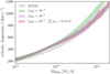 |
Fig. 3. Velocity dispersion σ within clusters of a given mass M200m for a subset of the studied cosmologies at z = 0. The shaded region shows the standard deviation found in our simulations. We note that most systems are virialised, either to the ΛCDM value or the boosted unscreened f(R) equilibrium. Neutrinos do not have any detectable effect on the velocity dispersion inside of clusters, and we just show the case with |fR0| = 10−5 and ∑mν = 0.15 eV for clarity. The relative deviations are shown separately in Fig. 4. |
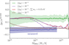 |
Fig. 4. Relative velocity dispersion within clusters of a given mass in the extended cosmologies, normalised to the mean value of the ΛCDM simulation. The (propagated) error bar of the ratio Δσ/σ is showcased for the |fR0| = 10−4 model as the shaded region, and has a similar magnitude for all curves. The other error bars are suppressed for clarity. Also shown is the empirical relation (blue) with propagated error bars as described in the text. Dashed lines show the expectation |


We focus on the relative deviations from ΛCDM in Fig. 4, where we normalise the curves to the values measured in our fiducial simulation. Dashed lines show the prediction  from Eq. (24).
Clusters for |fR0| = 10−4 are all unscreened and virialise to the f(R) equilibrium value boosted by a factor (4/3)1/2 ≈ 1.15. On the other hand |fR0| = 10−6 is almost completely screened, and just shows slight deviations for low mass systems with M200m ∼ 1013 M⊙ h−1. The intermediate case |fR0| = 10−5 demonstrates how the screening mechanism becomes active for clusters with M200m ∼ 2 × 10¹⁴ M⊙ h−1 with a long transition tail towards the fully screened regime. This also implies that single very massive clusters are not well suited to constrain f(R) models (see e.g. Pizzuti et al. 2017, for a case study).
The simple model from Eq. (24) somewhat overestimates the efficiency of the screening mechanism, in agreement with findings by Schmidt (2010). It therefore only serves as a conservative estimate for the transition region. In addition, even clusters that are screened today can still carry the imprint of the fifth force if parts of the progenitor structures were unscreened in their past. The relaxation time of a galaxy cluster of richness N is approximately given by (Binney & Tremaine 2008)
 (30)
(30)
where typical crossing times tcross ≈ 1 Gyr; this leads to relaxation timescales of order tr ≈ 2 Gyr for a richness N ∼ 100 and can range up to the Hubble time tr ≈ 14.5 Gyr for very massive clusters with N ∼ 1000 member galaxies.
We also compare the results found in the simulations to an empirical σ(M) relation, which we obtained by combining the mass-richness relation of Johnston et al. (2007) and the σ-richness relation of Becker et al. (2007). Both studies used the catalogue of the Sloan Digital Sky Survey (SDSS; Sheldon et al. 2009), which allowed us to combine the two empirical relations. Specifically, we used their fit to the data relating the cluster richness N (i.e. the number of detected galaxies per cluster) and the mass. Becker et al. (2007) and Johnston et al. (2007) estimated kinematic and lensing mass measurements, respectively. The uncertainty shown in Fig. 4 is the (propagated) uncertainty quoted in these studies.
Even without giving a quantitative upper limit on fR0 here, we note that the |fR0| = 10−5 results seem to be incompatible with the observed cluster velocity dispersion irrespective of neutrino effects. This is comparable to current upper limits obtained from large-scale structure data (e.g. Cataneo et al. 2015).
4. Conclusions
Neutrinos are of great interest for MG searches in the large-scale structure since they suppress the growth of structures on scales comparable to the range of the fifth force expected in deviations from GR. The uncertainty in the neutrino mass scale leads to an uncertainty in the size of this suppression, which can mask the characteristic additional growth of structures in f(R) gravity. This degeneracy was studied before in the context of the amplitude of matter fluctuations and found to be time dependent, since the modifications in the growth of structures induced by neutrinos and the fifth force have different redshift dependencies.
Therefore, in this paper we studied the velocity divergence power spectrum Pθθ in Sect. 3.1 as a proxy for the linear growth rate. Compared to ΛCDM it is strictly enhanced in our simulations at z = 0, as well as in cosmologies including both MG and massive neutrinos that show a comparable amplitude of matter fluctuations at that time. We conclude that for combinations of parameters that show approximate degeneracy in the current matter power spectrum, neutrino suppression dominates in the past, while in the future evolution the additional growth induced by the fifth force will win out. This effect can be probed by redshift-space distortion measurements, but an analysis accounting for the scale dependent growth in f(R) remains challenging (Jennings et al. 2012; Hernández-Aguayo et al. 2019).
As a second step, we studied the kinematics inside of clusters in Sect. 3.2. The velocity dispersion found in our simulations agrees well with the expectations from the virial theorem, and it is enhanced in the unscreened f(R) regime by a factor (4/3)1/2 proportional to the maximum force enhancement. Neutrinos on the other hand do not have any detectable effect on the velocity dispersion. Since the free-streaming length is larger than the typical cluster size, neutrinos behave as a smooth background component. So while they suppress the overall cluster abundance, the kinematics inside of halos are completely unaffected. We also compare the simulated dynamics to the empirical σ − M relation found by combining the results from Johnston et al. (2007) and Becker et al. (2007) and find good agreement with the ΛCDM simulation. While we do not find a stringent upper limit on the modified gravitiy parameter |fR0|, we point out that the observed relation is in strong tension with expectations from an |fR0| = 10−5 model for clusters of mass M200m ≈ 10−14 M⊙ h−1, i.e., independent of the neutrino mass.
Overall, kinematic information is an excellent observable to detect fifth force effects irrespective of the unknown neutrino mass. Using kinematic information could also be potentially useful to break other degeneracies with (screened) MG theories such as baryonic feedback processes stemming, for example from active galactic nucleis, which also reduce clustering (Arnold et al. 2014; Ellewsen et al. 2018).
Wide Field Infrared Survey Telescope.
We adopt natural units c = ℏ = 1.
Acknowledgments
Many cosmological quantities in this paper were calculated using the Einstein-Boltzmann code CLASS (Blas et al. 2011). We appreciate the help of Ben Moster with cross-checks for our simulation suite and helpful discussions with Raffaella Capasso on cluster dynamics. SH acknowledges the support of the DFG Cluster of Excellence “Origin and Structure of the Universe” and the Transregio programme TR33 “The Dark Universe”. MG was supported by by NASA through the NASA Hubble Fellowship grant #HST-HF2-51409 awarded by the Space Telescope Science Institute, which is operated by the Association of Universities for Research in Astronomy, Inc., for NASA, under contract NAS5-26555. MB acknowledges support from the Italian Ministry for Education, University and Research (MIUR) through the SIR individual grant SIMCODE (project number RBSI14P4IH), from the grant MIUR PRIN 2015 “Cosmology and Fundamental Physics: illuminating the Dark Universe with Euclid”, and from the agreement ASI n.I/023/12/0 “Attivita” relative alla fase B2/C per la missione Euclid. The DUSTGRAIN-pathfinder simulations discussed in this work have been performed and analysed on the Marconi supercomputing machine at Cineca thanks to the PRACE project SIMCODE1 (grant nr. 2016153604, P.I. M. Baldi) and on the computing facilities of the Computational Centre for Particle and Astrophysics (C2PAP) and the Leibniz Supercomputing Centre (LRZ) under the project ID pr94ji. We thank the Research Council of Norway for their support. Some computations were performed on resources provided by UNINETT Sigma2 – the National Infrastructure for High Performance Computing and Data Storage in Norway. This paper is partly based upon work from the COST action CA15117 (CANTATA), supported by COST (European Cooperation in Science and Technology).
References
- Abbott, T. M. C., Abdalla, F. B., Alarcon, A., et al. 2018, Phys. Rev. D, 98, 043526 [Google Scholar]
- Achitouv, I., Baldi, M., Puchwein, E., & Weller, J. 2016, Phys. Rev. D, 93, 103522 [CrossRef] [Google Scholar]
- Alam, S., Ata, M., Bailey, S., et al. 2017, MNRAS, 470, 2617 [NASA ADS] [CrossRef] [Google Scholar]
- Amendola, L., & Tsujikawa, S. 2010, Dark Energy: Theory and Observations (Cambridge: Cambridge University Press) [Google Scholar]
- Arnold, C., Puchwein, E., & Springel, V. 2014, MNRAS, 440, 833 [NASA ADS] [CrossRef] [Google Scholar]
- Baldi, M., Villaescusa-Navarro, F., Viel, M., et al. 2014, MNRAS, 440, 75 [NASA ADS] [CrossRef] [Google Scholar]
- Becker, M. R., McKay, T. A., Koester, B., et al. 2007, ApJ, 669, 905 [NASA ADS] [CrossRef] [Google Scholar]
- Bekenstein, J. D. 1993, Phys. Rev. D, 48, 3641 [NASA ADS] [CrossRef] [MathSciNet] [Google Scholar]
- Bennett, C., Hill, R. S., Hinshaw, G., et al. 2013, ApJS, 208, 20 [Google Scholar]
- Bertotti, B., Iess, L., & Tortora, P. 2003, Nature, 425, 374 [NASA ADS] [CrossRef] [PubMed] [Google Scholar]
- Binney, J., & Tremaine, S. 2008, Galactic Dynamics, 2nd edn. (Princeton: Princeton University Press) [Google Scholar]
- Biviano, A., Murante, G., Borgani, S., et al. 2006, A&A, 456, 23 [NASA ADS] [CrossRef] [EDP Sciences] [Google Scholar]
- Blas, D., Lesgourgues, J., & Tram, T. 2011, JCAP, 7, 034 [NASA ADS] [CrossRef] [Google Scholar]
- Bullock, J. S., Kolatt, T. S., Sigad, Y., et al. 2001, MNRAS, 321, 559 [Google Scholar]
- Cataneo, M., Rapetti, D., Schmidt, F., et al. 2015, Phys. Rev. D, 92, 044009 [NASA ADS] [CrossRef] [Google Scholar]
- Cataneo, M., Rapetti, D., Lombriser, L., & Li, B. 2016, JCAP, 12, 024 [CrossRef] [Google Scholar]
- Cautun, M. C., & van de Weygaert, R. 2011, The DTFE Public Software: The Delaunay Tessellation Field Estimator Code [Google Scholar]
- Clifton, T., Ferreira, P. G., Padilla, A., & Skordis, C. 2012, Phys. Rep., 513, 1 [NASA ADS] [CrossRef] [MathSciNet] [Google Scholar]
- Davis, A.-C., Li, B., Mota, D. F., & Winther, H. A. 2012, ApJ, 748, 61 [NASA ADS] [CrossRef] [Google Scholar]
- Dvali, G., Gabadadze, G., & Porrati, M. 2000, Phys. Lett. B, 485, 208 [NASA ADS] [CrossRef] [MathSciNet] [Google Scholar]
- Ellewsen, T. A. S., Falck, B., & Mota, D. F. 2018, A&A, 615, A134 [CrossRef] [EDP Sciences] [Google Scholar]
- Falck, B., Koyama, K., Zhao, G.-B., & Li, B. 2014, JCAP, 7, 058 [NASA ADS] [CrossRef] [Google Scholar]
- Giocoli, C., Baldi, M., & Moscardini, L. 2018, MNRAS, 481, 2813 [NASA ADS] [CrossRef] [Google Scholar]
- Hagstotz, S., Costanzi, M., Baldi, M., & Weller, J. 2019, MNRAS, 486, 3927 [CrossRef] [Google Scholar]
- He, J.-H. 2013, Phys. Rev. D, 88, 103523 [NASA ADS] [CrossRef] [Google Scholar]
- Hernández-Aguayo, C., Hou, J., Li, B., Baugh, C. M., & Sánchez, A. G. 2019, MNRAS, 485, 2194 [CrossRef] [Google Scholar]
- Hildebrandt, H., Viola, M., Heymans, C., et al. 2017, MNRAS, 465, 1454 [Google Scholar]
- Hinterbichler, K., & Khoury, J. 2010, Phys. Rev. Lett., 104, 231301 [NASA ADS] [CrossRef] [Google Scholar]
- Hinterbichler, K., Khoury, J., Levy, A., & Matas, A. 2011, Phys. Rev. D, 84, 103521 [NASA ADS] [CrossRef] [Google Scholar]
- Ho, A., Gronke, M., Falck, B., & Mota, D. F. 2018, A&A, 619, A122 [CrossRef] [EDP Sciences] [Google Scholar]
- Hu, W., & Sawicki, I. 2007, Phys. Rev. D, 76, 064004 [CrossRef] [Google Scholar]
- Hu, W., Eisenstein, D. J., & Tegmark, M. 1998, Phys. Rev. Lett., 80, 5255 [NASA ADS] [CrossRef] [Google Scholar]
- Jennings, E., Baugh, C. M., Li, B., Zhao, G.-B., & Koyama, K. 2012, MNRAS, 425, 2128 [NASA ADS] [CrossRef] [Google Scholar]
- Johnston, D. E., Sheldon, E. S., Wechsler, R. H., et al. 2007, ArXiv e-prints [arXiv:0709.1159] [Google Scholar]
- Khoury, J., & Weltman, A. 2004, Phys. Rev. D, 69, 044026 [CrossRef] [Google Scholar]
- Kopp, M., Appleby, S. A., Achitouv, I., & Weller, J. 2013, Phys. Rev. D, 88, 084015 [CrossRef] [Google Scholar]
- Lesgourgues, J., Mangano, G., Miele, G., & Pastor, S. 2013, Neutrino Cosmology (Cambridge: Cambridge University Press) [CrossRef] [Google Scholar]
- Le Verrier, U. 1859, Comptes rendus hebdomadaires des séances de l’Académie des sciences, 49, 379 [Google Scholar]
- Lewis, A., Challinor, A., & Lasenby, A. 2000, ApJ, 538, 473 [NASA ADS] [CrossRef] [Google Scholar]
- Li, B., Hellwing, W. A., Koyama, K., et al. 2013, MNRAS, 428, 743 [NASA ADS] [CrossRef] [Google Scholar]
- Lombriser, L., Koyama, K., Zhao, G.-B., & Li, B. 2012, Phys. Rev. D, 85, 124054 [NASA ADS] [CrossRef] [Google Scholar]
- Lovelock, D. 1972, J. Math. Phys., 13, 874 [NASA ADS] [CrossRef] [MathSciNet] [Google Scholar]
- Mangano, G., Miele, G., Pastor, S., et al. 2005, Nucl. Physics B, 729, 221 [Google Scholar]
- Merten, J., Giocoli, C., Baldi, M., et al. 2019, MNRAS, 487, 104 [CrossRef] [Google Scholar]
- Motohashi, H., Starobinsky, A. A., & Yokoyama, J. 2013, Phys. Rev. Lett., 110, 121302 [NASA ADS] [CrossRef] [Google Scholar]
- Navarro, J. F., Frenk, C. S., & White, S. D. M. 1996, ApJ, 462, 563 [NASA ADS] [CrossRef] [Google Scholar]
- Peacock, J. A., Cole, S., Norberg, P., et al. 2001, Nature, 410, 169 [NASA ADS] [CrossRef] [PubMed] [Google Scholar]
- Peel, A., Pettorino, V., Giocoli, C., Starck, J.-L., & Baldi, M. 2018, A&A, 619, A38 [NASA ADS] [CrossRef] [EDP Sciences] [Google Scholar]
- Peel, A., Lalande, F., Starck, J.-L., et al. 2019, Phys. Rev. D, 100, 023508 [CrossRef] [Google Scholar]
- Perlmutter, S., Aldering, G., Goldhaber, G., et al. 1999, ApJ, 517, 565 [NASA ADS] [CrossRef] [Google Scholar]
- Pizzuti, L., Sartoris, B., Amendola, L., et al. 2017, JCAP, 7, 023 [CrossRef] [Google Scholar]
- Planck Collaboration XIII. 2016, A&A, 594, A13 [NASA ADS] [CrossRef] [EDP Sciences] [Google Scholar]
- Planck Collaboration VI. 2018, A&A, submitted [arXiv:1807.06209] [Google Scholar]
- Puchwein, E., Baldi, M., & Springel, V. 2013, MNRAS, 436, 348 [NASA ADS] [CrossRef] [Google Scholar]
- Refregier, A., Amara, A., Kitching, T. D., et al. 2010, ArXiv e-prints [arXiv:1001.0061] [Google Scholar]
- Riess, A. G., Filippenko, A. V., Challis, P., et al. 1998, AJ, 116, 1009 [NASA ADS] [CrossRef] [Google Scholar]
- Riess, A. G., Casertano, S., Yuan, W., Macri, L. M., & Scolnic, D. 2019, ApJ, 876, 85 [NASA ADS] [CrossRef] [Google Scholar]
- Roncarelli, M., Villaescusa-Navarro, F., & Baldi, M. 2017, MNRAS, 467, 985 [Google Scholar]
- Roncarelli, M., Baldi, M., & Villaescusa-Navarro, F. 2018, MNRAS, 481, 2497 [CrossRef] [Google Scholar]
- Schmidt, B. P., Suntzeff, N. B., Phillips, M. M., et al. 1998, ApJ, 507, 46 [NASA ADS] [CrossRef] [Google Scholar]
- Schmidt, F. 2010, Phys. Rev. D, 81, 103002 [NASA ADS] [CrossRef] [Google Scholar]
- Schmidt, F., Vikhlinin, A., & Hu, W. 2009, Phys. Rev. D, 80, 083505 [NASA ADS] [CrossRef] [Google Scholar]
- Sheldon, E. S., Johnston, D. E., Scranton, R., et al. 2009, ApJ, 703, 2217 [NASA ADS] [CrossRef] [Google Scholar]
- Spergel, D., Gehrels, N., Baltay, C., et al. 2015, ArXiv e-prints [arXiv:1503.03757] [Google Scholar]
- Vainshtein, A. I. 1972, Phys. Lett. B, 39, 393 [Google Scholar]
- Viel, M., Haehnelt, M. G., & Springel, V. 2010, JCAP, 1006, 015 [CrossRef] [Google Scholar]
- Villaescusa-Navarro, F., Banerjee, A., Dalal, N., et al. 2018, ApJ, 61, 53 [NASA ADS] [CrossRef] [Google Scholar]
- von Braun-Bates, F., Winther, H. A., Alonso, D., & Devriendt, J. 2017, JCAP, 3, 012 [CrossRef] [Google Scholar]
- Will, C. M. 2006, Liv. Rev. Relativ., 9, 3 [NASA ADS] [CrossRef] [Google Scholar]
- Zennaro, M., Bel, J., Villaescusa-Navarro, F., et al. 2017, MNRAS, 466, 3244 [NASA ADS] [CrossRef] [Google Scholar]
All Tables
Summary of the main numerical and cosmological parameters characterising the subset of the DUSTGRAIN-pathfinder simulations considered in this work.
All Figures
|
Fig. 1. Left: relative deviation induced by f(R) gravity and massive neutrinos in the matter power spectrum measured in a subset of our simulations at z = 0. The large deviation caused by the additional growth in |fR0| = 10−4 is almost completely counteracted by massive neutrinos with ∑mν = 0.3 eV. We find a similar case for |fR0| = 10−5 and ∑mν = 0.15 eV. Right: same degeneracy in the simulated abundance of halos at z = 0. We note that the degeneracy is non-trivial; the same P(k) can lead to different cluster abundances in f(R) since the collapse threshold is changed in MG. The uncertainty for the cluster abundance is calculated with Poisson error bars. Shaded grey bands indicate the 10% deviation region in both plots. |
| In the text | |
|
Fig. 2. Relative change in the velocity divergence power spectrum Pθθ compared to ΛCDM for various models with MG, massive neutrinos, or both. The deviation from ΛCDM is more pronounced compared to the approximately degenerate density power spectra for combinations of |fR0| and ∑mν shown in Fig. 1. The dip in the spectra marks the onset of collapsed structures. The shaded band indicates a 10% deviation range. |
| In the text | |
|
Fig. 3. Velocity dispersion σ within clusters of a given mass M200m for a subset of the studied cosmologies at z = 0. The shaded region shows the standard deviation found in our simulations. We note that most systems are virialised, either to the ΛCDM value or the boosted unscreened f(R) equilibrium. Neutrinos do not have any detectable effect on the velocity dispersion inside of clusters, and we just show the case with |fR0| = 10−5 and ∑mν = 0.15 eV for clarity. The relative deviations are shown separately in Fig. 4. |
| In the text | |
|
Fig. 4. Relative velocity dispersion within clusters of a given mass in the extended cosmologies, normalised to the mean value of the ΛCDM simulation. The (propagated) error bar of the ratio Δσ/σ is showcased for the |fR0| = 10−4 model as the shaded region, and has a similar magnitude for all curves. The other error bars are suppressed for clarity. Also shown is the empirical relation (blue) with propagated error bars as described in the text. Dashed lines show the expectation |
| In the text | |
Current usage metrics show cumulative count of Article Views (full-text article views including HTML views, PDF and ePub downloads, according to the available data) and Abstracts Views on Vision4Press platform.
Data correspond to usage on the plateform after 2015. The current usage metrics is available 48-96 hours after online publication and is updated daily on week days.
Initial download of the metrics may take a while.