| Issue |
A&A
Volume 629, September 2019
|
|
|---|---|---|
| Article Number | A140 | |
| Number of page(s) | 8 | |
| Section | Stellar structure and evolution | |
| DOI | https://doi.org/10.1051/0004-6361/201935086 | |
| Published online | 17 September 2019 | |
The optical and NIR spectrum of the Crab pulsar with X-shooter
1
Department of Astronomy, The Oskar Klein Centre, Stockholm University, AlbaNova, 10691 Stockholm, Sweden
e-mail: This email address is being protected from spambots. You need JavaScript enabled to view it.
2
The Cosmic Dawn Center, Niels Bohr Institute, Copenhagen University, Vibenshuset, Lyngbyvej 2, 2100 Copenhagen, Denmark
3
Department of Astrophysics/IMAPP, Radboud University, PO Box 9010 6500 GL Nijmegen, The Netherlands
4
Department of Particle Physics and Astrophysics, Weizmann Institute of Science, Rehovot 7610001, Israel
Received:
16
January
2019
Accepted:
1
July
2019
Abstract
Context. Pulsars are well studied all over the electromagnetic spectrum, and the Crab pulsar may be the most studied object in the sky. Nevertheless, a high-quality optical to near-infrared (NIR) spectrum of the Crab or any other pulsar has not been published to date.
Aims. Obtaining a properly flux-calibrated spectrum enables us to measure the spectral index of the pulsar emission, without many of the caveats from previous studies. This was the main aim of this project, but in addition we could also detect absorption and emission features from the pulsar and nebula over an unprecedentedly wide wavelength range.
Methods. A spectrum was obtained with the X-shooter spectrograph on the Very Large Telescope. Special care was given to the flux-calibration of these data.
Results. A high signal-to-noise spectrum of the Crab pulsar was obtained from 300 nm to 2400 nm. The spectral index fit to this spectrum is flat with αν = 0.16 ± 0.07. For the emission lines we measured a maximum velocity of ∼1600 km s−1, whereas the absorption lines from the material between us and the pulsar is unresolved at the ∼50 km s−1 resolution. A number of diffuse interstellar bands and a few NIR emission lines that have previously not been reported from the Crab are highlighted.
Key words: pulsars: general / stars: neutron / ISM: lines and bands / pulsars: individual: Crab pulsar / ISM: supernova remnants
© ESO 2019
1. Introduction
The Crab pulsar is located in the middle of the Crab nebula (M1), the remnant of the supernova that occurred in the year 1054. This system is among the most- and best- studied astronomical objects in the sky, and the Crab pulsar itself often serves as the object against which other astronomical objects as well as instruments are gauged.
In the optical regime, only a dozen neutron stars have been detected, and optical pulsations are seen only for six of the several thousands known pulsars (Shearer & Golden 2002). When it comes to spectroscopic observations of pulsars in the optical regime, most optical pulsars are simply too faint, making such observations only marginally possible (for example, Vela pulsar, Mignani et al. 2007; PSR B0540−69, Serafimovich et al. 2004; Geminga, Martin et al. 1998 and PSR B0656+14, Zharikov et al. 2007).
On the other hand, the Crab pulsar is bright at V = 16.5 and is easily accessible with optical telescopes. It is thus the only pulsar for which a decent signal-to-noise spectrum can be obtained at optical wavelengths. Nevertheless, a complete optical to near-infrared (NIR) spectrum of this canonical object has been lacking.
Following the first optical spectrum of the Crab pulsar by Oke (1969) it took almost 30 years before a modern CCD spectrum was published Nasuti et al. (1996). This was followed by several investigations that provided data with medium-sized (2 − 4 m) telescopes more than 15 years ago (e.g., Sollerman et al. 2000; Carramiñana et al. 2000; Beskin & Neustroev 2001; Romani et al. 2001; Fordham et al. 2002). These observations were also followed by a series of theoretical papers aiming to interpret the optical emission (e.g., Björnsson et al. 2010; Massaro et al. 2006; O’Connor et al. 2005; Crusius-Wätzel 2001). Yet, while this is important from a theoretical perspective, the exact shape of the non-thermal optical-NIR spectral-energy-distribution (SED) of this isolated neutron star has remained elusive.
While we have previously studied the Crab pulsar SED from the ultraviolet regime with the Hubble Space Telescope (HST; Sollerman et al. 2000) to the NIR with the Very Large Telescope (VLT) and the Infrared Spectrometer And Array Camera (ISAAC; Sollerman 2003) as well as with the Nasmyth Adaptive Optics System Coude Near Infrared Camera (NACO; Sandberg & Sollerman 2009), few new attempts have been made to improve the observational quality of the Crab pulsar’s optical-NIR spectrum. The lack of a NIR spectrum for this canonical pulsar was surprising already 15 years ago (O’Connor et al. 2005), and the NIR SED has instead been patched together using photometric data (see Sollerman 2003; Sandberg & Sollerman 2009) from different instruments and occasions. Despite decades of observational and theoretical work, the Crab nebula and its pulsar still holds secrets and surprises, as reviewed by Hester (2008) and by Bühler & Blandford (2014).
In this paper, we present an X-shooter spectrum of the Crab pulsar. The main purpose with the X-shooter approach is to remedy the above-mentioned situation by obtaining the entire optical-NIR SED with a single instrument. The very wide wavelength coverage of the X-shooter spectrograph provides the complete U–K spectral energy distribution of the Crab pulsar at the same time. A coherent study of the non-thermal emission of an isolated neutron star could test the reality of the NIR self-absorption roll-over. Synchrotron self-absorption in the NIR regime has been suggested and invoked in pulsar models since the early 1970s, but the evidence for this in the Crab pulsar was questioned by Sandberg & Sollerman (2009). The actual value of the spectral index αν (we define the spectral index to be given as the power-law Fν ∝ ν+αν) of the pulsar in this region is also of importance for understanding the emission mechanism of pulsars. Björnsson et al. (2010) showed for example how the value of the spectral index in the optical-NIR regime translates to limits on the location of the emission zone within the pulsar magnetosphere.
This paper is organized as follows: observations and data reductions are presented in Sect. 2; spectroscopic analysis is provided in Sect. 3. Many of the caveats of pulsar optical spectroscopy are further discussed in Sect. 4; whereas a discussion of our results are given in Sect. 5. In Sect. 6 we present some additional science that can be done with these data, using absorption lines from the interstellar medium (ISM), diffuse interstellar bands (DIBs) and emission lines from the ejecta filaments. We summarize in Sect. 7. All X-shooter data presented in this paper are publicly available in the ESO archive and the fully reduced flux-calibrated spectrum is uploaded to WISeREP (Yaron & Gal-Yam 2012).
2. Observations and data reduction
The observations were obtained using the X-shooter echelle spectrograph (Vernet et al. 2011) mounted on the European Southern Observatory (ESO) 8.2m VLT, on Cerro Paranal in Chile. This is a multi-wavelength medium-resolution spectrograph that simultaneously obtains spectra with three different arms from the ultraviolet to the NIR. Each arm is an independent cross dispersed echelle with optics and detectors optimized for the aimed wavelength regimes. The total nominal wavelength coverage of the combined (3 arms) spectrum is 3000 − 24 000 Å. A log of the spectroscopic observations is given in Table 1, and the field observed in shown in Fig. 1.
Log of spectroscopic observations.
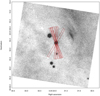 |
Fig. 1. An acquisition image of Crab pulsar and neighborhood from our X-shooter observations. The position angles provided in Table 1 are overlaid to show where the observations were obtained. The widths of the slits shown are 0 |

The strategy for these service mode observations were decided by the aim to obtain the best possible flux-calibrated data to work with. This was the main purpose and challenge in this study.
In our first observing run in 20141 we requested the observations to be obtained in dark or gray time under seeing conditions better than  and at maximum airmass of 1.7. Given the northern position of the Crab pulsar at declination +22°, the object actually does not rise higher than 43° above the Paranal horizon. All observations were conducted using 420 s exposures in the bluest (UBV) arm and 480 s in the optical and NIR arms, respectively, for each sub-spectrum. We used an ABBA nod-on-slit approach with a nod throw of 6 arcsec. A
  wide slit was used in UVB whereas
  wide slits were used in the optical and NIR arms. The purpose of requesting good seeing was to be able to resolve the pulsar from the nebula, and the constraint on airmass was to minimize the atmospheric differential refraction, which can otherwise compromise the relative flux-calibration.
For each set of observations, we aligned the slit with the parallactic angle. This was done given the airmass of the observations, the lack of a proper atmospheric dispersion corrector (ADC) for X-shooter, and the ultimate aim to obtain a carefully flux-calibrated spectrum to determine the spectral index for the pulsar. This means that the individual observations presented in Table 1 probe different position angles, which are provided in the table, and illustrated in Fig. 1. For the pulsar itself this has little effect, but it is relevant when investigating the neighboring nebula.
In the first season of Crab pulsar observations (year 2014), most of the conducted sequences were (marginally) outside specifications of  seeing. For this reason, we re-applied for observing time for the next batch of observations, also with the hope that an operational ADC would then be in place. The second run (year 2015)2 was requested to be obtained under seeing conditions better than
  and at maximum airmass 1.7. This set of observations was obtained in very favorable conditions. We make use of all the available observations in this analysis, but also separate the different datasets due to differences in temporal and seeing conditions.
Using an ABBA nod-on-slit pattern is required for the K band where the sky background is high. Each observational sequence was performed in ∼1 h blocks. Nodding fully out of the nebula could improve the background subtraction, but would have been too expensive in terms of overheads. The complete observing program was four hours on both occasions. This included extra time for the flux-calibration, since we decided to observe an additional flux-calibration spectrophotometric standardstar, GD 71, one of few flux standards with measurements available all the way out into the K band (e.g., Vernet et al. 2008; Moehler et al. 2014). This standard star was positioned close to the Crab pulsar on the sky, and was observed with an identical ABBA sequence. We thus performed this special observation using the same exposure-time and slit width as for the pulsar, so that exact comparisons of the flux-calibration accuracy could be done. The standard stars provided by ESO are instead obtained with a wider (5 arcsec) slit. Given that the absolute calibration of our standard star – as done with the ESO flux standards – was excellent (see Appendix A), as was the consistency of all Crab pulsar spectra with previous multi-band photometry (Fig. 2) we are confident in the absolute calibration of the resulting data.
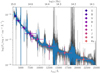 |
Fig. 2. Final fully-reduced and flux-calibrated optical-to-NIR X-shooter spectrum of the Crab pulsar. The seven individual spectra (Table 1) are plotted in black, whereas the blue line shows their average. As can be seen, all the spectra overlap even though obtained at different occasions. The spectra have been corrected for extinction as discussed in the text. The circles are photometric AB magnitudes from Sandberg & Sollerman (2009). |
The spectra of the pulsar, the flux standards, and telluric standard stars were reduced to bias-subtracted, flat-fielded, rectified, order-combined, flux- and wavelength-calibrated images for all three arms (UVB, VIS, and NIR) using the Reflex package and version 3.2 of the X-shooter pipeline (Modigliani et al. 2010). The standard stars and the telluric standards were both extracted by the ESO pipeline, in which an aperture the size of the nodding window, centered on the 2D-spectrum is used for standard extraction. For the extraction of the object spectra, we followed the data reduction steps outlined in Selsing et al. (2019), including the recalibration of both the wavelength solution and the application of a slit-loss correction. The wavelength solution is refined by cross-correlating the sky spectrum with a synthetic sky spectrum generated using the ESO Skycalc tool (Noll et al. 2012; Jones et al. 2013). After refinement of the wavelength solution, the spectra are corrected for barycentric motion. The slit-loss correction is estimated using the average DIMM seeing (V-band seeing at zenith, measured on the mountain, Sarazin & Roddier 1990) across the spectral integration window for each of the observations. The DIMM seeing is further corrected for the average airmass of the observation. Using the wavelength dependence of seeing (Boyd 1978), we can evaluate the effective seeing, at each wavelength bin. We synthetize a 2D-moffat profile, using the seeing at each wavelength, and the size of the spectroscopic slit is integrated over, yielding the throughput at each wavelength sampling of the spectrum. This can then be used to correct for the slit losses. The nightly ESO flux standard was observed with a wider slit (5 arcsec) than used for the object spectra (Table 1), therefore slit losses do not affect the flux standard observations. The telluric standard star observations were carried out using the same observational setup as the science observations, however because the absolute scaling of these are not important, we did not correct these for slit losses.
The telluric transmission spectra are found by fitting the telluric standard stars with a model atmosphere, using MolecFit (Smette et al. 2015). The science spectra are then corrected for the telluric transmission, by dividing by the atmospheric transmission for both the flux and error spectra. In this way, the error in the regions most affected by telluric absorption is increased, which ensures that a weighted fitting procedure correctly down-weight such regions.
To allow future assessments of the systematics of the reduction, for example the accuracy of telluric corrections and merging of spectral orders, we also make the flux-calibrated version of the spectrum from the spectrophotometric standard star GD 71 available at WISeREP (Yaron & Gal-Yam 2012), together with the final reduction of the pulsar spectra.
The resolution of each of the individual observations are found by fitting a series of unresolved telluric absorption lines with Voigt profiles. In more than half of the observations, the seeing is better than the slit widths and thus the actual spectral resolution is better than the nominal one. The nominal spectral resolutions are 55, 34 and 50 km s−1 in the three arms, respectively. In the best case, the fifth spectrum taken (Table 1), the seeing is only  , for which we derive an effective delivered resolution of 19 km s−1 in the VIS arm and 45 km s−1 in the NIR arm. There are no telluric lines in the UVB arm, but assuming that the average relative improvement in the resolution is the same would give 38 km s−1 in the UVB arm.
3. Spectral analysis
The individual spectra (Table 1) were reduced independently and exhibit small differences in the absolute flux scaling, with excellent agreement in the spectral slope (Fig. 2). To assess the agreement in the absolute flux level, we measure the flux density in a small region (∼50 Å wide) around 7000 Å. We measure 2.00 ± 0.158 × 10⁻¹⁵ erg s−1 cm−2 Å−1, where the error is the standard deviation of the flux densites. We scale all spectra to the single spectrum that minimizes the difference between the observed spectra and the measured photometry from Sandberg & Sollerman (2009), see Fig. 2. This error is also a measure of the precision of the absolute flux calibration, which suggests that the absolute scaling of the flux calibration is consistent to within 8%. This is in agreement with the accuracy reported by ESO3. This exercise shows that the variations due to seeing, airmass and use of different spectrophotometric standard stars were small, after the corrections described in the previous section are employed.
After the spectra have been calibrated and rescaled, we combine them using a inverse variance weighting scheme with the errors added in quadrature. To correct for the Milky Way extinction, we used a color excess of E(B − V)MW = 0.52 mag (Sollerman et al. 2000), and a standard (RV = 3.1) reddening law from Fitzpatrick & Massa (2007). We use a Python implementation of the reddening laws4.
In Fig. 2, we compare the individual spectra, overlaid with the combined one, with previously published photometry in this wavelength range from Sandberg & Sollerman (2009). We did not further scale the spectra, nor the photometry, and the two types of measurement are consistent within the errors across the entire wavelength coverage. This gives credibility to both the absolute flux scaling and to the shape across the spectral coverage of X-shooter. There are pros and cons with all these data, as discussed in Sect. 4, but the overall match is excellent.
In Fig. 3 we plot the data in log Fν versus log ν as is commonly done in the pulsar literature. In this figure we have also included the NUV HST data from Sollerman et al. (2000). The details of these data can be found in that paper, but we mention that we have now also uploaded this spectrum to WISeREP. The agreement between the slope and absolute flux scaling between the X-shooter spectra and the NUV HST data additionally supports the validity of the absolute flux calibration.
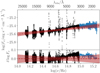 |
Fig. 3. Combined X-shooter spectrum in log-log space in black together with the best fit power-law in dashed red. This figure also includes the near-ultraviolet (NUV) HST spectrum from Sollerman et al. (2000) in blue. In the fit we have only included the X-shooter spectrum and removed some of the regions where the atmospheric transmission is low, as indicated in the plot. The spectral index is αν = 0.16 ± 0.07 as shown by the dashed line, where the red region encompasses 68% of the probability mass of the slope uncertainty, normalized at 7000 Å. Bottom panel: zooms in on the residuals between the best fit line and the observed data. |
We estimate the spectral index of the Crab pulsar, by fitting a power law to the full spectral range of X-shooter. In this part, care was taken to assess which parts of the spectra were reliable. All fits used the propagated errors from the reduction pipeline as weights, but we furthermore excluded a few wavelength ranges, like the strong telluric bands between the JHK bands in the NIR, and also the first order in the J band where the merging with the VIS arm was poor.
We fit for the spectral index in each individual spectrum (Table 1). The best fit parameters of the power law for each individual spectrum and the associated errors on the best fit values are found by sampling the posterior probability distributions of the parameters, assuming flat priors on all parameters. We use LMFIT (Newville et al. 2016) for the fitting implementation, which runs emcee (Foreman-Mackey et al. 2013) to carry out the sampling of the posterior probability distribution. We initiate 10 samplers, each sampling for 5000 steps, but discard the first 500 steps as a burn-in phase of the MCMC chains. We use the median of the marginalized posterior probability distribution as the best-fit values, and the 16th and 84th percentiles as the uncertainties.
The individual slopes are then averaged, with the statistical uncertainties from the fits propagated. The best fit power law provides a spectral index of αν = 0.16 ± 0.07. The formal error on the individual linear fits is merely 0.001. To properly assess the systematics, we have fit power-laws to all the seven extracted spectra, and the rms of these provided spectral indices is 0.065. We add in quadrature the statistical errors from the fits and the standard deviation between the individual best fit slopes to propagate the error on the derived spectral index, and the error on the slope is here thus dominated by the variation between the individual spectra.
4. Caveats
Obtaining the correct and precise spectral index for the Crab pulsar is a challenge, even if we now have a spectrum of this 16.5 mag source with an 8m telescope. The ideal pulsar spectrum should be multi-wavelength, phase-resolved, high-resolution, background subtracted, simultaneous and properly flux calibrated. None of the efforts performed so far achieve all of these. We briefly discuss some of these caveats below.
4.1. Simultaneous and multi-wavelength
Most of the spectra in the literature cover only a fairly small spectral window in the optical, typically 4000–8000 Å. This range is rather limited when trying to assess the full spectral energy distribution from the ultraviolet to the infrared, or for many pulsars even extending from gamma-rays to radio (e.g., Kuiper et al. 2001).
Moreover, as limited spectral regions are patched together to construct the entire SED of the pulsar, there is the risk that observations obtained at different occasions are not easily matched. There is both the observational challenge in merging datasets from different instrumentation and observing conditions (for example seeing, airmass). For the Crab pulsar there is also the notion that the object itself may be intrinsically varying, both on the long time scales of secular evolution (Sandberg & Sollerman 2009) and on the variable background in terms of wisps and knots (Hester et al. 1995; Melatos et al. 2005; Rudy et al. 2015).
Our X-shooter spectrum is a step in the right direction, affording a wide wavelength range at the same occasions. However, with the present spatial resolution we can not guarantee that we are not probing the inner knot, where the importance is larger toward the reddest wavelengths (Sandberg & Sollerman 2009). What we can see from Fig. 2, however, is that the mis-match is not severe, given that all seven of our X-shooter spectra overlap nicely with previous photometric measurements.
4.2. Phase-resolved and high spatial resolution for background subtraction
With X-shooter, we can only aim at the integrated spectrum of the pulsar. Other kind of instrumentation is needed to phase-resolve the spectrum into the different components, as done for example by Sollerman et al. (2000) and Fordham et al. (2002).
This may not be a problem per se, but phase-resolved data may allow better background subtraction. Our data, even if obtained at sub-arcsecond seeing, may well be influenced by the nearby knot and other nebular structures. In fact, in nodding on the slit we are always within the nebula (which is very large on the sky at 6′×6′). Perfect background subtraction is therefore difficult in our data, even if the pulsar itself clearly dominates the signal.
4.3. Flux-calibration
In the set-up and execution of this project we made sure that a special spectrophotometric standard star GD 71 was co-observed with the pulsar, in order to allow assessing how good the overall relative flux-calibration is. Medium-resolution spectrographs like X-shooter are seldom designed to perform accurate flux-calibration, so this is also partly an investigation into how well this can be achieved, following previous such efforts (see e.g., Moehler et al. 2014; Pita et al. 2014). We present a short investigation of the flux-calibration accuracy of GD 71 in Appendix A. We have done as good as we can with flux-calibration of the spectrum – given the caveats listed above. The end result is a good signal-to-noise spectrum all across the UV-NIR wavelengths at medium resolution. However, there will always be room for improvements, and the deviations that we highlight in the bottom panel of Fig. 3 clearly includes a number of effects, including uncertainties in order overlap, imperfections from telluric corrections, absorption lines and DIBs as discussed in the next section as well as the caveats discussed above. This must be appreciated if discussing them in terms of pulsar physics.
5. Discussion
The theoretical discussion in Björnsson et al. (2010) highlighted that the main question regarding αν is whether or not it is consistent with a value of 1/3. This is the highest possible value for optically thin incoherent synchrotron radiation as the emission mechanism. They related this to both the electron distribution cut-off and to the magnetic field in the emission region. We here estimate αν = 0.16 ± 0.07 and this therefore remains completely consistent with a simple synchrotron radiation process. We see no strong evidence for a change in the slope at NIR wavelengths, as was previously discussed in the context of synchrotron self-absorption (O’Connor et al. 2005). In this sense, we confirm previous studies of the optical-NIR spectral index of the Crab pulsar, but with new confidence given the simultaneous and systematic multiwavelength approach. There is also room for improvement as mention in the previous section. Overall, the single power-law (PL) is not a prefect fit to the X-shooter spectrum, as emphasized in the residual panel of Fig. 3. A fit allowing a broken PL would in fact be formally preferred (Akaike Information Criteria; see Akaike 1974) but is also not convincing. The best fit two-component PL would have α1 = 0.03 ± 0.02 and α2 = 0.21 ± 0.04 with the break at log(νbreak) = 14.5 ± 0.1. Here, the spectral index in the redder region (α1) is flatter, which is the opposite to an infrared roll-over as suggested by O’Connor et al. (2005). We note in passing that their synchrotron self-absorption scenario for the Crab pulsar also implied a low NIR flux for the pulsar in supernova remnant (SNR) 0540−69.3, something that later observations did not confirm (Mignani et al. 2012). The somewhat steeper slope in the blue (α2) would overshoot the data in the NUV regime, instead of underpredicting it as for the single PL. For other optical pulsars, there have been discussions on broken power-law spectra, but the quality of the data (see e.g., Mignani et al. 2007, their Fig. 4) and the interpretation is unclear, so we do not discuss this further here.
6. Additional science
Flux calibration of the pulsar spectrum was the overall aim of this observational campaign. In this section we mention a few other results that can be deduced from the data, although we emphasize that the observations were not set up to optimize this kind of science. We briefly mention searching for absorption lines associated to the pulsar, interstellar medium or the supernova ejecta. We also detect a large number of emission lines from the ejecta filaments close to the pulsar. In particular, some of the NIR emission lines that we detect with the short slit centered on the pulsar have, to our knowledge, not been reported before from the Crab nebula. All data are available in the ESO archive if future projects want to make further use of these observations.
6.1. Cyclotron lines and diffuse interstellar bands
The full coverage high signal-to-noise spectrum allows us to search, for example, after potential cyclotron lines. The occurrence of such lines in pulsar spectra were proposed by for example Romani (2000) and putatively detected in the first modern high-quality spectrum of the Crab pulsar (Nasuti et al. 1996). However, subsequent observations did not detect these features (Sollerman et al. 2000). Beskin & Neustroev (2001) also reported non-detections of the particular feature, but cautioned – given similar claims for the Geminga – that the Crab pulsar cyclotron lines could be time-dependent.
We searched our spectra for any outstanding broad absorption or emission line. Again, no support for the putative cyclotron lines were detected. In particular, the region around 6000 Å, where Nasuti et al. (1996) tentatively detected a broad feature has high signal-to-noise but no sign of a broad feature in our spectrum.
On the other hand, we do detect a number of DIBs. Again, the combined spectrum is not ideal for a deep and systematic search for such features, given the contamination of filament emission-line background residuals, but on inspection we could indeed detect most of the stronger DIBs (Herbig 1995; Sollerman et al. 2005). We see for example a broad feature at 4430 Å with an equivalent width (EW) of 1.1 Å and a full width half maximum (FWHM) of 20 Å as measured using IRAF splot. This is one of the strongest DIBs in the list of Herbig (1995). Since carefully searching for DIBs is somewhat out of the scope for this paper, we simply went through the list of DIBs from Sollerman et al. (2005), and tabulate the ones we detected in Table 2. There is room for improvement in identifying more DIBs in these spectra. It could also be of interest to correlate the strengths of the DIBs in this line-of-sight since the extinction is quite high and well characterized (Sollerman et al. 2000).
Diffuse interstellar bands toward the Crab pulsar.
6.2. Emission lines from the nebula
Our pulsar exposures also include emission from the nebular filaments. In the UVB-VIS arms we see a multitude of lines with complex kinematics. Of course, emission line studies of the Crab nebula have been performed for decades, and the central region probed with our short slit is not where the very strongest emission in the Crab nebula resides. We can measure for example a maximum velocity of [O II] λλ3727, 3729 of 1287 km s−1 (blueshifted) and 1046 km s−1 (redshifted). Similarly, for the strong [O III] λ4959 we get 1402 and 1611 km s−1, respectively, and Hα also gives two shells with ±1400 km s−1.
This is all in accordance with the ejecta velocities previously reported in the literature for the Crab nebula. Apart from hydrogen lines we detect for example; He I λλ3889, 4026, 4471, 5876, 6678, 7065, He II λ4686, [C I] λλ9824, 9850, [N II] λλ 6548,6583, [Ni II] λ7377, [Ne III] λλ3869, 3968, [Ar III] λ7136, [S II] λλ6717, 6731, [S III] λλ9069, 9531, [O I] λλ6300, 6364, [O I] λ7772, [O II] λλ3727, 3729 and λλ7319, 7320, 7330, as well as [O III] λλ4363, 4959, 5007.
Since the optical emission lines have been well studied, we focus here instead on the NIR part of the spectrum. Surprisingly few NIR spectroscopic studies of the Crab nebula exist, and for many years the most comprehensive study (Graham et al. 1990) barely detected the strongest [Fe II], and molecular H2 lines. More recently, Richardson et al. (2013) discussed the NIR spectroscopic observations (K band) of Loh et al. (2012) which mention only observations of H I and H2 emission from some strong knots. There has been revived interest in the infrared community on the Crab nebula, also in trying to understand the dust mass from modeling (e.g., Temim & Dwek 2013; Owen & Barlow 2015).
Clearly, there are a number of disadvantages with our set-up, which was not optimized to search for emission lines. First of all, the X-shooter slit is only 11 arcsec long, and thus covers a very small part of the nebula – the very inner part that is mostly synchrotron dominated (Fig. 1). Additionally, the many exposures covered different regions due to the fixation at parallactic angle. Finally, the nodding was done within the nebula, so proper sky subtraction would also remove any uniform nebular emission lines.
Nevertheless, given the apparent lack of Crab nebula NIR emission lines reported in the literature, we have tabulated a number of the detected lines in Table 3. We did this by searching through the 2D image for one of the obtained OBs (no. 6), and tabulated the most conspicuous lines. The spectra are available for further studies. Apart from [Fe II] 1.64 μm which was detected by Graham et al. (1990) and He I 2.1 μm which was seen by Loh et al. (2012), we also detect for example [S II], [P II] as well as a number of additional iron lines. Phosphorus was also recently detected in Cas A (Koo et al. 2013), where they interpreted the high abundance as evidence for stellar nucleosynthesis. We identify all the six lines that Koo et al. found in Cas A also in our Crab spectra. It is obvious that a systematic approach targeting some of the brighter knots in the Crab Nebula with X-shooter would deliver a very rich emission line spectrum for nebular diagnostics.
Noticeable emission lines in the NIR.
6.3. Absorption lines
Finally, we also searched for absorption lines from the ISM and the nebula itself, using the pulsar as a background source. This has been suggested as a way of probing the possible fast shell around the Nebula (c.f., Lundqvist et al. 1986; Sollerman et al. 2000; Tziamtzis et al. 2009).
We scanned through both the combined pulsar spectrum, as well as the spectrum from OB6, in order to search for absorption lines. As displayed in Fig. 4, we clearly detect, for example, Ca II λλ3934,3968 in absorption at about rest wavelength. The lines are very narrow, and unresolved at the resolution of X-shooter. Tappe (2004) used VLT/UVES to resolve several ISM absorption components, and derived interstellar column densities, Ncol (in units of cm−2), of Ca II, Na I and K I to be log(Ncol) = 13.03 ± 0.11, 13.36 ± 0.46 and 11.84 ± 0.03, respectively. Those numbers can be used, in combination with our measured equivalent widths of several DIBs, to relate extinction, DIB strengths and interstellar absorption lines.
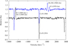 |
Fig. 4. Spectra (in velocity units) around Ca II λλ3934,3968. The spectrum in black centers on Ca II λ3934, whereas the spectrum in blue is centered on Ca II λ3968 and has been shifted +0.2 in relative flux units for clarity. The narrow, albeit unresolved, absorption close to zero velocity is interstellar absorption. No Ca II absorption originating in the Crab Nebula can be identified. Emission lines from the nebula (all from the nebula’s far side) have been marked. |
Figure 4 shows no hint of Ca II λ3934 absorption in the velocity interval −2000 km s−1 < v < 0 km s−1, and particularly none at ∼ − 1700 km s−1, as was evidenced for C IV λλ1548, 1551 (Sollerman et al. 2000). Our deep X-shooter spectra can thus rule out similar Ca II λ3934 absorption with much greater confidence than the data discussed by Lundqvist & Tziamtzis (2012), which is obvious from a comparison between Fig. 4, and their Fig. 6. Any calcium present in the near side of the Crab Nebula must be ionized to Ca III, or higher.
7. Conclusions
To summarize, we have used the X-shooter three-arm echelle spectrograph on VLT to obtain a UV-NIR spectrum of the Crab pulsar. Summing seven individual but mutually consistent spectra we derive a power-law spectral index of αν = 0.16 ± 0.07 for the entire regime, which is consistent with previous measurements, and fits with the NUV HST spectrum. Although not free of systematics, we consider this the best effort to date to characterize the pulsar SED in this regime, and the result appears to be consistent with synchrotron radiation with little evidence for self-absorption in the NIR.
In addition to the pulsar spectrum, we also highlight a few other aspects of these data. We detected a number of diffuse interstellar bands which have previously not been reported toward the Crab, and also several NIR emission lines, including phosphorus, that to our knowledge have not been previously discussed in the Crab literature. All data are now publicly available, and more investigations are encouraged.
Program 092.D-0260, P.I. Sollerman.
Program 096.D-0847, P.I. Nyholm.
Acknowledgments
The authors would like to acknowledge Claes-Ingvar Björnsson, Yura Shibanov and Bo Milvang-Jensen for early discussions on this project. This work is based on observations collected at the European Organisation for Astronomical Research in the Southern Hemisphere. The Oskar Klein Centre is funded by the Swedish Research Council. Thanks also to the anonymous referee who asked us to look into the broken power-law option.
References
- Akaike, H. 1974, IEEE Trans. Autom. Control, 19, 716 [NASA ADS] [CrossRef] [MathSciNet] [Google Scholar]
- Beskin, G. M., & Neustroev, V. V. 2001, A&A, 374, 584 [NASA ADS] [CrossRef] [EDP Sciences] [Google Scholar]
- Björnsson, C.-I., Sandberg, A., & Sollerman, J. 2010, A&A, 516, A65 [NASA ADS] [CrossRef] [EDP Sciences] [Google Scholar]
- Boyd, R. W. 1978, J. Opt. Soc. Am., 68, 877 [NASA ADS] [CrossRef] [Google Scholar]
- Bühler, R., & Blandford, R. 2014, Rep. Prog. Phys., 77, 066901 [NASA ADS] [CrossRef] [PubMed] [Google Scholar]
- Carramiñana, A., Čadež, A., & Zwitter, T. 2000, ApJ, 542, 974 [NASA ADS] [CrossRef] [Google Scholar]
- Crusius-Wätzel, A. R., Kunzl, T., & Lesch, H. 2001, ApJ, 546, 401 [NASA ADS] [CrossRef] [Google Scholar]
- Fitzpatrick, E. L., & Massa, D. 2007, ApJ, 663, 320 [NASA ADS] [CrossRef] [EDP Sciences] [Google Scholar]
- Fordham, J. L. A., Vranesevic, N., Carramiñana, A., et al. 2002, ApJ, 581, 485 [NASA ADS] [CrossRef] [Google Scholar]
- Foreman-Mackey, D., Hogg, D. W., Lang, D., & Goodman, J. 2013, PASP, 125, 306 [CrossRef] [Google Scholar]
- Galazutdinov, G. A., Musaev, F. A., Krełowski, J., & Walker, G. A. H. 2000, PASP, 112, 648 [NASA ADS] [CrossRef] [Google Scholar]
- Graham, J. R., Wright, G. S., & Longmore, A. J. 1990, ApJ, 352, 172 [NASA ADS] [CrossRef] [Google Scholar]
- Herbig, G. H. 1995, ARA&A, 33, 19 [NASA ADS] [CrossRef] [Google Scholar]
- Hester, J. J. 2008, ARA&A, 46, 127 [Google Scholar]
- Hester, J. J., Scowen, P. A., Sankrit, R., et al. 1995, ApJ, 448, 240 [NASA ADS] [CrossRef] [Google Scholar]
- Jones, A., Noll, S., Kausch, W., Szyszka, C., & Kimeswenger, S. 2013, A&A, 560, A91 [NASA ADS] [CrossRef] [EDP Sciences] [Google Scholar]
- Koo, B.-C., Lee, Y.-H., Moon, D.-S., Yoon, S.-C., & Raymond, J. C. 2013, Science, 342, 1346 [NASA ADS] [CrossRef] [PubMed] [Google Scholar]
- Kuiper, L., Hermsen, W., Cusumano, G., et al. 2001, A&A, 378, 918 [NASA ADS] [CrossRef] [EDP Sciences] [Google Scholar]
- Loh, E. D., Baldwin, J. A., Ferland, G. J., et al. 2012, MNRAS, 421, 789 [NASA ADS] [Google Scholar]
- Lundqvist, P., & Tziamtzis, A. 2012, MNRAS, 423, 1571 [NASA ADS] [CrossRef] [Google Scholar]
- Lundqvist, P., Fransson, C., & Chevalier, R. A. 1986, A&A, 162, L6 [NASA ADS] [Google Scholar]
- Martin, C., Halpern, J. P., & Schiminovich, D. 1998, ApJ, 494, L211 [NASA ADS] [CrossRef] [Google Scholar]
- Massaro, E., Campana, R., Cusumano, G., & Mineo, T. 2006, A&A, 459, 859 [NASA ADS] [CrossRef] [EDP Sciences] [Google Scholar]
- Melatos, A., Scheltus, D., Whiting, M. T., et al. 2005, ApJ, 633, 931 [NASA ADS] [CrossRef] [Google Scholar]
- Mignani, R. P., Zharikov, S., & Caraveo, P. A. 2007, A&A, 473, 891 [NASA ADS] [CrossRef] [EDP Sciences] [Google Scholar]
- Mignani, R. P., De Luca, A., Hummel, W., et al. 2012, A&A, 544, A100 [NASA ADS] [CrossRef] [EDP Sciences] [Google Scholar]
- Modigliani, A., Goldoni, P., Royer, F., et al. 2010, in Observatory Operations: Strategies, Processes, and Systems III, Proc. SPIE, 7737, 773728 [CrossRef] [Google Scholar]
- Moehler, S., Modigliani, A., Freudling, W., et al. 2014, A&A, 568, A9 [NASA ADS] [CrossRef] [EDP Sciences] [Google Scholar]
- Nasuti, F. P., Mignani, R., Caraveo, P. A., & Bignami, G. F. 1996, A&A, 314, 849 [NASA ADS] [Google Scholar]
- Newville, M., Stensitzki, T., Allen, D. B., et al. 2016, Astrophysics Source Code Library [record ascl:1606.014] [Google Scholar]
- Noll, S., Kausch, W., Barden, M., et al. 2012, A&A, 543, A92 [NASA ADS] [CrossRef] [EDP Sciences] [Google Scholar]
- O’Connor, P., Golden, A., & Shearer, A. 2005, ApJ, 631, 471 [NASA ADS] [CrossRef] [Google Scholar]
- Oke, J. B. 1969, ApJ, 156, L49 [NASA ADS] [CrossRef] [Google Scholar]
- Owen, P. J., & Barlow, M. J. 2015, ApJ, 801, 141 [NASA ADS] [CrossRef] [Google Scholar]
- Pita, S., Goldoni, P., Boisson, C., et al. 2014, A&A, 565, A12 [NASA ADS] [CrossRef] [EDP Sciences] [Google Scholar]
- Richardson, C. T., Baldwin, J. A., Ferland, G. J., et al. 2013, MNRAS, 430, 1257 [NASA ADS] [CrossRef] [Google Scholar]
- Romani, R. W. 2000, in Highly Energetic Physical Processes and Mechanisms for Emission from Astrophysical Plasmas, eds. P. C. H. Martens, S. Tsuruta, & M. A. Weber, IAU Symp., 195, 95 [NASA ADS] [Google Scholar]
- Romani, R. W., Miller, A. J., Cabrera, B., Nam, S. W., & Martinis, J. M. 2001, ApJ, 563, 221 [NASA ADS] [CrossRef] [Google Scholar]
- Rudy, A., Horns, D., DeLuca, A., et al. 2015, ApJ, 811, 24 [NASA ADS] [CrossRef] [Google Scholar]
- Sandberg, A., & Sollerman, J. 2009, A&A, 504, 525 [NASA ADS] [CrossRef] [EDP Sciences] [Google Scholar]
- Sarazin, M., & Roddier, F. 1990, A&A, 227, 294 [NASA ADS] [Google Scholar]
- Selsing, J., Malesani, D., Goldoni, P., et al. 2019, A&A, 623, A92 [NASA ADS] [CrossRef] [EDP Sciences] [Google Scholar]
- Serafimovich, N. I., Shibanov, Y. A., Lundqvist, P., & Sollerman, J. 2004, A&A, 425, 1041 [NASA ADS] [CrossRef] [EDP Sciences] [Google Scholar]
- Shearer, A., & Golden, A. 2002, in Neutron Stars, Pulsars, and Supernova Remnants, eds. W. Becker, H. Lesch, & J. Trümper, 44 [Google Scholar]
- Smette, A., Sana, H., Noll, S., et al. 2015, A&A, 576, A77 [NASA ADS] [CrossRef] [EDP Sciences] [Google Scholar]
- Sollerman, J. 2003, A&A, 406, 639 [NASA ADS] [CrossRef] [EDP Sciences] [Google Scholar]
- Sollerman, J., Lundqvist, P., Lindler, D., et al. 2000, ApJ, 537, 861 [NASA ADS] [CrossRef] [Google Scholar]
- Sollerman, J., Cox, N., Mattila, S., et al. 2005, A&A, 429, 559 [NASA ADS] [CrossRef] [EDP Sciences] [Google Scholar]
- Tappe, A. 2004, PhD Thesis, PhD Dissertation, 2004. 138 pages; Sweden: Chalmers Tekniska Hogskola (Sweden); 2004. Publication Number: AAT C819472. DAI-C 66/02, p. 432, Summer 2005 [Google Scholar]
- Temim, T., & Dwek, E. 2013, ApJ, 774, 8 [NASA ADS] [CrossRef] [Google Scholar]
- Tziamtzis, A., Schirmer, M., Lundqvist, P., & Sollerman, J. 2009, A&A, 497, 167 [NASA ADS] [CrossRef] [EDP Sciences] [Google Scholar]
- Vernet, J., Kerber, F., Saitta, F., et al. 2008, in Observatory Operations: Strategies, Processes, and Systems II, Proc. SPIE, 7016, 70161G [CrossRef] [Google Scholar]
- Vernet, J., Dekker, H., D’Odorico, S., et al. 2011, A&A, 536, A105 [NASA ADS] [CrossRef] [EDP Sciences] [Google Scholar]
- Yaron, O., & Gal-Yam, A. 2012, PASP, 124, 668 [NASA ADS] [CrossRef] [Google Scholar]
- Zharikov, S., Mennickent, R. E., Shibanov, Y., & Komarova, V. 2007, Astrophys. Space Sci., 308, 545 [NASA ADS] [CrossRef] [Google Scholar]
Appendix A: Flux accuracy
As also described in the main text, we observed the spectrophotometric standard star, GD 71, using the exact same spectroscopic set-up as for the Crab pulsar observations, including exposure time, readout mode and slit widths (Table 1). The observations of GD 71 were carried out between two consecutive epochs of Crab pulsar X-shooter observations and the comparison between our observed spectra of GD 71 and the model spectra presented in Moehler et al. (2014) should thus represent the relative flux calibration accuracy of the Crab pulsar observations. We show this in Fig. A.1 which demonstrates an overall relative flux accuracy of ∼ ± 3%. We can also see some structure in the ratio, which includes differences between the real stellar spectrum and the model, but also artifacts like echelle order overlaps and residuals from telluric corrections. Again, the overall effect of these are at the percent level, which should be remembered when interpreting wiggles in the pulsar spectrum itself.
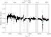 |
Fig. A.1. Comparison of here we compare the flux-calibrated spectrum from the observations we made of the spectrophotometric standardstar GD 71 using the same setup as for the Crab pulsar with a model spectrum of the same star. We have plotted the ratio between these observations, and the blue line is a best fit power-law which shows a slight slope which could mean a relative error in flux calibration of ±3% over the entire wavelength region of X-shooter. |
All Tables
All Figures
|
Fig. 1. An acquisition image of Crab pulsar and neighborhood from our X-shooter observations. The position angles provided in Table 1 are overlaid to show where the observations were obtained. The widths of the slits shown are 0 |
| In the text | |
|
Fig. 2. Final fully-reduced and flux-calibrated optical-to-NIR X-shooter spectrum of the Crab pulsar. The seven individual spectra (Table 1) are plotted in black, whereas the blue line shows their average. As can be seen, all the spectra overlap even though obtained at different occasions. The spectra have been corrected for extinction as discussed in the text. The circles are photometric AB magnitudes from Sandberg & Sollerman (2009). |
| In the text | |
|
Fig. 3. Combined X-shooter spectrum in log-log space in black together with the best fit power-law in dashed red. This figure also includes the near-ultraviolet (NUV) HST spectrum from Sollerman et al. (2000) in blue. In the fit we have only included the X-shooter spectrum and removed some of the regions where the atmospheric transmission is low, as indicated in the plot. The spectral index is αν = 0.16 ± 0.07 as shown by the dashed line, where the red region encompasses 68% of the probability mass of the slope uncertainty, normalized at 7000 Å. Bottom panel: zooms in on the residuals between the best fit line and the observed data. |
| In the text | |
|
Fig. 4. Spectra (in velocity units) around Ca II λλ3934,3968. The spectrum in black centers on Ca II λ3934, whereas the spectrum in blue is centered on Ca II λ3968 and has been shifted +0.2 in relative flux units for clarity. The narrow, albeit unresolved, absorption close to zero velocity is interstellar absorption. No Ca II absorption originating in the Crab Nebula can be identified. Emission lines from the nebula (all from the nebula’s far side) have been marked. |
| In the text | |
|
Fig. A.1. Comparison of here we compare the flux-calibrated spectrum from the observations we made of the spectrophotometric standardstar GD 71 using the same setup as for the Crab pulsar with a model spectrum of the same star. We have plotted the ratio between these observations, and the blue line is a best fit power-law which shows a slight slope which could mean a relative error in flux calibration of ±3% over the entire wavelength region of X-shooter. |
| In the text | |
Current usage metrics show cumulative count of Article Views (full-text article views including HTML views, PDF and ePub downloads, according to the available data) and Abstracts Views on Vision4Press platform.
Data correspond to usage on the plateform after 2015. The current usage metrics is available 48-96 hours after online publication and is updated daily on week days.
Initial download of the metrics may take a while.