| Issue |
A&A
Volume 629, September 2019
|
|
|---|---|---|
| Article Number | A78 | |
| Number of page(s) | 10 | |
| Section | Interstellar and circumstellar matter | |
| DOI | https://doi.org/10.1051/0004-6361/201833820 | |
| Published online | 10 September 2019 | |
X-ray extinction from interstellar dust
Prospects of observing carbon, sulfur, and other trace elements
1
SRON, Netherlands Institute for Space Research,
Sorbonnelaan, 2,
3584
CA,
Utrecht, The Netherlands
e-mail: This email address is being protected from spambots. You need JavaScript enabled to view it.
2
Leiden Observatory, Leiden University,
PO Box 9513,
2300 RA Leiden, The Netherlands
3
Anton Pannekoek Institute, University of Amsterdam,
Postbus 94249,
1090 GE Amsterdam, The Netherlands
4
Academia Sinica Institute of Astronomy and Astrophysics, 11F of AS/NTU Astronomy-Mathematics Building,
No. 1, Section 4, Roosevelt Rd,
Taipei 10617, Taiwan, ROC
Received:
10
July
2018
Accepted:
5
June
2019
Abstract
Aims. We present a study on the prospects of observing carbon, sulfur, and other lower abundance elements (namely Al, Ca, Ti, and Ni) present in the interstellar medium using future X-ray instruments. We focus in particular on the detection and characterization of interstellar dust along the lines of sight.
Methods. We compared the simulated data with different sets of dust aggregates, either obtained from past literature or measured by us using the SOLEIL-LUCIA synchrotron beamline. Extinction by interstellar grains induces modulations of a given photolelectric edge, which can be in principle traced back to the chemistry of the absorbing grains. We simulated data of instruments with characteristics of resolution and sensitivity of the current Athena, XRISM, and Arcus concepts.
Results. In the relatively near future, the depletion and abundances of the elements under study will be determined with confidence. In the case of carbon and sulfur, the characterization of the chemistry of the absorbing dust will be also determined, depending on the dominant compound. For aluminum and calcium, despite the large depletion in the interstellar medium and the prominent dust absorption, in many cases the edge feature may not be changing significantly with the change of chemistry in the Al- or Ca-bearing compounds. The exinction signature of large grains may be detected and modeled, allowing a test on different grain size distributions for these elements. The low cosmic abundance of Ti and Ni will not allow us a detailed study of the edge features.
Key words: dust, extinction / X-rays: ISM / techniques: spectroscopic / X-rays: individuals: GX5-1 / X-rays: individuals: GX340+00 / X-rays: individuals: GX3+1
© ESO 2019
1 Introduction
Absorption and scattering in the X-ray band has proved a useful diagnostic of the properties of interstellar dust (ID). By virtue of broadband coverage, the X-ray band displays many photoelectric absorption edges caused by the mixture of gas and dust intervening along the line of sight toward bright background sources (Draine 2003; Hoffman & Draine 2016). Absorption by interstellar grains is detected as a result of the interaction between an incoming X-ray photon and the electrons inside the grain’s atoms. The multiple-generated photoelectron-waves interfere with each other both constructively and destructively. This interference pattern depends on the complexity of the chemical compound and the distance of the electrons from the nucleus. Each pattern is a fingerprint of a given material (Rehr & Albers 2000). The extinction cross section, the sum of the absorption and scattering cross section (e.g., Draine 2003; Corrales et al. 2016) in the X-ray band, provides, in principle, not only a direct estimate of the chemistry of the interstellar medium (ISM), but also information on the size distribution, crystallinity, and porosity of the intervening grains (Hoffman & Draine 2016; Zeegers et al. 2017; Rogantini et al. 2018).
Early studies already pointed out that absorption by the ISM has contributed to the shape of X-ray spectra (Schattenburg & Canizares 1986; Paerels et al. 2001; Juett et al. 2004). However, in recent years, the deep features of the Fe L, O K, and Si K edges have been recognized to be largely caused by dust absorption (e.g., Lee et al. 2002; Ueda et al. 2005; Schulz et al. 2016) and have been studied using the grating spectrometers on board the X-ray observatories Chandra and XMM-Newton. These studies made use of absorption profiles either taken from the literature (Costantini et al. 2012; Pinto et al. 2010, 2013; Valencic & Smith 2013) or obtained with dedicated synchrotron measurements (Lee et al. 2009; Zeegers et al. 2017, 2019).
Outside the energy band where the sensitivity and resolution of the current instruments is maximized, it is at this moment challenging to study ID. An example is given by the tentative study of the C K edge (Schneider & Schmitt 2010), which was severely hampered by various instrumental effects, although the carbon edge would formally be included in the energy range of Chandra-LETGS.
In this paper we investigate the prospective of observing and modeling the elements of the ID that have not yet been studied, which happen to fall in the 1.5–8.3 keV band (Al, S, Ca, Ti, Ni) and at E < 0.5 keV (carbon). For a discussion on how the features that can be currently studied (O K, Fe L Mg K, and Si K edges) will be viewed by future instruments, we refer to works such as Decourchelle et al. (2013) and Smith et al. (2016).
In Fig. 1 we show the abundance pattern of the photoelectric absorption edges of the elements (with atomic number A = 6–30) as a function of the X-ray energy. The empty diamonds denote the edges that have been already studied by current instruments unveiling the dust features: the O K and Fe L edges at 0.534 and 0.7 keV, respectively (Lee et al. 2009; Costantini et al. 2012; Pinto et al. 2010, 2013; Valencic & Smith 2013); and the Mg and Si-K edges at 1.3 and 1.84 keV, respectively (Zeegers et al. 2017, 2019, Rogantini et al., in prep.). The black triangles indicate the edges presented in this work. We present the Fe K edge, indicated with a light gray triangle in the figure, in a separate paper (Rogantini et al. 2018), but see also Lee & Ravel (2005). The middle panel shows the range of depletion, defined as the amount of dust overthe total amount of matter in the ISM (dust and gas) that is expected for a given element. The wide range of depletions for some elements is due to the different density environments where those are observed (e.g., Jenkins 2009).
In the bottom panel of Fig. 1 we show the energy range of present and future missions. The solid line highlights the region in which the instrument capabilities (resolution and effective area) are optimal to observe the dust absorption features. The Chandra and XMM-Newton observatories (both launched in 1999, Weisskopf 1999; Jansen et al. 2001) are still in operation. The grating spectrometer Arcus will cover the soft X-ray range (Table 1). It is a NASA mission currently in the study phase (Smith et al. 2016). The calorimeter on board the X-ray Imaging Spectroscopy Mission (XRISM; to be launched around 2021) is planned to have the same characteristics of that on board of the lost Hitomi satellite (Mitsuda et al. 2014). Finally, we show the energy coverage of the Athena calorimeter XIFU (Barret et al. 2016) to be launched in 2030. The calorimeters on board XRISM and Athena will be optimal to observe the higher energy dust features (Table 1).
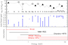 |
Fig. 1 Top panel: abundance pattern as a function of energy for the absorbing elements in the X-ray band. The K-edge energy is indicated, except from Fe, for which both the K and the L edges, at 7.1 and ~0.7 keV, respectively, can be studied. Abundances follow Lodders (2010) and they are expressed in terms of log (X/H)+12. In this frame, the abundance of hydrogen is 12. The open diamonds indicate the elements that are accessible by current instruments. The triangles indicate the relevant elements that will be accessible by future instruments to study dust. The black triangles indicate the subject of this work. Middle panel: range of depletions as reported by Jenkins (2009) for all elements, except C (Jenkins 2009; Whittet 2003), F (Snow et al. 2007), Na (Turner 1991), S (Gry & Jenkins 2017), K (Snow 1975), Ca (Crinklaw et al. 1994), Co (Federman et al. 1993), Al (Jenkins & Wallerstein 1996), and Ar (Sofia & Jenkins 1998). Bottom panel: energy range covered by present and future (red)mission. The solid line highlights the energy range for which the instruments capabilities are optimal for observing absorption by dust. |
Parameters of the instruments used in the simulations at the energy of the elements studied in this work.
2 Elements in this study
Carbon, oneof the major players in ID constitutes around 20% of the total depleted mass in the Galaxy (Whittet 2003). Its depletion covers a relatively narrow range of values (Fig. 1) showing that it is not a strong function of environmental density. It has been hypothesized that the majority of carbon should be locked in graphite grains, as a likely explanation for the 2175 Å emission feature (Draine 1989, 2003, and references therein). Graphite has been commonly adopted in ID models (e.g., Mathis et al. 1977). However, observational evidence pointed out that graphite cannot explain the variability of the 2175 Å feature (Fitzpatrick & Massa 2007). Furthermore, in analogy with the silicates, which are found to be amorphous, also graphite was deemed unlikely to survive in large quantities in the harsh environment of the ISM. Graphite should therefore face a natural process of amorphization (Compiègne et al. 2011).
The idea of carbon as a single and separate phase from the silicate population does not agree with a scenario of a constantly evolving and mixing medium (Jones et al. 2017). Hydrogenated amorphous carbon (HAC) may indeed coat the silicate grains, forming a single population (e.g., Duley et al. 1989) with different characteristics with respect to the environment in which they reside and depending on the particle size (e.g., Jones et al. 2017, and references therein). Polarization studies however have so far not confirmed this scenario. The carbon feature at 3.4 μm shows a negligible degree of polarization with respect to the silicate feature at 9.7μm, pointing to two distinct grain populations (Whittet 2011).
Finally, under special condition of high pressure, for instance in a shocked environment, graphite and amorphous carbon can turn into nano-diamonds, which can constitute as much as 5% of the amount of C in the ISM (Tielens et al. 1987), possibly with H and N inclusion (Van Kerckhoven et al. 2002; Bilalbegović et al. 2018). Diamonds of possible ISM origin have been found in meteorites (Lewis et al. 1987). An important carbon carrier are polycyclic aromatic hydrocarbons (PAH), large molecules (Ångstrom-sized) formed by carbon and hydrogen in a honeycomb structure. These molecules constitute up to about 10% of the carbon abundance (e.g., Tielens 2013). PAHs are very sensitive to ionizing radiation from far-ultraviolet to X-rays and they are easily destroyed near star formation sites at AU distance scale (e.g., Siebenmorgen & Krügel 2010), up to kiloparsec scale, for active galaxies (Voit 1992).
Apart from C, other constituents can be studied in detail by future generation telescopes. Sulfur in the dust phase seems to be absent from the diffuse ISM (Sembach & Savage 1996). However, a relative fast transition to a depletion approaching −1 dex is reported in dense media, such as molecular clouds (Joseph et al. 1986). In molecular clouds, sulfur can be included in aggregates such as H2S, SO2, OCS, SO, H2 CS, NS SiS, CS, HNCS CH3SH (Duley et al. 1980, and references therein) as well as other carbon-hydrogen bearing sulfates (e.g., Bilalbegović & Baranović 2015). Molecular reactions may also lead to sulfur aggregation into polymeric forms, such as S8 (e.g., Jiménez-Escobar & Muñoz Caro 2011). However, even integrating the contribution of all S-bearing molecules, the absolute abundance of sulfur in molecular clouds compared to the diffuse ISM abundance, with a ratio of ~ 10−8∕10−5, is inexplicably low (Wakelam & Herbst 2008). Inclusion into simple atomic sulfur or sulfur ices have been proposed to solve the missing-sulfur problem in molecular clouds (e.g., Vidal et al. 2017).
Sulfur in dust has also been detected near C-rich AGB stars, planetary nebulae (Hony et al. 2002), and protoplanetary disks (Keller et al. 2002), predominantly in form of troilite (FeS). Finally, sulfur is abundant in solid form in planetary systems bodies, such as interplanetary dust particles, meteorites, and comets (e.g., Wooden 2008, and references therein).
The presence of sulfur in dust form in the ISM has been suggested in association with glasses with embedded metal and sulfides (GEMS; Bradley 1994), where the FeS particles would be more concentrated on the surface of the glassy silicate. However, the majority of GEMS may well be of nebular origin, rather than the ISM (Keller & Messenger 2008). Sulfur in FeS, consistently of ISM origin, has been recorded in the data from the Stardust mission (Westphal et al. 2014). This evidence revitalizes the idea of the presence of sulfur in dust form in less dense environments of the ISM as well. The presence of strong UV radiation and cosmic rays has been thought to be the cause for the extreme sputtering of the highly volatile S, for example from GEMS surfaces. Recent experiments however put to the test this hypothesis (Keller et al. 2010), showing that UV bombardment has in fact little influence on sulfur stuck on a grain surface.
Aluminum, calcium, and titanium are extremely depleted in the ISM (Fig. 1). Ca and Ti also show a very similar depletion pattern as a function of gas density (Crinklaw et al. 1994). These two elements are found in gas only in tenuous environments, associated with warm inter cloud media in both the halo (Edgar & Savage 1989) and the disk of the Galaxy (Crinklaw et al. 1994). The depletion of Ti is severe, regardless of the environment, ranging between −1 and −3.1 dex (Welty & Crowther 2010). The ratio of column density between Ti II and Ca II, which is representative of the element neutral gas phase, is in general constant in the Galaxy (~0.4, Hunter et al. 2006). Al, Ca, and Ti have a similar condensation temperature (1400–1600 K, Field 1974); it has been hypothesized that because these molecules are the first to form in, for example, a stellar envelope or a supernova environment, they would form the core of complex dust grains with silicate and possibly ice mantles (e.g., Clayton 1978). This would provide a natural shield for these Al, Ca, and Ti-bearing compounds, preventing their destruction and ensuring a high depletion in the vast majority of the environments. Under the condition of thermodynamic equilibrium, aluminum first condenses in Al2 O3. From thereit may evolve into spinel (MgAl2O4) and eventually into a Ca and Al-bearing silicate. The latter are stable compounds, thanks to very high binding energies (Trivedi & Larimer 1981). Calcium is mostly locked in dust in silicates (e.g., CaMgSi2O6; Field 1974; Trivedi & Larimer 1981). Calcium carbonates, possibly formed in AGB stars envelopes (e.g., Kemper et al. 2002), are believed to be unstable and therefore Ca inclusion in silicates, which already form at high temperatures, are favored (Ferrarotti & Gail 2005). Titanium is produced by AGB stars mostly in the form of TiO2, which constitute a seed nucleus later included in the larger, coated grains (e.g., Ferrarotti & Gail 2006).
Nickel depletion is found to correlate with that of Fe for a variety of environments, from planetary nebulae (Delgado-Inglada et al. 2016)to diffuse interstellar clouds (Jenkins 2009). These two elements display a similar condensation temperature (1336 and 1354 K for Fe and Ni, respectively, Wasson 1985), which already points to a simultaneous inclusion into dust grains. However, it has been observed that in dense environments Ni is more depleted than Fe (e.g., Sembach & Savage 1996; Delgado-Inglada et al. 2016).
3 Extinction profiles
In this paper, we make use of literature values to infer the absorption absolute cross sections for all elements, except for Al (see below). Measurements of X-ray edges profiles are mostly carried out for industry and are rarely of interest for astronomical applications. For this reason, the sample selection is bound to be incomplete. The compounds used are listed in Table 2. We closely follow the method presented in Zeegers et al. (2017) and Rogantini et al. (2018) to obtain the extinction profiles to be confronted to the astronomical data. The laboratory data are transformed to transmission spectra and matched (via χ2 fitting) to tabulated transmission data of the same compound, where we assume an optically thin sample, as to mimic the conditions in the ISM. In doing this we only fit the pre- and post-edge of the tabulated data, leaving the edge energy as measured in the laboratory. The transmission tables are provided by the Center for X-ray Optics at Lawrence Berkeley National laboratory based on tabulated data by Henke et al. (1993). From the transmission spectra, the attenuation coefficient can be obtained and consequently we can obtain the imaginary part of the refractive index from this coefficient. The real part of the refractive index, m, is calculated via the Kramers-Kroning relations (Bohren 2010). The knowledge of m is needed to calculate the extinction cross section to involve both the effect of absorption and scattering. The extinction cross sections are calculated using Mie theory (Mie 1908; Wiscombe 1980) for C, Al, and S. We used instead the anomalous diffraction theory (ADT; van de Hulst 1957) for Ca, Ti and Ni. The anomalous diffraction theory can be used when the ratio x = 2πa∕λ ≫ 1, where a is the grain size and λ is the wavelength of the incident radiation. To obtain the extinction cross section for a range of dust grain radii, we assume the MRN size distribution (Mathis et al. 1977, and Sect. 4). Once the absolute cross section as a function of energy has been obtained, we implemented the extinction profiles in the already existing AMOL model in the fitting code SPEX (ver. 3.03, Kaastra et al. 1996). The AMOL model is an absorption model to be applied to the emitting continuum model of a source. It allows us to fit the X-ray edges for the column densities of a set of four dust compounds at a time (see also Zeegers et al. 2017). In real astronomical observations, the dust extinction feature always coexist with the gas feature of the corresponding element. The absolute energy of the edges of the gas phase may be reported in the literature at different energies, with discrepancies sometimes of few eV. In SPEX, the gas edge energies, for the elements in this work, are implemented following Verner et al. (1996). In this paper, we apply a shift to the laboratory data in order to consistently compare these data with the gas edge features as seen by SPEX. Discrepancies among different measurements and theoretical calculations may be found in the literature. High resolution X-ray spectroscopy will help determining the absolute energy scale of the edge (e.g., Gorczyca et al. 2013).
For Al, we made use of the laboratory data that we collected at the Line for Ultimate Charasterization by Imaging and Absorption (LUCIA) beamline at the Soleil synchrotron facility, which offers an energy resolution of ~0.25 eV. Both the samples, Al2 O3 and MgAl2O4, were commercially available from the Alfa-Aesar and Aldrich companies, respectively. The samples, in powder form, were pressed on thin indium foil and placed on a copper support, which was placed in a vacuum environment. The sample was then irradiated by an X-ray beam with tuneable energy. The X-ray fine structures were measured through fluorescence. At these soft X-ray energies, this method is more practical than the more intuitive method of measuring the transmission through the sample because for transmission measurements the samples have to be too thin to be easily handled. The fluorescent method to obtain the XAFS requires a correction for possible saturation. This correction was performed with the program routine FLUO (Stern et al. 1995). A full description of the procedure for the analysis of the data can be found in Zeegers et al. (2017).
Samples of ID analogs used in this work.
4 Simulations
We present the prospects of detecting absorption K edges relevant for dust studies using future missions (Fig. 1). The only instrument proposed for studying the soft X-ray energy band is, at this moment, the Arcus grating spectrometer1 (Smith et al. 2016). For the energy above ~2 keV, two microcalorimeters will provide an unprecedented resolution: Resolve and XIFU, onboard XRISM2 and Athena3 (Nandra et al. 2013), respectively. The effective area and resolving power of these three instruments at the energy of the features studied in this work are reported in Table 1. With the chosen exposure time we would obtain an associated error on the dust or gas column density of around 1% for C (Arcus) Al, S, and Ca (XIFU).
The simulations were carried out having in mind realistic scenarios in our Galaxy to prove the effective prospect of future instruments to measure physical parameters. We first simulated the data, considering the different instruments responses and including noise, assuming first that the photoelectric edge is only due to gas absorption. These simple simulations are confronted with models, folded with the appropriate response, which include an amount of gas set by the typical depletion found in the literature for a given element plus the contribution of a dust compound. We adopted the MRN dust size distribution in all cases. The MRN model offers a simple parameterization of the dust size distribution: n(a) ∝ a−3.5. It has been found to approximate at first order the conditions in our Galaxy for grain size between 0.025 and 0.25 μm. However, the exceptional depletion of Al and Ca, along with favorable observing conditions, also allowed us to test the detectability of a distribution in which the mass distribution is skewed toward larger grains (Draine & Fraisse 2009). This distribution has a size range of a = 0.02–1μm and has an average grain size of 0.6 μm. The observing conditions are favorable for these two elements first because the brightness of the sources with a favorable NH is often high, for example, low mass X-ray binaries (LMXBs) near the Galactic center (GC); second, the edges fall in a large effective-area region of the instrument.
Unless otherwise stated, we chose the maximum depletion allowed by previous studies (Table 1). This is a reasonable assumption in most cases. Indeed, for the photoelectric edge to be detected, a substantial column density is required. This also indicate a dense environment, where the depletion is large. In the following, we describe the conditions under which the simulations were performed for each element.
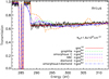 |
Fig. 2 Simulation in 500 ks of carbon K edge, using the Arcus grating, of an XRB in high state (F0.5−2 keV ~ 3 × 10⁻⁹ erg cm−2 s−1). The simulation considers different carbon species with a dust depletion of 60%. The two absorption lines belong to the atomic phase of C, namely C I. |
Carbon
The depletion of carbon has been optimistically assumed to be 0.6, but still implies a substantial role in gas absorption in the carbon edge. For this reason, although the edge feature itself can also be detected at relatively small column density (e.g., NH > 1020 cm−2), a much larger amount of matter is necessary to make the dust features evident. We simulated a column density of NH = 1.6 × 1021 cm−2 for a flux in the soft energy band of ~ 3 ×10⁻⁹ erg cm−2 s−1 (Fig. 2). We note that for this column density, the C I absorption lines from gas are already saturated (Fig. 2), therefore they cannot be used straightforwardly to measure depletion. Although this value for a column density is not uncommon for LMXBs, the source needs to be in an hypothetical high state to be well detected by an Arcus-like instrument as the effective area of such an instrument would fall rapidly at the carbon edge.
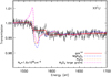 |
Fig. 3 Simulation in 300 ks of the aluminum K edge, using the XIFU calorimeter, of the bright XRB GX 3+1 (F2−10 keV ~ 3 × 10⁻⁹ erg cm−2 s−1). The dust depletion is 100%. The data have been binned for clarity. |
Aluminum
The cosmic abundance of Al is significantly less than the main ID components (Fig. 1). However, Al in the ISM is almost completely depleted onto dust. We simulated the contribution of Al2 O3 and MgAl2O4 and compared these with a theoretical pure gas absorption (Fig. 3). At ISM temperature Al, if it was totally in gas form, would be distributed between Al I and Al II. For this simulation we selected the bright LMXB (F2−10 keV ~ 3 × 10⁻⁹ erg cm−2 s−1) GX 3+1 whose spectral parameters where obtained from Chandra-HETGS data (obsid 16 492).
Sulfur
For the sulfur simulation, we selected GX 5-1, which is among the brightest LMXB in the Galaxy and has F2−10 keV ~ 2.5 × 10⁻⁸ erg cm−2 s−1. The hydrogen column density is about 3.4 ×1022 cm−2 (Zeegers et al. 2017). The depletion of sulfur is unknown in the diffuse ISM, but it has been estimated that could be up to ~46% (Fig. 1 and Gry & Jenkins 2017). We simulated a more conservative 30% depletion. Given the relatively low depletion of S, the XAFS features (Fig. A.1) would be less evident in the data (Fig. 4).
Calcium
The X-ray spectrum is only sensitive to calcium extinction if the intervening column density is sufficiently high. This is because of the relatively high energy position of the photoelectric edge. In Fig. 5 we simulated GX 340+00 (F2−10 keV ~ 1.3 × 10⁻⁸ erg cm−2 s−1) and has a column density of about NH ~ 6.9 × 1022 cm−2 that is obtained from HETG-Chandra data fitting (obsid 6632).
Titanium and nickel
For both these elements, we simulated an hypothetical source, for example near the GC, where the occurrence of high column density molecular clouds is also more frequent, which in outburst reaches a flux as high as GX 340+00 (Figs. 6 and 7). The column density must be sufficient to produce an edge-like modulation in the spectrum (NH ~ 1.3 × 1023 cm−2, Fig. A.2).
5 Discussion
5.1 Carbon
In the simulation we included gas and carbon forms that are believed to be most abundant (namely graphite, amorphous carbon, and HAC). While the difference between graphite and amorphous carbon is subtle, HAC has more distinctive features that may be more easily detected. The hydrogenation of carbon may point to either an environment protected from strong radiation or the presence of large grains, which are more resilient to radiation (Sect. 2).
For illustrative purposes, we also include diamonds (orange dashed line in Fig. 2) to show the departure of this form of carbon from the shape of, for example, graphite. However, in practice, diamonds are believed to constitute no more than 5% of the carbon (Tielens 2001). Its realistic inclusion would be nondetectable (dash-dotted blue line in figure). The same negligible effect may be produced by PAH, which we did not include in our simulation. The total amount along a line of sight is relatively low (Sect. 2) and the spectral features of PAH would be mixed with a more dominant amorphous carbon (or graphite) contribution. The sparse historical studies of PAH absorption profiles for the X-ray region have been recently revived (Reitsma et al. 2014, 2015). This helps to define a shape for the summed contribution of the numerous different PAH in the ISM. The carbon edge is not very sensitive to the size distribution of the grains (Draine 2003), therefore the MRN distribution may be adequate to describe the edge.
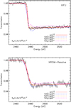 |
Fig. 4 Simulation of the sulfur K edge, using the XIFU calorimeter with an exposure time of 200 ks (top) and XRISM-Resolve with a 400 ks exposure time (bottom) of a the bright XRB GX 5–1 (F2−10 keV ~ 2.5 × 10⁻⁸ erg cm−2 s−1). The simulation considers different sulfur species with a dust depletion of 30%. |
5.2 Aluminum and calcium
The XIFU simulation shows that dust will be easily detectable, even if the edge itself produced a jump in the spectrum of only few %. However, from the Al edge alone, it would be difficult to distinguish among different compounds.
We alsonote that contrary to other extinction profiles, the scattering peak, which appears as an emission-like feature before the edge jump, is noticeable in Al. This peak is sensitive to the dust size distribution (Zeegers et al. 2017)and can be used, in principle, to estimate the mean grain size along the line of sight, for example. As described above, we also tested the effect of the dust size distribution of Draine & Fraisse (2009) for Al2 O3. The edge energy of Al lies in a zone sensitive to scattering (Draine 2003), therefore in Fig. 3 the large particles contributionis evident. As shown in Rogantini et al. (2018), the role of a substantial scattering contribution to the extinction not only forces the edge energy to shift, but may also modify the appearance of the edge absorption features. Grains containing seeds of Al and Ca, which are shielded from erosion in the ISM, are believed to be of large size because of several layers of coatings surrounding those seeds elements (e.g., Clayton 1978, and Sect. 2). With future instruments we will therefore also be able to test the presence of larger particles for less abundant, but important, constituentsof the ISM. The study of the Al edge will be however challenging, as Al is always a major component of X-ray space instruments (often in the form of foils). The extinction feature from Al in the ISM will be always blended with a relatively deep instrumental Al feature. This would need a careful calibration, adding uncertainty to the modeling.
Calciumis totally depleted in the ISM, therefore the main dust features will be detected (Fig. 5). However, calcium is mostly contained in silicates and aluminates, where oxygen is the main constituent. The XAFS models show that the first and main absorption feature is due to the nearest neighboring atom that the photoelectron wave will encounter (Lee & Ravel 2005). In the case simulated in this work, the absorption profile is dominated by oxygen (as is the case, to a lesser extend, in the Al edge), and only at higher energies are the secondary absorption features to be seen. For this reason the Ca inclusion in a specific silicate may be hard to disentangle through the observed spectrum. However, calcite (CaCO3, dashed orange line), due to its different internal structure, will show a distinctive pattern, which may be in principle disentangled. This will help determine whether this elusive compound (e.g., Kemper et al. 2002, and Sect. 2) may be present in the ISM. We tested the contribution of possible large grains on anorthite (blue dash-dotted line in Fig. 5). The contributionof larger grains does not produce a well detectable feature.
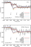 |
Fig. 5 Simulation of the calcium K edge, using the XIFU calorimeter with exposure time 400 ks, (top) and the XRISM-Resolve with a 500 ks exposure time (bottom). We used the bright XRB GX 340+00 (F2−10 keV ~ 1.3 × 10⁻⁸ erg cm−2 s−1). The simulation considers different calcium species with a dust depletion of 100%. The data have been binned for clarity. |
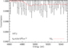 |
Fig. 6 Simulation in 500 ks of the titanium K edge, using the XIFU calorimeter, using the bright XRB GX340+00 (F2−10 keV ~ 1.3 × 10⁻⁸ erg cm−2 s−1) as template.The dust depletion is 100%. The data have been binned for clarity. |
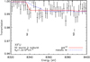 |
Fig. 7 Simulation in 300 ks of the nickel K edge, using the XIFU calorimeter, assuming that a highly absorbed source near the GC reaches in outburst the same flux level as GX340+00 (F2−10 keV ~ 1.3 × 10⁻⁸ erg cm−2 s−1). The dust depletion is 100%. The data have been binned for clarity. |
5.3 Sulfur
In the diffuse ISM, sulfur is expected to have a modest depletion (Sect. 2). We use sulfur in conjunction with iron in the form of troilite, pyrrohtite, and pyrite. FeS is a likely candidate for a diffuse interstellar environment because of its inclusion in GEMS (Bradley 1994; Bradley et al. 1999). The line of sight toward GX 5-1, at distance of ~9 kpc is also likely to cross molecular clouds and this would apply for any source located near the GC. The dust inclusion of sulfur in molecular clouds is still an open issue (Sect. 2). Some of the S must be associated with ices and carbon-hydrogen aggregates, while the rest may be in the form of FeS or atomic gas. Even the sum of all known S-bearing molecules would be unlikely to exceed few percent of the total S abundance. Therefore any significant depletion detected by XRISM or XIFU would naturally point to the role of S in GEMS. We note that this amount of S depletion would still not procure visible deviations from the observed total dust spectral energy distribution (Köhler et al. 2014).
5.4 Titanium and nickel
Owing to its extremely low abundance in the Universe, titanium will be challenging to detect (Fig. 6). Nickel is about 20 times more abundant than Ti, however Ni will be also difficult to study (Fig. 7). The large column densities required to produce a Ni edge, will also cause strong absorption by iron, whose K absorption edge lies at 7100 eV, only 1.2 keV away from that of nickel. Under the conditions of this simulation, the optical depth of iron will be around 18 times larger than that of nickel. The net effect is that the Ni edge “sees” a continuum that is much lower than that of the source, reducing the signal-to-noise ratio in that feature. Both titanium and nickel are however completely depleted in most ISM environments, therefore even a column density estimate will be useful to constrain the abundance of these two elements, which are a product of explosions of both massive stars and white dwarfs.
6 Conclusions
In this paper we have shown how improved instrumental sensitivity and resolution will help in the understanding of new aspects of the composition of ID. Our results can be summarized as follows:
Future instruments with characteristics similar to the Arcus mission will be able to disentangle between the major components of carbon, namely amorphous carbon (or graphite) and hydrogenated carbon. The effect of minor constituents of C in the ISM (e.g., nano-diamonds and PAH) will be challenging to detect.
Instruments with improved capabilities at higher energies as Athena-XIFU or XRISM-Resolve, will be able to study absorption features that, owing to their modest opacity, could not be investigated before. Simulations show that even a 1–6% jump in the transmission spectrum will be detected, allowing at least abundances measurements. For the low-cosmic abundance elements investigate in the E > 1 keV band (namely Al, S and Ca), a full characterization (e.g., distinguishing among various silicate-like compounds) of the dust chemistry will likely be challenging. However, some main distinctions can be made:
-
it will be possible to distinguish between calcium in carbonates and silicates around the Ca edge;
-
for bothCa and Al the dust size distribution of these heavily depleted elements can be determined with different precision depending on the instrument characteristics;
-
it will be possible to determine the depletion of sulfur in the ISM. This in turn will help to clarify the S inclusion in GEMS, which are sometimes considered as one of the main forms of silicates in the ISM.
Finally, simulations show that Ti and Ni will be unaccessible to a detailed study even with next generation instruments considered in this work.
Acknowledgements
Dust studies at Leiden Observatory are supported also through the Spinoza Premie of the Dutch science agency, NWO. The Netherlands Institute for Space Research is supported financially by NWO. E.C. and D.R. acknowledge the support of the NWO-VIDI grant 639.042.525. We acknowledge SOLEIL for provision of synchrotron radiation facilities and we would like to thank Delphine Vantelon for assistance in using the LUCIA beamline and Harald Mutschke for procuring the Al-bearing samples. We also thank Alessandra Candian and the anonymous referee for useful comments on the manuscript. This research made use of the Chandra Transmission Grating Catalog and archive (http://tgcat.mit.edu).
Appendix A Extinction profiles
We show here the extinction profiles in transmission, normalized for the continuum, of the compounds presented in this paper. Their formulas and literature reference are reported in Table 2. The instruments used for those measurements are reported in Table A.1.
 |
Fig. A.1 Extinction profiles of the C, Al, and S compounds presented in this paper. The dust column densities of the elements arethe same used for the simulations. The edge energy and the original energy resolution are as reported in the literature. |
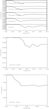 |
Fig. A.2 Extinction profiles of the Ca, Ti, and Ni compounds presented in this paper. The dust column densities of the elements are the same used for the simulations. The edge energy and the energy resolution are as reported in the literature. |
Facilities and resolution of the literature laboratory measurements.
References
- Albella, J. M., Banks, J. C., Climent-Font, A., et al. 1998, University of North Texas Libraries, digital.library.unt.edu/ark:/67531/metadc668006/ [Google Scholar]
- Barret, D., Lam Trong, T., den Herder, J.-W., et al. 2016, Proc. SPIE, 9905, 99052F [CrossRef] [Google Scholar]
- Bilalbegović, G., & Baranović, G. 2015, MNRAS, 446, 3118 [NASA ADS] [CrossRef] [Google Scholar]
- Bilalbegović, G., Maksimović, A., & Valencic, L. A. 2018, MNRAS, 476, 5358 [Google Scholar]
- Bohren, C. F. 2010, Eu. J. Phys., 31, 573 [CrossRef] [Google Scholar]
- Bonnin-Mosbah, M., Métrich, N., Susini, J., et al. 2002, Spectrochim. Acta, 57, 711 [NASA ADS] [CrossRef] [Google Scholar]
- Bradley, J. P. 1994, Science, 265, 925 [Google Scholar]
- Bradley, J. P., Keller, L. P., Snow, T. P., et al. 1999, Science, 285, 1716 [NASA ADS] [CrossRef] [PubMed] [Google Scholar]
- Buijnsters, J. G., Gago, R., Jiménez, I., et al. 2009, J. Appl. Phys., 105, 093510-093510-7 [NASA ADS] [CrossRef] [Google Scholar]
- Clayton, D. D. 1978, Moon Planets, 19, 109 [NASA ADS] [CrossRef] [Google Scholar]
- Compiègne, M., Verstraete, L., Jones, A., et al. 2011, A&A, 525, A103 [NASA ADS] [CrossRef] [EDP Sciences] [Google Scholar]
- Costantini, E., Pinto, C., Kaastra, J. S., et al. 2012, A&A, 539, A32 [NASA ADS] [CrossRef] [EDP Sciences] [Google Scholar]
- Corrales, L. R., García, J., Wilms, J., & Baganoff, F. 2016, MNRAS, 458, 1345 [NASA ADS] [CrossRef] [Google Scholar]
- Crinklaw, G., Federman, S. R., & Joseph, C. L. 1994, ApJ, 424, 748 [NASA ADS] [CrossRef] [Google Scholar]
- Decourchelle, A., Costantini, E., Badenes, C., et al. 2013, ArXiv e-prints [arXiv:1306.2335] [Google Scholar]
- Delgado-Inglada, G., Mesa-Delgado, A., García-Rojas, J., Rodríguez, M., & Esteban, C. 2016, MNRAS, 456, 3855 [NASA ADS] [CrossRef] [Google Scholar]
- Draine, B. 1989, Interstellar Dust (Dordrecht: Kluwer Academic Publishers), 135, 313 [NASA ADS] [CrossRef] [Google Scholar]
- Draine, B. T. 2003, ARA&A, 41, 241 [NASA ADS] [CrossRef] [Google Scholar]
- Draine, B. T., & Fraisse, A. A. 2009, ApJ, 696, 1 [NASA ADS] [CrossRef] [Google Scholar]
- Duley, W. W., Millar, T. J., & Williams, A. D. 1980, MNRAS, 192, 945 [NASA ADS] [Google Scholar]
- Duley, W. W., Jones, A. P., & Williams, D. A. 1989, MNRAS, 236, 709 [NASA ADS] [Google Scholar]
- Edgar, R. J., & Savage, B. D. 1989, ApJ, 340, 762 [NASA ADS] [CrossRef] [Google Scholar]
- Federman, S. R., Sheffer, Y., Lambert, D. L., & Gilliland, R. L. 1993, ApJ, 413, L51 [NASA ADS] [CrossRef] [Google Scholar]
- Ferrarotti, A. S., & Gail, H.-P. 2005, A&A, 430, 959 [NASA ADS] [CrossRef] [EDP Sciences] [Google Scholar]
- Ferrarotti, A. S., & Gail, H.-P. 2006, A&A, 447, 553 [NASA ADS] [CrossRef] [EDP Sciences] [Google Scholar]
- Field, G. B. 1974, ApJ, 187, 453 [NASA ADS] [CrossRef] [Google Scholar]
- Fitzpatrick, E. L., & Massa, D. 2007, ApJ, 663, 320 [NASA ADS] [CrossRef] [EDP Sciences] [Google Scholar]
- Gainsforth, Z., Butterworth, A., Fakra, S., et al. 2007, Lunar Planet. Sci. Conf., 38, 2273 [NASA ADS] [Google Scholar]
- Gorczyca, T. W., Bautista, M. A., Hasoglu, M. F., et al. 2013, ApJ, 779, 78 [NASA ADS] [CrossRef] [Google Scholar]
- Gry, C., & Jenkins, E. B. 2017, A&A, 598, A31 [NASA ADS] [CrossRef] [EDP Sciences] [Google Scholar]
- Henke, B. L., Gullikson, E. M., & Davis, J. C. 1993, At. Data Nucl. Data Tables, 54, 181 [NASA ADS] [CrossRef] [Google Scholar]
- Hoffman, J., & Draine, B. T. 2016, ApJ, 817, 139 [NASA ADS] [CrossRef] [Google Scholar]
- Hony, S., Waters, L. B. F. M., & Tielens, A. G. G. M. 2002, A&A, 390, 533 [NASA ADS] [CrossRef] [EDP Sciences] [Google Scholar]
- Hunter, I., Smoker, J. V., Keenan, F. P., et al. 2006, MNRAS, 367, 1478 [CrossRef] [Google Scholar]
- Jansen, F., Lumb, D., Altieri, B., et al. 2001, A&A, 365, L1 [NASA ADS] [CrossRef] [EDP Sciences] [Google Scholar]
- Jenkins, E. B. 2009, ApJ, 700, 1299 [NASA ADS] [CrossRef] [Google Scholar]
- Jenkins, E. B., & Wallerstein, G. 1996, ApJ, 462, 758 [NASA ADS] [CrossRef] [Google Scholar]
- Jiménez-Escobar, A., & Muñoz Caro, G. M. 2011, A&A, 536, A91 [NASA ADS] [CrossRef] [EDP Sciences] [Google Scholar]
- Jones, A. P., Köhler, M., Ysard, N., Bocchio, M., & Verstraete, L. 2017, A&A, 602, A46 [NASA ADS] [CrossRef] [EDP Sciences] [Google Scholar]
- Joseph, C. L., Snow, T. P., Jr., Seab, C. G., & Crutcher, R. M. 1986, ApJ, 309, 771 [NASA ADS] [CrossRef] [Google Scholar]
- Juett, A. M., Schulz, N. S., & Chakrabarty, D. 2004, ApJ, 612, 308 [NASA ADS] [CrossRef] [Google Scholar]
- Kaastra, J. S., Mewe, R., & Nieuwenhuijzen, H. 1996, UV and X-ray Spectroscopy of Astrophysical and Laboratory Plasmas, 411 [Google Scholar]
- Keller, L. P., & Messenger, S. 2008, Lunar Planet. Sci. Conf., 39, 2347 [NASA ADS] [Google Scholar]
- Keller, L. P., Hony, S., Bradley, J. P., et al. 2002, Nature, 417, 148 [NASA ADS] [CrossRef] [PubMed] [Google Scholar]
- Keller, L. P., Loeffler, M. J., Christoffersen, R., et al. 2010, Lunar Planet. Sci. Conf., 41, 1172 [NASA ADS] [Google Scholar]
- Kemper, F., Jäger, C., Waters, L. B. F. M., et al. 2002, Nature, 415, 295 [NASA ADS] [CrossRef] [PubMed] [Google Scholar]
- Köhler, M., Jones, A., & Ysard, N. 2014, A&A, 565, L9 [NASA ADS] [CrossRef] [EDP Sciences] [Google Scholar]
- Lee, J. C., & Ravel, B. 2005, ApJ, 622, 970 [NASA ADS] [CrossRef] [Google Scholar]
- Lee, J. C., Reynolds, C. S., Remillard, R., et al. 2002, ApJ, 567, 1102 [NASA ADS] [CrossRef] [Google Scholar]
- Lee, J. C., Xiang, J., Ravel, B., Kortright, J., & Flanagan, K. 2009, ApJ, 702, 970 [NASA ADS] [CrossRef] [Google Scholar]
- Lewis, R. S., Ming, T., Wacker, J. F., Anders, E., & Steel, E. 1987, Nature, 326, 160 [NASA ADS] [CrossRef] [Google Scholar]
- Lodders, K. 2010, Astrophys. Space Sci. Proc., 16, 379 [NASA ADS] [CrossRef] [Google Scholar]
- Mathis, J. S., Rumpl, W., & Nordsieck, K. H. 1977, ApJ, 217, 425 [NASA ADS] [CrossRef] [Google Scholar]
- McMaster, W. H., Kerr Del Grande, N., Mallett, J. H., & Hubbell, J. H. 1970, At. Data Nucl. Data Tables, 8, 443 [NASA ADS] [CrossRef] [Google Scholar]
- Mie, G. 1908, Ann. Phys., 330, 377 [Google Scholar]
- Mitsuda, K., Kelley, R. L., Akamatsu, H., et al. 2014, Proc. SPIE, 9144, 91442A [Google Scholar]
- Nandra, K., Barret, D., Barcons, X., et al. 2013, ArXiv e-prints [arXiv:1306.2307] [Google Scholar]
- Neuville, D. R., Cormier, L., Roux, J., et al. 2007, X-ray Absorption Fine Structure - XAFS13, 882, 413 [NASA ADS] [CrossRef] [Google Scholar]
- Paerels, F., Brinkman, A. C., van der Meer, R. L. J., et al. 2001, ApJ, 546, 338 [NASA ADS] [CrossRef] [Google Scholar]
- Pinto, C., Kaastra, J. S., Costantini, E., & Verbunt, F. 2010, A&A, 521, A79 [NASA ADS] [CrossRef] [EDP Sciences] [Google Scholar]
- Pinto, C., Kaastra, J. S., Costantini, E., & de Vries, C. 2013, A&A, 551, A25 [NASA ADS] [CrossRef] [EDP Sciences] [Google Scholar]
- Rehr, J. J., & Albers, R. C. 2000, Rev. Mod. Phys., 72, 621 [NASA ADS] [CrossRef] [Google Scholar]
- Reitsma, G., Boschman, L., Deuzeman, M. J., et al. 2014, Phys. Rev. Lett., 113, 053002 [NASA ADS] [CrossRef] [PubMed] [Google Scholar]
- Reitsma, G., Boschman, L., Deuzeman, M. J., et al. 2015, J. Chem. Phys., 142, 024308 [NASA ADS] [CrossRef] [Google Scholar]
- Rogantini, D., Costantini, E., Zeegers, S. T., et al. 2018, A&A, 609, A22 [NASA ADS] [CrossRef] [EDP Sciences] [Google Scholar]
- Schattenburg, M. L., & Canizares, C. R. 1986, ApJ, 301, 759 [NASA ADS] [CrossRef] [Google Scholar]
- Schneider, P. C., & Schmitt, J. H. M. M. 2010, A&A, 516, A8 [NASA ADS] [CrossRef] [EDP Sciences] [Google Scholar]
- Schulz, N. S., Corrales, L., & Canizares, C. R. 2016, ApJ, 827, 49 [NASA ADS] [CrossRef] [Google Scholar]
- Sembach, K. R., & Savage, B. D. 1996, ApJ, 457, 211 [NASA ADS] [CrossRef] [Google Scholar]
- Shin, S. I., Go, A., Kim, I. Y., et al. 2013, Energy Environ. Sci., 6, 608 [CrossRef] [Google Scholar]
- Siebenmorgen, R., & Krügel, E. 2010, A&A, 511, A6 [NASA ADS] [CrossRef] [EDP Sciences] [Google Scholar]
- Smith, R. K., Abraham, M. H., Allured, R., et al. 2016, Proc. SPIE, 9905, 99054M [NASA ADS] [CrossRef] [Google Scholar]
- Snow, T. P., Jr. 1975, ApJ, 202, L87 [NASA ADS] [CrossRef] [Google Scholar]
- Snow, T. P., Destree, J. D., & Jensen, A. G. 2007, ApJ, 655, 285 [NASA ADS] [CrossRef] [Google Scholar]
- Sofia, U. J., & Jenkins, E. B. 1998, ApJ, 499, 951 [NASA ADS] [CrossRef] [Google Scholar]
- Stern, E. A., Newville, M., Ravel, B., Yacoby, Y., & Haskel, D. 1995, Phys. B Condens. Matter, 208, 117 [Google Scholar]
- Tielens, A. G. G. M. 2001, Tetons 4: Galactic Structure, Stars and the Interstellar Medium (San Francisco: ASP), 231, 92 [NASA ADS] [Google Scholar]
- Tielens, A. G. G. M. 2013, Rev. Mod. Phys., 85, 1021 [NASA ADS] [CrossRef] [Google Scholar]
- Tielens, A. G. G. M., Seab, C. G., Hollenbach, D. J., & McKee, C. F. 1987, ApJ, 319, L109 [NASA ADS] [CrossRef] [Google Scholar]
- Trivedi, B. M. P., & Larimer, J. W. 1981, ApJ, 248, 563 [NASA ADS] [CrossRef] [Google Scholar]
- Turner, B. E. 1991, ApJ, 376, 573 [NASA ADS] [CrossRef] [Google Scholar]
- Ueda, Y., Mitsuda, K., Murakami, H., et al. 2005, ApJ, 620, 274 [NASA ADS] [CrossRef] [Google Scholar]
- Valencic, L. A., & Smith, R. K. 2013, ApJ, 770, 22 [NASA ADS] [CrossRef] [Google Scholar]
- van de Hulst, H. C. 1957, Light Scattering by Small Particles (New York: John Wiley & Sons, Inc.) [Google Scholar]
- Van Kerckhoven, C., Tielens, A. G. G. M., & Waelkens, C. 2002, A&A, 384, 568 [NASA ADS] [CrossRef] [EDP Sciences] [Google Scholar]
- Van Loon, L. L., Throssell, C., & Dutton, M. D. 2015, Environ. Sci. Processes Impacts, 2015, 922 [CrossRef] [Google Scholar]
- Verner, D. A., Ferland, G. J., Korista, K. T., & Yakovlev, D. G. 1996, ApJ, 465, 487 [NASA ADS] [CrossRef] [Google Scholar]
- Vidal, T. H. G., Loison, J.-C., Jaziri, A. Y., et al. 2017, MNRAS, 469, 435 [NASA ADS] [CrossRef] [Google Scholar]
- Voit, G. M. 1992, MNRAS, 258, 841 [NASA ADS] [CrossRef] [Google Scholar]
- Wakelam, V., & Herbst, E. 2008, ApJ, 680, 371 [NASA ADS] [CrossRef] [Google Scholar]
- Wasson, J. T. 1985, Meteorites: Their Record of Early Solar-System History (New York: W. H. Freeman and Co.), 1985, 274 [NASA ADS] [Google Scholar]
- Weisskopf, M. C. 1999, ArXiv e-prints [arXiv:astro-ph/9912097] [Google Scholar]
- Welty, D. E., & Crowther, P. A. 2010, MNRAS, 404, 1321 [NASA ADS] [Google Scholar]
- Westphal, A. J., Stroud, R. M., Bechtel, H. A., et al. 2014, Science, 345, 786 [NASA ADS] [CrossRef] [Google Scholar]
- Whittet, D. C. B. 2003, Dust in the Galactic Environment, Series in Astronomy and Astrophysics, 2nd edn., ed. D.C.B. Whittet (Bristol: Institute of Physics Publishing) [Google Scholar]
- Whittet, D. C. B. 2011, Astronomical Polarimetry 2008: Science from Small to Large Telescopes, 93 [Google Scholar]
- Wiscombe, W. J. 1980, Appl. Opt., 19, 1505 [NASA ADS] [CrossRef] [PubMed] [Google Scholar]
- Wooden, D. H. 2008, Space Sci. Rev., 138, 75 [NASA ADS] [CrossRef] [Google Scholar]
- Zeegers, S. T., Costantini, E., de Vries, C. P., et al. 2017, A&A, 599, A117 [NASA ADS] [CrossRef] [EDP Sciences] [Google Scholar]
- Zeegers, S. T., Costantini, E., Rogantini, D., et al. 2019, A&A, 627, A16 [NASA ADS] [CrossRef] [EDP Sciences] [Google Scholar]
All Tables
Parameters of the instruments used in the simulations at the energy of the elements studied in this work.
All Figures
|
Fig. 1 Top panel: abundance pattern as a function of energy for the absorbing elements in the X-ray band. The K-edge energy is indicated, except from Fe, for which both the K and the L edges, at 7.1 and ~0.7 keV, respectively, can be studied. Abundances follow Lodders (2010) and they are expressed in terms of log (X/H)+12. In this frame, the abundance of hydrogen is 12. The open diamonds indicate the elements that are accessible by current instruments. The triangles indicate the relevant elements that will be accessible by future instruments to study dust. The black triangles indicate the subject of this work. Middle panel: range of depletions as reported by Jenkins (2009) for all elements, except C (Jenkins 2009; Whittet 2003), F (Snow et al. 2007), Na (Turner 1991), S (Gry & Jenkins 2017), K (Snow 1975), Ca (Crinklaw et al. 1994), Co (Federman et al. 1993), Al (Jenkins & Wallerstein 1996), and Ar (Sofia & Jenkins 1998). Bottom panel: energy range covered by present and future (red)mission. The solid line highlights the energy range for which the instruments capabilities are optimal for observing absorption by dust. |
| In the text | |
|
Fig. 2 Simulation in 500 ks of carbon K edge, using the Arcus grating, of an XRB in high state (F0.5−2 keV ~ 3 × 10⁻⁹ erg cm−2 s−1). The simulation considers different carbon species with a dust depletion of 60%. The two absorption lines belong to the atomic phase of C, namely C I. |
| In the text | |
|
Fig. 3 Simulation in 300 ks of the aluminum K edge, using the XIFU calorimeter, of the bright XRB GX 3+1 (F2−10 keV ~ 3 × 10⁻⁹ erg cm−2 s−1). The dust depletion is 100%. The data have been binned for clarity. |
| In the text | |
|
Fig. 4 Simulation of the sulfur K edge, using the XIFU calorimeter with an exposure time of 200 ks (top) and XRISM-Resolve with a 400 ks exposure time (bottom) of a the bright XRB GX 5–1 (F2−10 keV ~ 2.5 × 10⁻⁸ erg cm−2 s−1). The simulation considers different sulfur species with a dust depletion of 30%. |
| In the text | |
|
Fig. 5 Simulation of the calcium K edge, using the XIFU calorimeter with exposure time 400 ks, (top) and the XRISM-Resolve with a 500 ks exposure time (bottom). We used the bright XRB GX 340+00 (F2−10 keV ~ 1.3 × 10⁻⁸ erg cm−2 s−1). The simulation considers different calcium species with a dust depletion of 100%. The data have been binned for clarity. |
| In the text | |
|
Fig. 6 Simulation in 500 ks of the titanium K edge, using the XIFU calorimeter, using the bright XRB GX340+00 (F2−10 keV ~ 1.3 × 10⁻⁸ erg cm−2 s−1) as template.The dust depletion is 100%. The data have been binned for clarity. |
| In the text | |
|
Fig. 7 Simulation in 300 ks of the nickel K edge, using the XIFU calorimeter, assuming that a highly absorbed source near the GC reaches in outburst the same flux level as GX340+00 (F2−10 keV ~ 1.3 × 10⁻⁸ erg cm−2 s−1). The dust depletion is 100%. The data have been binned for clarity. |
| In the text | |
|
Fig. A.1 Extinction profiles of the C, Al, and S compounds presented in this paper. The dust column densities of the elements arethe same used for the simulations. The edge energy and the original energy resolution are as reported in the literature. |
| In the text | |
|
Fig. A.2 Extinction profiles of the Ca, Ti, and Ni compounds presented in this paper. The dust column densities of the elements are the same used for the simulations. The edge energy and the energy resolution are as reported in the literature. |
| In the text | |
Current usage metrics show cumulative count of Article Views (full-text article views including HTML views, PDF and ePub downloads, according to the available data) and Abstracts Views on Vision4Press platform.
Data correspond to usage on the plateform after 2015. The current usage metrics is available 48-96 hours after online publication and is updated daily on week days.
Initial download of the metrics may take a while.