© L. Blanchet et al. 2019

1. Introduction

Whereas more than 4000 exoplanets have been discovered so far, the planet orbiting the G5 star HD 80606 remains a remarkable and unique case. Its eccentricity is extremely high: e ≃ 0.93. HD 20782b is the only planet reported to have a higher eccentricity (O’Toole et al. 2009) but its high e-value stands on one single measurement and has not been confirmed up to now. The high eccentricity of HD 80606b was well established as soon as the planet was discovered through radial velocity measurements (Naef et al. 2001) and has been largely confirmed by subsequent observations. Today the most accurate system parameters are those determined by Hébrard et al. (2011), who provide e = 0.9330 ± 0.0005.

The long orbital period of the planet (P  =  111.4367 ± 0.0004 days) implied a low probability of the orbital plan to be aligned with the line of sight to the Earth. Still, HD 80606b was successively discovered to pass behind its parent star (planetary eclipses) by Laughlin et al. (2009), then in front of it (planetary transits) by Moutou et al. (2009; see also Garcia-Melendo & McCullough 2009; Fossey et al. 2009; Winn et al. 2009; Hidas et al. 2010). That configuration allows the planetary radius to be measured (R_p  =  0.981 ± 0.023 R_Jup); the inclination of the orbit is also known (i = 89.269 ° ±0.018°), which provides the mass M_p = 4.08 ± 0.14 M_Jup from the sky-projected mass derived with radial velocities. The obliquity of the system could also be measured from the Rossiter–McLaughlin anomaly observed during transits, which revealed that the orbit of HD 80606b is prograde but inclined (Moutou et al. 2009; Pont et al. 2009; Winn et al. 2009); Hébrard et al. (2011) reported an obliquity of λ = 42 ° ±8°. Such a peculiar orbit may be explained by the influence of the companion star HD 80607, located 1200 AU further away, through a Kozai–Lidov mechanism (Pont et al. 2009; Correia et al. 2011).

The particularly high eccentricity of the planetary orbit raises the question of the feasibility of detecting the general relativistic (GR) precession of its periastron. Indeed it should be enhanced to

$$\begin{array}{c}\hfill {\mathrm{\Delta }}_{\mathrm{GR}}=\frac{6\pi GM}{a{c}^2(1-e^2)}\simeq 215\mathrm{arcsec}/\mathrm{century},\end{array}$$(1)

as compared to 43 arcsec/century for Mercury (see also Correia et al. 2011).

Besides Mercury, the relativistic precession has been measured in the solar system for some asteroids like Icarus (Gilvarry 1953). The tests done in the solar system agree with GR to within 10⁻⁴ (Will 1993). Outside the solar system the effect is well known in binary pulsars like the Hulse–Taylor pulsar (Hulse & Taylor 1975) where it has been measured with high precision (see Taylor & Weisberg 1982), and in other binary pulsars such as the double pulsar (Kramer et al. 2006). To a further distance, there are now attempts to measure the relativistic precession of the star S2 close to the galactic centre (Parsa et al. 2017). The measure of the relativistic periastron advance in stellar systems was proposed by Gimenez (1985), but it is quite complicated to discriminate it from the tidal precession (see e.g. Wolf et al. 2010).

Figueira et al. (2016) reported that the relativistic precession was not detectable in the HD 80606 system in spite of the large dataset secured over several years. They measured the variation of the longitude of the periastron using the whole available datasets: $\dot{\omega }=9720\pm 11160\text{arcsec}/\text{century}$, thus in a non-significant way. Indeed, the accuracy reached on ω mainly from radial velocities is ±540 arcsec (Hébrard et al. 2011), which is not accurate enough.

The transiting nature of HD 80606b allows a better accuracy to be reached thanks to the precise timing that can be measured on the mid-point of each transit or eclipse. Typical accuracies of ±85 s (Hébrard et al. 2011) and ±260 s (Laughlin et al. 2009) were obtained on the mid-point of transits and eclipses, respectively, using the Spitzer Space Telescope and its IRAC instruments. Indeed, only a satellite on an Earth-trailing heliocentric orbit such as Spitzer could allow the whole 12-hour-long transit of HD 80606b to be continuously observed together with sufficiently long off-transit references immediately before and after the event.

In this paper we propose to detect the GR precession of the periastron (and the relativistic orbital motion) for the exoplanet HD 80606b by using a method based on the transit times, computing a small drift in the successive instants of transits due to relativity. We find that in ten years (after 33 periods), due to the relativistic effects, the instants of transits are delayed with respect to the Newtonian predicted ones by about three minutes. Whereas the transit mid-time could be measured with such an accuracy, the absolute value of that shift could not be detected because the system’s orbital parameters are not known today with a high enough accuracy.

However, we argue that the effect could actually be measurable from the observation of the change of the elapsed time t_{tr − ec} = t_tr − t_ec between an eclipse and the next transit¹. The time between an eclipse and a transit was measured in January 2010 using Spitzer to be

$$\begin{array}{c}\hfill t_{\mathrm{tr}-\mathrm{ec}}(\text{Jan.}2010)\simeq 5.9\text{days},\end{array}$$(2)

with a good accuracy of ±275 s. Due to the GR precession of the periastron, and the modification of the period due to relativity, we find that this time difference will be reduced by 183 s in 2020 (after 33 orbits), and by 271 s in 2024 (49 orbits). Such shift would be difficult to detect in 2020 using IRAC on Spitzer, but should be detectable a few years later using NIRCam or MIRI on James Webb Space Telescope (JWST).

Most of the paper is devoted to theoretical aspects, and it ends with a conclusion and discussion in Sect. 6 where we give further comments on previous observations and on the Newtonian perturbing effects. In Sect. 2 we introduce the geometrical conventions used to compute the times of transits and eclipses. Those are computed in two different ways: a post-Keplerian parametrisation of the orbit in Sect. 3, and a Hamiltonian method using Delaunay-Poincaré canonical variables in Sect. 4. Those methods give the exact solution of the first post-Newtonian equations of motion. Our final results for the transit times are given in Tables 1–3 below. Furthermore, as a check of the latter methods, we also computed the transit times with a method relying on celestial-mechanics perturbation theory in Sect. 5. As we used it, this procedure is valid on average over one orbit, and takes only into account the secular effects. We find that it is in good agreement with the post-Keplerian and the Hamiltonian methods. A quick but rough estimate of the GR shift of transit times is also given in Appendix A.

2. Geometry of the planetary transits

We introduce a frame {x, y, z} with origin at the centre of the star. The observer is in the direction x (Earth’s direction), while the projected angular momentum of the star is by convention along the direction z. Hence the plane {y, z} is the plane of the sky. The orbital plane of the planet is defined by its inclination I with respect to the plane {x, y}, and by its longitude Ω with respect to the plane {x, z}, following our conventions described in Fig. 1a. As depicted in Fig. 1c, the motion of the planet in the orbital plane is parametrised by polar coordinates (r, φ), where φ denotes the sum of the true anomaly and of ω₀, the latter denoting a constant angle, which can be viewed as defining the initial argument of the periastron at a reference time. Then the coordinates (x, y, z) of the planet in this frame read (see Figs. 1a and c)

$$\begin{array}{cc}\hfill x& =r[-cos\phi cos\mathrm{\Omega }+sin\phi cosIsin\mathrm{\Omega }],\hfill \end{array}$$(3a)

$$\begin{array}{cc}\hfill y& =r[-cos\phi sin\mathrm{\Omega }-sin\phi cosIcos\mathrm{\Omega }],\hfill \end{array}$$(3b)

$$\begin{array}{cc}\hfill z& =rsin\phi sinI.\hfill \end{array}$$(3c)

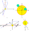Fig. 1. Geometry of the planetary transit: (a) Motion of the planet with respect to the observer, located at infinity in the direction of x of the frame {x, y, z}. The centre of the star is denoted O, P is the periastron at reference time tP, and J⋆ is the angular momentum of the star projected on the plane of the sky {y, z}. (b) The transit as seen by the observer and the definition of the points {Ti}; here are only shown T1 and T3. (c) The trajectory of the planet and the points {Ti} (transit) and $\{{\overline{T}}_i\}$ (eclipse) as seen in the orbital plane {X, Y}. Up to an angle Ω, the observer is in the direction of X. (d) View of the transit from above. The direction (ON) is the line of “nodes”, corresponding to (OX) in (a).

Since x is the direction of the observer, the condition for the (partial or complete) transit of the planet is that y² + z² ≤ (R_⋆ + R_p)², where R_⋆ and R_p are the radius of the star and planet, hence

$$\begin{array}{c}\hfill {sin}^{2}I{sin}^2\phi +(cosIcos\mathrm{\Omega }sin\phi +sin\mathrm{\Omega }cos\phi {)}^2⩽{\left(\frac{R_{\star }+R_{\mathrm{p}}}{r}\right)}^2.\end{array}$$(4)

Since R_⋆ + R_p ≪ r, it is easy to see that this condition can be satisfied when sin I ≪ 1 or sin φ ≪ 1, and |cos I cos Ωsinφ + sinΩcosφ|≪1. With the conventions of Fig. 1a we are interested in a transit for which φ ≃ π and Ω ≃ 0². On the other hand, for an eclipse during which the planet is passing beyond the star as seen from the observer, we have φ ≃ 0 and Ω ≃ 0. In an expansion to the first order in $\frac{R_{\star }+R_{\mathrm{p}}}{r}\ll 1,$ we find that the coordinates of the planet during and around the transit are

$$\begin{array}{cc}\hfill x& \simeq \frac{b}{sinI}[cot\mathrm{\Omega }+cosIsin\phi ],\hfill \end{array}$$(5a)

$$\begin{array}{cc}\hfill y& \simeq \frac{b}{sinI}[1-\frac{sin\phi cosI}{sin\mathrm{\Omega }}],\hfill \end{array}$$(5b)

$$\begin{array}{cc}\hfill z& \simeq \frac{bsin\phi }{sin\mathrm{\Omega }},\hfill \end{array}$$(5c)

where the impact parameter b of the planet is the distance between the trajectory of the planet projected on the plane {y, z} and the centre of the star. Neglecting the bending of the trajectory during the transit and eclipses³, the impact parameter is given by (see Fig. 1b)

$$\begin{array}{c}\hfill b=\{\begin{array}{c}r(\pi )sin\mathrm{\Omega }sinI(\text{transits}{T}_i),\hfill \\ r(0)sin\mathrm{\Omega }sinI(\text{eclipses}{\overline{T}}_i),\hfill \end{array}\end{array}$$(6)

where r(π) and r(0) are the values of the radial coordinate of the planet at φ = π and φ = 0, when the transit and eclipse occur. Since the eclipse will be seen from behind the star and so much farther away, we shall have to add to the instants of eclipse a Roemer time delay accounting for the propagation of light at finite velocity c, and which is a 0.5PN effect ∝1/c. Thus ${\overline{t}}_i⟶{\overline{t}}_i+\mathrm{\Delta }{t}_{}\text{R}$ where

$$\begin{array}{c}\hfill \mathrm{\Delta }{t}_{}\text{R}=\frac{r(0)+r(\pi )}{c}\simeq 2.7\min (\mathrm{for}\mathrm{HD}80606b).\end{array}$$(7)

We define the positions of the planet {T₁, T₂, T₃, T₄} to be respectively the entry of the transit, the start of the full transit, and the exits of the full and partial transits. Similarly the points $\{{\overline{T}}_1,{\overline{T}}_2,{\overline{T}}_3,{\overline{T}}_4\}$ corresponding to the eclipse are shown in Fig. 1c. The transit and eclipse conditions for the polar coordinates (r, φ) at the passage of these points read

$$\begin{array}{c}\hfill rsin\phi =Y(b).\end{array}$$(8)

Given a model r(φ) for the planetary orbit, this determines the true anomaly φ for each of these points, where the vertical coordinate Y(b) is given in terms of the impact parameter b by (see Figs. 1b and c)

$$\begin{array}{c}\hfill Y(b)=\{\begin{array}{c}\sqrt{{(R_{\star }+R_{\mathrm{p}})}^2-b^2}+bcotI(T_1\mathrm{and}{\overline{T}}_4),\hfill \\ \sqrt{{(R_{\star }-R_{\mathrm{p}})}^2-b^2}+bcotI(T_2\mathrm{and}{\overline{T}}_3),\hfill \\ -\sqrt{{(R_{\star }-R_{\mathrm{p}})}^2-b^2}+bcotI(T_3\mathrm{and}{\overline{T}}_2),\hfill \\ -\sqrt{{(R_{\star }+R_{\mathrm{p}})}^2-b^2}+bcotI(T_4\mathrm{and}{\overline{T}}_1).\hfill \end{array}\end{array}$$(9)

The cases for which (R_⋆ ± R_p)² = b² correspond to the planet just grazing tangentially the star, either from the exterior or from the interior of the stellar disc. In addition to Eqs. (8) and (9) we compute also the points corresponding to the minimal approach to the center of the star, T_m and ${\overline{T}}_{\mathrm{m}}$, whose transit conditions are obviously (see Fig. 1b)

$$\begin{array}{c}\hfill Y(b)=bcotI(T_{\mathrm{m}}\mathrm{and}{\overline{T}}_{\mathrm{m}}).\end{array}$$(10)

Having determined the polar coordinates of the planet we shall deduce the instants t_i and ${\overline{t}}_i$ of passage at each of these points by using the law of motion of the planet on the trajectory.

3. Post-Newtonian motion of the planet

In this section we compute the times of transits and eclipses, that is, the instants of the successive passages at the positions T_i and ${\overline{T}}_i$ defined by the geometric conditions in Eqs. (8)–(10), in a relativistic model, including the first post-Newtonian (1PN) corrections beyond a Keplerian orbit. More precisely, we compute the difference between the transit times predicted by the relativistic 1PN model and those predicted by the Newtonian model. This will permit us to assess whether the latter relativistic corrections could be detectable, and we propose an observable quantity, directly measurable in future observations of the planet HD 80606b.

3.1. Keplerian parametrisation of the orbit

In the Keplerian model the orbit of the planet and its motion on the orbit are given by the usual six orbital elements {a, e, I, ℓ, ω₀, Ω}, where I and Ω specify the orbital plane (see Fig. 1a), a is the semi-major axis, e is the eccentricity, ω₀ denotes the constant angular position of the periastron, and the mean anomaly ℓ is defined by ℓ = n₀(t − t_0, P), where t_0, P is the instant of passage at the periastron and n₀ = 2π/P₀ is the mean motion, with P₀ the period. The Keplerian relative orbit in polar coordinates (r, φ), is conveniently parametrised by the eccentric anomaly ψ as

$$\begin{array}{cc}\hfill r& =a(1-ecos\psi ),\hfill \end{array}$$(11a)

$$\begin{array}{cc}\hfill \ell & =\psi -esin\psi ,\hfill \end{array}$$(11b)

$$\begin{array}{cc}\hfill \phi & ={\omega }_0+2arctan(\sqrt{\frac{1+e}{1-e}}tan\frac{\psi }{2}).\hfill \end{array}$$(11c)

The relative orbit in polar coordinates reads

$$\begin{array}{c}\hfill r=\frac{a(1-e^2)}{1+ecos(\phi -{\omega }_0)},\end{array}$$(12)

from which we deduce the impact parameter in the Newtonian model, say b₀, to be

$$\begin{array}{c}\hfill b_0=\{\begin{array}{c}a(1-e^2)\frac{sin\mathrm{\Omega }sinI}{1-ecos{\omega }_0}(\text{transits}{T}_i),\hfill \\ a(1-e^2)\frac{sin\mathrm{\Omega }sinI}{1+ecos{\omega }_0}(\text{eclipses}{\overline{T}}_i).\hfill \end{array}\end{array}$$(13)

In the Newtonian model we have Kepler’s third law n₀ = (GM/a³)^1/2, where M = M_⋆ + M_p is the total mass of the star plus planet system. Furthermore the energy and the angular momentum of the orbit are given by the usual Keplerian formulas

$$\begin{array}{cc}\hfill E& =-\frac{GM\mu }{2a},\hfill \end{array}$$(14a)

$$\begin{array}{cc}\hfill J& =\mu \sqrt{GMa(1-e^2)},\hfill \end{array}$$(14b)

where μ = M_⋆M_p/M is the reduced mass.

The conditions for the transits and eclipses are given by Eqs. (8) with (9), and determine the values of the eccentric anomaly at these points. In the Newtonian analysis the eccentric anomaly ψ₀ is obtained by solving

$$\begin{array}{c}\hfill a[\sqrt{1-e^2}sin{\psi }_{0}cos{\omega }_0+(cos{\psi }_0-e)sin{\omega }_0]=Y_0,\end{array}$$(15)

where Y₀ = Y(b₀) denotes the vertical coordinate (Eq. (9)) computed with the Newtonian impact parameter given by Eq. (13).

3.2. Relativistic corrections to the Keplerian motion

Next we consider the relativistic 1PN model see (e.g. Wagoner & Will 1976). For this we shall use an explicit solution of the equations of motion that is particularly elegant, called the quasi-Keplerian representation of the 1PN motion (Damour & Deruelle 1985). In this representation the orbit and motion are parametrised by the eccentric anomaly ψ in a Keplerian-looking form as

$$\begin{array}{cc}\hfill r& =a_r(1-e_{r}cos\psi ),\hfill \end{array}$$(16a)

$$\begin{array}{cc}\hfill \ell & =\psi -e_{t}sin\psi ,\hfill \end{array}$$(16b)

$$\begin{array}{cc}\hfill \phi & ={\omega }_0+2Karctan(\sqrt{\frac{1+e_{\phi }}{1-e_{\phi }}}tan\frac{\psi }{2}),\hfill \end{array}$$(16c)

where ℓ = n(t − t_p) and n = 2π/P, with now P being the period of the relativistic model. The motion is parametrised by six constants: the mean motion n, a particular definition of semi-major axis a_r differing from a in the Newtonian model by a small 1PN term, the precession of the orbit K including the relativistic precession, and three types of eccentricities e_r, e_t, and e_φ differing from e and from each other by small 1PN terms. We shall pose

$$\begin{array}{cc}& n=n_0(1+\zeta ),K=1+k,a_r=a(1+\xi ),\hfill \end{array}$$(17a)

$$\begin{array}{cc}& e_r=e+{\epsilon }_r,e_t=e+{\epsilon }_t,e_{\phi }=e+{\epsilon }_{\phi }.\hfill \end{array}$$(17b)

The constant k denotes the relativistic advance of the periastron per orbital revolution, which is $k=\frac{\mathrm{\Delta }}{2\pi }$ where Δ is the angle of return to the periastron, and whose GR value has been given in Eq. (1). The effect of precession can be seen clearly with the expression of the relative orbit in polar coordinates, which takes the more involved form (Damour & Deruelle 1985)

$$\begin{array}{c}\hfill r=\frac{a_r(1-e_r^2)}{1+e_{r}cos[\frac{\phi -{\omega }_0}{K}-\frac{1}{6}k{e}_r\nu sin(\frac{\phi -{\omega }_0}{K})]}·\end{array}$$(18)

Besides the usual contribution of the precession $\propto \frac{\phi -{\omega }_0}{K}$, we note the presence of a term vanishing in the small mass ratio limit, when ν = μ/M → 0.

Crucial to the post-Keplerian formalism are the explicit expressions of all these constants in terms of the conserved energy E and angular momentum J of the orbit. Since we want to compare the relativistic model of Eq. (16) to the Newtonian one of Eq. (11) we will compare, for convenience, orbits that have the same energy E and angular momentum J. Thus we need to express the relations in terms of the “Newtonian” semi-major axis a and eccentricity e defined in terms of E and J by the Newtonian formulas in Eq. (14). We have (Damour & Deruelle 1985; see also Blanchet 2014)

$$\begin{array}{cc}& \zeta =\frac{\mathit{GM}}{8a{c}^2}(-15+\nu ),\hfill \end{array}$$(19a)

$$\begin{array}{cc}& k=\frac{3GM}{a{c}^2(1-e^2)},\hfill \end{array}$$(19b)

$$\begin{array}{cc}& \xi =\frac{\mathit{GM}}{4a{c}^2}(-7+\nu ),\hfill \end{array}$$(19c)

$$\begin{array}{cc}& {\epsilon }_r=\frac{\mathit{GM}}{8a{c}^2}[\frac{9+\nu }{e}+(15-5\nu )e],\hfill \end{array}$$(19d)

$$\begin{array}{cc}& {\epsilon }_t=\frac{\mathit{GM}}{8a{c}^2}[\frac{9+\nu }{e}+(-17+7\nu )e],\hfill \end{array}$$(19e)

$$\begin{array}{cc}& {\epsilon }_{\phi }=\frac{\mathit{GM}}{8a{c}^2}[\frac{9+\nu }{e}+(15-\nu )e].\hfill \end{array}$$(19f)

Among the effects described by these constants, the main ones are those associated with the mean motion n and the periastron precession K. The expressions for n and K in terms of E and J are invariant, meaning they do not depend on the coordinate system. Since

$$\begin{array}{c}\hfill \frac{k}{\zeta }=-\frac{24}{(15-\nu )(1-e^2)}\simeq -12(\mathrm{for}\mathrm{HD}80606\mathrm{b}),\end{array}$$(20)

we expect the effect of the precession of the orbit to be dominant over the shift in the orbital period. The other relations, linking the semi-major axis and eccentricities to E and J, depend on the coordinate system; they are given here in harmonic coordinates. In this paper we compute an observable quantity (defined by Eq. (30) below), which thus does not depend on the choice of coordinate system.

We now investigate the difference between the analysis using the relativistic model and the Newtonian one concerning the planetary transits. The conditions for the transits and eclipses are still given by Eqs. (8) with (9), with the impact parameter given by Eq. (6). However, the impact parameter will differ from the Newtonian value by an amount δb. We readily find this amount thanks to the explicit formula Eq. (18), using a first order expansion in the small parameters given by Eq. (19),

$$\begin{array}{c}\hfill \delta b=\{\begin{array}{c}{b}_0[\xi -\frac{2e{\epsilon }_r}{1-e^2}+\frac{{\epsilon }_{r}cos{\omega }_0}{1-ecos{\omega }_0}-\frac{kesin{\omega }_0}{1-ecos{\omega }_0}({\phi }_N+\frac{e\nu sin{\omega }_0}{6})](\mathrm{transits}{T}_i),\hfill \\ b_0[\xi -\frac{2e{\epsilon }_r}{1-e^2}-\frac{{\epsilon }_{r}cos{\omega }_0}{1+ecos{\omega }_0}+\frac{kesin{\omega }_0}{1+ecos{\omega }_0}({\overline{\phi }}_N-\frac{e\nu sin{\omega }_0}{6})](\mathrm{eclipses}{\overline{T}}_i),\hfill \end{array}\end{array}$$(21)

where φ_N  =  (2N + 1)π − ω₀ and ${\overline{\phi }}_N=2N\pi -{\omega }_0$. Here N is the number of orbits since the reference time, with N  =  0 corresponding to the transit observed in January 2010. Then the coordinate Y(b) is modified by $\delta Y=\frac{\mathrm{d}Y}{\mathrm{d}b}{|}_{b_0}\delta b$ and we find (see Eq. (9))⁴,

$$\begin{array}{c}\hfill \delta Y=\frac{Y_{0}sin(2I)-2b_0}{2Y_0{sin}^{2}I-b_{0}sin(2I)}\delta b.\end{array}$$(22)

Naturally for T_m and ${\overline{T}}_{\mathrm{m}}$, Eq. (10), we just have δY = δbcotI.

We are now in a position to solve the transit conditions and find the modification of the eccentric anomaly δψ with respect to the Newtonian model, that is, the solution of Eq. (15). Among all the relativistic effects contributing to δψ, only the one associated with the relativistic precession k is “secular”, and therefore grows when ψ₀ → ψ₀ + 2πN proportionally to the number of orbits N. The other effects, associated with the relativistic parameters ξ, ε_r, and ε_φ, are periodic and therefore average to zero in the long term. Accordingly we split

$$\begin{array}{c}\hfill \delta \psi =\delta {\psi }_{\mathrm{secular}}+\delta {\psi }_{\mathrm{periodic}}.\end{array}$$(23)

Similarly, we distinguish δY = δY_secular + δY_periodic, where the secular part is given by the N-dependent terms in Eq. (21). Perturbing Eq. (8) around the solution ψ₀ of the Newtonian condition of Eq. (15), we explicitly find

$$\begin{array}{cc}\hfill \delta {\psi }_{}\text{secular}& =2k\frac{(cos{\psi }_0-e)cos{\omega }_0-\sqrt{1-e^2}sin{\psi }_{0}sin{\omega }_0}{sin{\psi }_{0}sin{\omega }_0-\sqrt{1-e^2}cos{\psi }_{0}cos{\omega }_0}\hfill \\ \hfill & \times arctan(\sqrt{\frac{1+e}{1-e}}tan\frac{{\psi }_0}{2})\hfill \\ \hfill & -\frac{a^{-1}\delta Y_{}\text{secular}}{sin{\psi }_{0}sin{\omega }_0-\sqrt{1-e^2}cos{\psi }_{0}cos{\omega }_0},\hfill \end{array}$$(24a)

$$\begin{array}{cc}\hfill \delta {\psi }_{}\text{periodic}& =\frac{(cos{\psi }_0-e)sin{\omega }_0+\sqrt{1-e^2}sin{\psi }_{0}cos{\omega }_0}{sin{\psi }_{0}sin{\omega }_0-\sqrt{1-e^2}cos{\psi }_{0}cos{\omega }_0}\hfill \\ \hfill & \times (\xi +({\epsilon }_{\phi }-{\epsilon }_r)\frac{cos{\psi }_0}{1-ecos{\psi }_0})\hfill \\ \hfill & -\frac{e{(1-e^2)}^{-1/2}{\epsilon }_{\phi }sin{\psi }_{0}cos{\omega }_0+{\epsilon }_{\phi }sin{\omega }_0+a^{-1}\delta Y_{}\text{periodic}}{sin{\psi }_{0}sin{\omega }_0-\sqrt{1-e^2}cos{\psi }_{0}cos{\omega }_0}·\hfill \end{array}$$(24b)

Finally, having computed δψ with the transit condition we readily obtain the time difference between the instants of transits (and eclipses) in the relativistic model and in the Newtonian model by using the equation for the mean anomaly ℓ = n(t − t_P)=ψ − e_t sin ψ. We notice that there is another secular term associated with the correction in the period, n = n₀(1 + ζ), where ζ is the second invariant of the motion besides the relativistic precession k. We thus write similarly δt = δt_secular + δt_periodic and find

$$\begin{array}{cc}\hfill \delta t_{}\text{secular}& =\frac{1}{n_0}[(1-ecos{\psi }_0)\delta {\psi }_{}\text{secular}-\zeta ({\psi }_0-esin{\psi }_0)],\hfill \end{array}$$(25a)

$$\begin{array}{cc}\hfill \delta t_{}\text{periodic}& =\frac{1}{n_0}[(1-ecos{\psi }_0)\delta {\psi }_{}\text{periodic}-{\epsilon }_{t}sin{\psi }_0].\hfill \end{array}$$(25b)

When computing $\delta \overline{t}$, the 1.5PN shift in the Roemer effect also has to be taken in account, although we find that this effect is very small. With the help of Eq. (7), it comes after N orbits

$$\begin{array}{cc}\hfill \delta t_{\mathrm{R}}& =\frac{2a(1-e^2)\xi }{c^3(1-e^2{cos}^2{\omega }_0)}-\frac{4ae{\epsilon }_r}{c^3{(1-e^2{cos}^2{\omega }_0)}^2}\hfill \\ \hfill & -\frac{ak(1-e^2)esin{\omega }_0}{c^3{(1-ecos{\omega }_0)}^2}[\pi +4\frac{{\overline{\phi }}_{N}ecos{\omega }_0}{{(1+ecos{\omega }_0)}^2}\hfill \\ \hfill & +\frac{\nu (1+e^2{cos}^2\phi )esin{\omega }_0}{3{(1+ecos{\omega }_0)}^2}].\hfill \end{array}$$(26)

Finally let us comment on the approximation we have made here, namely the expansion to first order in the relativistic parameters k, ζ, ξ, and so on. This approximation is valid as long as the number of orbits N over which we integrate is much smaller than the inverse of these relativistic effects, for example as long as N ≪ 1/k. In the case of HD 80606b we have k ≃ 5 × 10⁻⁷ and we are considering N = 33 orbits between the transit of January 2010 and that of 2020 (see the Introduction), so our approximation is justified.

We present our results⁵ in Tables 1–3. From the above analysis we compute for each orbit N the quantities (with i ∈ {1, 2, m, 3, 4})

$$\begin{array}{cc}\hfill \delta t_i(N)& =t_i(N)-t_{0,i}(N),\hfill \end{array}$$(27a)

$$\begin{array}{cc}\hfill \delta {\overline{t}}_i(N)& ={\overline{t}}_i(N)-{\overline{t}}_{0,i}(N),\hfill \end{array}$$(27b)

where t_0, i(N) and ${\overline{t}}_{0,i}(N)$ denote the Newtonian values. Obviously we have t_0, i(N)=t_0, i(0)+NP₀ and ${\overline{t}}_{0,i}(N)={\overline{t}}_{0,i}(0)+N{P}_0$ since the Newtonian orbit is fixed, and the motion periodic with period P₀ = 2π/n₀. Together with the shift of instants of transit, we compute also the relativistic effect on the total duration and the entrance of the Nth transit, as defined by

$$\begin{array}{cc}\hfill \delta t_{14}(N)& =\delta t_4(N)-\delta t_1(N),\hfill \end{array}$$(28a)

$$\begin{array}{cc}\hfill \delta t_{12}(N)& =\delta t_2(N)-\delta t_1(N),\hfill \end{array}$$(28b)

together with similar quantities $\delta {\overline{t}}_{14}(N)$ and $\delta {\overline{t}}_{12}(N)$ for the Nth eclipse. The results are given in Tables 1 and 2.

As we see in Table 1, the relativistic model predicts that after ten years the planet will begin the transit about three minutes earlier than the Newtonian prediction, and about 4.5 min earlier after 15 years. Given that the precision on the measured instants of transits can be as good as 85 s (Hébrard et al. 2011), this is already an indication that the relativistic effects might be measurable if the orbital parameters were particularly well known. However, the ten-years-long relativistic effect on the transit duration δt₁₄ and transit entrance δt₁₂ are on the order of seconds, and seem a priori hardly detectable. Concerning the eclipse in Table 2, the effect is much smaller, of the order of ten seconds after ten years with respect to the Newtonian model. As the effect on the transit and the eclipse timings is different, this provides a way to directly detect it.

Next we define t_{tr − ec}(N) to be the time interval between the passage at the minimum approach point during the Nth eclipse and the passage at the minimum approach point during the Nth transit:

$$\begin{array}{c}\hfill t_{\mathrm{tr}-\mathrm{ec}}(N)=t_{\mathrm{m}}(N)-{\overline{t}}_{\mathrm{m}}(N).\end{array}$$(29)

By a straightforward calculation, using the fact that the Newtonian orbit is fixed, we obtain

$$\begin{array}{c}\hfill t_{\mathrm{tr}-\mathrm{ec}}(N)-t_{\mathrm{tr}-\mathrm{ec}}(0)=\delta t_{\mathrm{m}}(N)-\delta {\overline{t}}_{\mathrm{m}}(N)-\delta t_{\mathrm{m}}(0)+\delta {\overline{t}}_{\mathrm{m}}(0).\end{array}$$(30)

The important point about this result is that the right-hand side of the equation represents the relativistic prediction, which is tabulated in Tables 1 and 2, while the left-hand side is directly measurable: namely t_{tr − ec}(0) has been measured with good precision between the eclipse and the transit of 2010, while future observation campaigns could allow t_{tr − ec}(N) to be measured ten to fifteen years later. From Table 3 we predict that the observations in 2020 will measure that the time difference between the transit and eclipse (with N = 33) is shorter by 182.8 s (approximately three minutes), because of the relativistic effect, as compared to the one which was measured ten years ago in 2010. The values of this observable quantity given by Eq. (30) are also presented for the transits of the next seven years in Table 3; in December 2024, the difference between the eclipse and transit (with N = 49) is shorter by 271.4 s (4.5 min) as compared to the one measured in 2010.

The 2010 measurement yielded (Laughlin et al. 2009; Hébrard et al. 2011)

$$\begin{array}{c}\hfill t_{\mathrm{tr}-\mathrm{ec}}(0)=(5.8491\pm 0.003)\text{days},\end{array}$$(31)

with good published uncertainty in the measurement, of the order of 4.5 min, comparable to the relativistic effect we want to detect. Therefore we conclude that for the next observations of the transit/eclipse in the coming years, we should already be on the verge of detecting the relativistic effect.

4. Hamiltonian integration of the motion

At the 1PN order, the Hamiltonian of the relative motion of two point masses reads (Blanchet 2014)

$$\begin{array}{c}\hfill \frac{H}{\mu }=\frac{1}{2}{P}^2-\frac{\mathit{GM}}{R}+\frac{1}{c^2}[\frac{3\nu -1}{8}{P}^4-\frac{\mathit{GM}}{2R}(\nu P_R^2+(3+\nu )P^2)+\frac{G^2{M}^2}{2R^2}],\end{array}$$(32)

where $\mathit{P}=\frac{{\mathit{P}}_1+{\mathit{P}}_2}{\mu }$ is the reduced linear momentum, which is conjugate to X, and we pose P_R = P ⋅ X/R with R = |X|, and P² = P². We shall use the Delaunay-Poincaré canonical variables. We start with the usual orbital elements {a, e, ℓ, ω}, where a and e are the semi-major axis and eccentricity, ω is the argument of the periastron, and ℓ = n(t − t_P) denotes the mean anomaly, where $n=\sqrt{GM/a^3}$ by definition⁶. Since the motion takes place in a fixed orbital plane, we do not need to consider the inclination I and the longitude of the node Ω. Thus we have

$$\begin{array}{cc}& R=a(1-ecos\psi ),\hfill \end{array}$$(33a)

$$\begin{array}{cc}& P^2=\frac{\mathit{GM}}{a}\frac{1+ecos\psi }{1-ecos\psi },\hfill \end{array}$$(33b)

$$\begin{array}{cc}& P_R^2=\frac{\mathit{GM}}{a}\frac{e^2{sin}^2\psi }{{(1-ecos\psi )}^2},\hfill \end{array}$$(33c)

together with ℓ = ψ − e sin ψ, where ψ is the eccentric anomaly. Then Eq. (32) reads

$$\begin{array}{c}\hfill \frac{H}{\mu }=-\frac{\mathit{GM}}{2a}+\frac{1}{2}{\left(\frac{\mathit{GM}}{\mathit{ac}}\right)}^2[\frac{3\nu -1}{4}+\frac{4-\nu }{\mathcal{X}}-\frac{6+\nu }{{\mathcal{X}}^2}+\nu \frac{1-e^2}{{\mathcal{X}}^3}],\end{array}$$(34)

where we introduced 𝒳 = 1 − e cos ψ for convenience. The conjugate Delaunay-Poincaré variables {λ, Λ, h, ℋ} are then defined by

$$\begin{array}{cc}& \lambda =\ell +\omega ,\mathrm{\Lambda }=\mu \sqrt{\mathit{GMa}},\hfill \end{array}$$(35a)

$$\begin{array}{cc}& h=-\omega ,\mathcal{H}=\mu \sqrt{\mathit{GMa}}(1-\sqrt{1-e^2}),\hfill \end{array}$$(35b)

and the Hamiltonian equations take the canonical form

$$\begin{array}{cc}& \frac{\mathrm{d}\lambda }{\mathrm{d}t}=\frac{\partial H}{\partial \mathrm{\Lambda }},\frac{\mathrm{d}\mathrm{\Lambda }}{\mathrm{d}t}=-\frac{\partial H}{\partial \lambda },\hfill \end{array}$$(36a)

$$\begin{array}{cc}& \frac{\mathrm{d}h}{\mathrm{d}t}=\frac{\partial H}{\partial \mathcal{H}},\frac{\mathrm{d}\mathcal{H}}{\mathrm{d}t}=-\frac{\partial H}{\partial h}.\hfill \end{array}$$(36b)

With the explicit expression of the 1PN Hamiltonian in Eq. (34) we obtain

$$\begin{array}{cc}\hfill \frac{\mathrm{d}\mathrm{\Lambda }}{\mathrm{d}t}& =\frac{\mathrm{d}\mathcal{H}}{\mathrm{d}t}=-\frac{\mu e}{2{\mathcal{X}}^3}{\left(\frac{\mathit{GM}}{\mathit{ac}}\right)}^2[\nu -4+2\frac{6+\nu }{\mathcal{X}}-3\nu \frac{1-e^2}{{\mathcal{X}}^2}]sin\psi ,\hfill \end{array}$$(37a)

$$\begin{array}{cc}\hfill \frac{\mathrm{d}\lambda }{\mathrm{d}t}& =n+\frac{\mathit{GMn}}{2c^{2}a}[1-3\nu +\frac{4(\nu -4)}{\mathcal{X}}+\frac{28+3\nu }{{\mathcal{X}}^2}\hfill \\ \hfill & -\frac{(4+5\nu )(1-e^2)+12}{{\mathcal{X}}^3}]+\frac{\mathit{GMn}}{c^2(1+\sqrt{1-e^2})a}\hfill \\ \hfill & \times [\frac{\nu -4}{2{\mathcal{X}}^2}+\frac{(4+\nu )(1-e^2)+12}{2{\mathcal{X}}^3}+\frac{(12+5\nu ){(1-e^2)}^{3/2}}{2{\mathcal{X}}^4}\hfill \\ \hfill & -\frac{3\nu {(1-e^2)}^{5/2}}{2{\mathcal{X}}^5}],\hfill \end{array}$$(37b)

$$\begin{array}{cc}\hfill \frac{\mathrm{d}h}{\mathrm{d}t}& =\frac{GMn\sqrt{1-e^2}}{2c^2{e}^{2}a{\mathcal{X}}^2}[\nu -4+\frac{(4+\nu )(1-e^2)+12}{\mathcal{X}}\hfill \\ \hfill & -\frac{(12+5\nu )(1-e^2)}{{\mathcal{X}}^2}+3\nu \frac{{(1-e^2)}^2}{{\mathcal{X}}^3}].\hfill \end{array}$$(37c)

Let us now turn to the integration of the latter equations. As we see from Eq. (37) we need to obtain the indefinite integrals $I_n(\psi )={\displaystyle \int }\frac{\mathrm{d}\psi }{{\mathcal{X}}^n}$ and $J_n(\psi )=\int \mathrm{d}\psi \frac{sin\psi }{{\mathcal{X}}^n}$. Looking at Gradshteyn & Ryzhik (1980), one finds all the needed integrals:

$$\begin{array}{cc}\hfill I_1(\psi )& =\frac{2}{\sqrt{1-e^2}}arctan[\sqrt{\frac{1+e}{1-e}}tan\frac{\psi }{2}],\hfill \end{array}$$(38a)

$$\begin{array}{cc}\hfill I_n(\psi )& =\frac{e}{(n-1)(1-e^2)}\frac{sin\psi }{{\mathcal{X}}^{n-1}}+(2n-3)I_{n-1}(\psi )-(n-2)I_{n-2}(\psi ),\hfill \\ \hfill J_n(\psi )& =-\frac{1}{(n-1)e{\mathcal{X}}^{n-1}}·\hfill \end{array}$$(38b)

With these elementary integrals it is straightforward to obtain the complete solution of the motion. We first compute Λ(ψ) and ℋ(ψ). To the zero-th order their values Λ₀ and ℋ₀ are constant, so the solution is described by constant orbital elements a₀, e₀, and $n_0={(GM/a_0^3)}^{1/2}$, and we can integrate using n₀dt = 𝒳₀dψ to the requested order, where 𝒳₀ = 1 − e₀ cos ψ. Using the definitions of Λ and ℋ in Eq. (35) we obtain the solution as a = a₀ + δa and e = e₀ + δe, where

$$\begin{array}{cc}\hfill \delta a& =\frac{\mathit{GM}}{c^2}(\frac{1-3\nu }{4}+\frac{\nu -4}{{\mathcal{X}}_0}+\frac{6+\nu }{{\mathcal{X}}_0^2}-\nu \frac{1-e_0^2}{{\mathcal{X}}_0^3}),\hfill \end{array}$$(39a)

$$\begin{array}{cc}\hfill \delta e& =\frac{1-e_0^2}{2a_0{e}_0}\delta a.\hfill \end{array}$$(39b)

In exactly the same way, dh/dt can be integrated to give ω = ω₀ + δω, with

$$\begin{array}{cc}\hfill \delta \omega =& \frac{6GM}{a_0{c}^2(1-e_0^2)}arctan[\sqrt{\frac{1+e_0}{1-e_0}}tan\frac{\psi }{2}]\hfill \\ \hfill & +\frac{GMsin\psi }{2a_0{e}_0\sqrt{1-e_0^2}{c}^2}(\frac{(\nu +2)(1-e_0^2)+6e_0^2}{{\mathcal{X}}_0}\hfill \\ \hfill & +6\frac{1-e_0^2}{{\mathcal{X}}_0^2}-\nu \frac{{(1-e_0^2)}^2}{{\mathcal{X}}_0^3}).\hfill \end{array}$$(40)

Finally, we integrate the mean anomaly ℓ = ψ − e sin ψ = λ + h. The point is that in the equation for λ, we first need to express the mean motion as n = n₀ + δn, where $\delta n=-\frac{3n_0}{2a_0}\delta a$ and δa has been found in Eq. (39). We thus obtain ℓ = ℓ₀ + δℓ, where ℓ₀ = n₀(t − t_0, P)=ψ − e₀ sin ψ (with t_0, P the constant passage at periastron), and

$$\begin{array}{cc}\hfill \delta \ell =& \frac{GM(\nu -15)}{8a_0{c}^2}{\ell }_0-\frac{\mathit{GM}}{2a_0{e}_0{c}^2}((4-\nu )e_0^2+\frac{2+\nu +4e_0^2}{{\mathcal{X}}_0}\hfill \\ \hfill & +6\frac{1-e_0^2}{{\mathcal{X}}_0^2}-\nu \frac{{(1-e_0^2)}^2}{{\mathcal{X}}_0^3})sin\psi .\hfill \end{array}$$(41)

We note that we could separate, as in Sect. 3, the secular contributions given by the first terms in both δω and δℓ from the manifestly periodic ones.

Combining all those equations, we can solve the transit condition to Newtonian order (Eq. (15)), which gives ψ₀, and then the correction δψ coming from Eq. (22), where the modification of the impact parameter is given by perturbing Eq. (13):

$$\begin{array}{c}\hfill \delta b=\{\begin{array}{cc}{\displaystyle b_0[\frac{\delta a}{a_0}-\frac{2e_0\delta e}{1-e_0^2}+\frac{cos{\omega }_0\delta e}{1-e_{0}cos{\omega }_0}-\frac{sin{\omega }_0\delta \omega }{1-e_{0}cos{\omega }_0}]}\hfill & (\text{transits}{T}_i),\hfill \\ {\displaystyle b_0[\frac{\delta a}{a_0}-\frac{2e_0\delta e}{1-e_0^2}-\frac{cos{\omega }_0\delta e}{1+e_{0}cos{\omega }_0}+\frac{sin{\omega }_0\delta \omega }{1+e_{0}cos{\omega }_0}]}\hfill & (\text{eclipses}{\overline{T}}_i).\hfill \end{array}\end{array}$$(42)

Finally this gives the modification of the instants of transits due to the 1PN corrections as

$$\begin{array}{c}\hfill \delta t=\frac{{\mathcal{X}}_0\delta \psi -sin{\psi }_0\delta e-\delta \ell }{n_0},\end{array}$$(43)

where now 𝒳₀ = 1 − e₀ cos ψ₀. This method gives the same results as the post-Keplerian ones, reported in Tables 1 and 2, up to 0.5% after 33 cycles. This difference can be explained by comparing Eqs. (21) and (42): the computation of δb slightly differs depending on the method used. Moreover by replacing roughly φ_N → φ_N/(1 + k) in Eq. (21), the second order perturbations can be estimated to play a role at the level of ∼5 × 10⁻⁶.

5. Lagrangian perturbation theory

It is instructive to work out the problem by means of a Lagrangian perturbation method. In this case we shall focus on secular effects (on a timescale much longer than the orbital period) after averaging the perturbation equations. The Lagrangian of the relative motion of two point masses at the 1PN order is given by

$$\begin{array}{c}\hfill \frac{L}{\mu }=\frac{v^2}{2}-\frac{\mathit{GM}}{r}+\mathcal{R},\end{array}$$(44)

where the 1PN perturbation function ℛ depends on the relative position x and velocity v = dx/dt of the particles (we pose r = |x| and ṙ = dr/dt), and reads (see e.g. Blanchet & Iyer 2003),

$$\begin{array}{c}\hfill \mathcal{R}=\frac{1}{2c^2}[\frac{1-3\nu }{4}{v}^4+\frac{\mathit{GM}}{r}(\nu {\dot{r}}^2+(3+\nu )v^2)-\frac{G^2{M}^2}{r^2}].\end{array}$$(45)

In the Lagrangian perturbation formalism, when looking at secular effects, we can apply the usual perturbation equations of celestial mechanics directly with the perturbation function ℛ in the Lagrangian (see e.g. Damour & Esposito-Farèse 1994). As in Sect. 4 we choose the independent orbital elements to be {a, e, ℓ, ω}, and we pose n = (GM/a³)^1/2. The perturbation (Eq. (45)) depends only on a, e, and ℓ, with the dependence on ℓ being implicit in the eccentric anomaly ψ(e, ℓ), which is the solution of the Kepler equation, Eq. (11b). The four left perturbation equations read (see e.g. Brouwer & Clemence 1961; Blanchet & Novak 2011)

$$\begin{array}{cc}& \frac{\mathrm{d}a}{\mathrm{d}t}=\frac{2}{\mathit{an}}\frac{\partial \mathcal{R}}{\partial \ell },\hfill \end{array}$$(46a)

$$\begin{array}{cc}& \frac{\mathrm{d}e}{\mathrm{d}t}=\frac{1-e^2}{e{a}^{2}n}\frac{\partial \mathcal{R}}{\partial \ell },\hfill \end{array}$$(46b)

$$\begin{array}{cc}& \frac{\mathrm{d}\ell }{\mathrm{d}t}=n-\frac{1}{a^{2}n}[2a\frac{\partial \mathcal{R}}{\partial a}+\frac{1-e^2}{e}\frac{\partial \mathcal{R}}{\partial e}],\hfill \end{array}$$(46c)

$$\begin{array}{cc}& \frac{\mathrm{d}\omega }{\mathrm{d}t}=\frac{\sqrt{1-e^2}}{e{a}^{2}n}\frac{\partial \mathcal{R}}{\partial e}·\hfill \end{array}$$(46d)

It must be remembered that in perturbation theory n is not equal to 2π/P with P the period. Indeed we have the usual definition ℓ = n(t − t_P) but the instant of passage at periastron depends on time: t_P = t_P(t). Instead the period will be given by averaging Eq. (46c) for ℓ.

As in Sect. 4 we denote the constant orbital elements to zero-th order by a₀, e₀, and pose $n_0={(GM/a_0^3)}^{1/2}$. To first order the equations for a and e can readily be integrated as

$$\begin{array}{c}\hfill a=a_0+\frac{2}{a_0{n}_0^2}\mathcal{R},e=e_0+\frac{1-e_0^2}{e_0{a}_0^2{n}_0^2}\mathcal{R},\end{array}$$(47)

where the perturbation function reduces in this case to (with 𝒳₀ = 1 − e₀ cos ψ)

$$\begin{array}{c}\hfill \mathcal{R}=\frac{G^2{M}^2}{2a_0^2{c}^2}[\frac{1-3\nu }{4}+\frac{\nu -4}{{\mathcal{X}}_0}+\frac{6+\nu }{{\mathcal{X}}_0^2}-\nu \frac{1-e_0^2}{{\mathcal{X}}_0^3}].\end{array}$$(48)

The results of Eqs. (47) and (48) coincide exactly with those of the Hamiltonian formalism, Eq. (39). Next, the equations for ℓ and ω to first order become

$$\begin{array}{cc}\hfill \frac{\mathrm{d}\ell }{\mathrm{d}t}& =n_0-\frac{3}{a_0^2{n}_0}\mathcal{R}-\frac{1}{a_0^2{n}_0}[2a_0\frac{\partial \mathcal{R}}{\partial a_0}+\frac{1-e_0^2}{e_0}\frac{\partial \mathcal{R}}{\partial e_0}],\hfill \end{array}$$(49a)

$$\begin{array}{cc}\hfill \frac{\mathrm{d}\omega }{\mathrm{d}t}& =\frac{\sqrt{1-e_0^2}}{e_0{a}_0^2{n}_0}\frac{\partial \mathcal{R}}{\partial e_0}·\hfill \end{array}$$(49b)

Finally we have to perform the orbital average of these equations, $⟨f⟩=\frac{1}{P}{\int }_0^P\mathrm{d}tf(t)$. Either we can compute the average directly from Eq. (49), or in a simpler way we can substitute ℛ by its average ⟨ℛ⟩ in Eq. (49). We have

$$\begin{array}{c}\hfill \langle \mathcal{R}\rangle =\frac{GM{a}_0{n}_0^2}{8c^2}(\frac{24}{\sqrt{1-e_0^2}}-15+\nu ),\end{array}$$(50)

hence we end up with the two main results

$$\begin{array}{cc}\hfill \langle \frac{\mathrm{d}\ell }{\mathrm{d}t}\rangle & =n_0+\frac{GM{n}_0(\nu -15)}{8a_0{c}^2}=n_0(1+\zeta ),\hfill \end{array}$$(51a)

$$\begin{array}{cc}\hfill \langle \frac{\mathrm{d}\omega }{\mathrm{d}t}\rangle & =\frac{3GM{n}_0}{a_0{c}^2(1-e_0^2)}=n_{0}k.\hfill \end{array}$$(51b)

These are in agreement with the relative modification of the mean motion or period P given by the relativistic parameter ζ in Eq. (19a), and of course with the relativistic precession parameter k in Eq. (19b). Thus the two averaged Eqs. (51) reproduce the two gauge-invariant equations of the quasi-Keplerian formalism in Sect. 3. They can also be obtained by averaging the equations of the Hamiltonian formalism in Sect. 4.

The times of transit and eclipse are straightforwardly computed in perturbation theory using Eq. (51) and the transit conditions of Eq. (8). In this way we have confirmed the results reported in Tables 1–3, but there is a typical difference of nearly 2% after 33 cycles, due to the fact that in this perturbative approach we neglect the periodic terms. As we discussed in Sect. 3, the relativistic effect on the times of transit after a large number of orbits essentially depends on the precession k, and the modification of the orbital period ζ, with the latter effect being smaller (see Eq. (20)).

6. Conclusion and discussion

In this paper we investigated the relativistic effects in the orbital motion of the high eccentricity exoplanet HD 80606b orbiting around the G5 star HD 80606. We proposed a method to detect these effects, based on the accurate measurement of the elapsed time between a mid-transit instant of the planet passing in front of the parent star, and the preceding mid-eclipse instant when it passes behind the star.

We presented different computations of the relativistic effects on the transit and eclipse times. One is based on the post-Keplerian parametrisation of the orbit in Sect. 3, another one is a Hamiltonian method with Delaunay-Poincaré canonical variables in Sect. 4, and finally a Lagrangian perturbation approach for computing the secular effects in Sect. 5. A crude understanding and estimation of the main effect is also provided in Appendix A. These methods gave consistent results, which are reported in Tables 1–3.

We found that in ten to fifteen years, corresponding to 33–49 orbital periods, the time difference between the eclipse and the next transit is reduced by approximately 3–4.5 min due to the relativistic effects for this planet. We conclude that these effects should be detectable for the next observations of the full transit and eclipse of HD 80606b in coming years by comparing to previous observations done in 2010.

By comparison to short-period exoplanets, only a few long-duration eclipses and transits of HD 80606b have been observed today. Laughlin et al. (2009) reported the whole eclipse measured with Spitzer in November 2007 with a mid-time accuracy of ±260 s. de Wit et al. (2016) secured a similar observation with Spitzer of the whole eclipse of January 2010. A few days after again with Spitzer, Hébrard et al. (2011) observed the whole transit of January 2010 with a mid-time accuracy of ±85 s. Roberts et al. (2013) observed the same transit with the MOST satellite and reached a lower accuracy of ±294 s. All the other available observations were made from the ground in February 2009 (Moutou et al. 2009; Garcia-Melendo & McCullough 2009; Fossey et al. 2009; Hidas et al. 2010), June 2009 (Winn et al. 2009), or January 2010 (Shporer et al. 2010) and could only observe partial portions of transits with a given telescope; so their accuracies on the mid-transit times were ±310 s or even poorer.

Thus, the best available measurement of t_{tr − ec} was obtained in January 2010 with Spitzer with an accuracy of ±275 s. A similar accuracy could be reached in 2020 with Spitzer, but it would be probably insufficient to detect the effect, slightly below 200 s at that time. Thanks to its 6.5-m aperture diameter, the James Webb Space Telescope (JWST) would provide an accuracy on t_{tr − ec} a few times better than Spitzer (0.85-m diameter). So after JWST has started its operation, hopefully in 2021, it should be feasible to detect the effect with its NIRCam or MIRI instruments, while the effect will approach 300 s by comparison to 2010. Spitzer and JWST are among the rare telescopes able to continuously observe the 12-hour duration transit of HD 80606b, which is mandatory to reach a good timing accuracy. Other current or future telescopes such as TESS, CHEOPS, or PLATO could also sample long-duration transits; however, they are smaller and less sensitive than Spitzer or JWST, so are not able to reach their accuracy on timing. In addition they operate in the optical domain, whereas Spitzer and JWST observe in infrared where eclipses are deeper and thus more accurately measured. JWST clearly is the best facility to attempt that detection.

Finally we quickly discuss the other perturbing effects that may affect the measurement. HD 80606b is the only planetary companion detected today in that system. More than 15 years of radial-velocity monitoring⁷ did not provide a hint of any additional companion (Hébrard et al. 2011; Figueira et al. 2016). With the available data, one can put a 3-σ upper limit of 0.4 m/s/yr of a possible linear drift in addition to the radial velocity signature of HD 80606b; this allows any additional planetary companion with a sky-projected mass larger than 0.5 Jupiter mass to be excluded with an orbital period shorter than 40 years around HD 80606. On the other hand, the companion star HD 80607 is too far away (1200 AU) to produce a noticeable effect on the orbital precession of HD 80606b.

Besides the possibility that there might be some disturbing other bodies, we have to consider the precession of the orbit caused by the oblateness of the star, the tidal effects between the star and the planet, and the Lense–Thirring effect. The orbital precession rate due to the quadrupolar deformation J₂ of the star is

$$\begin{array}{c}\hfill {\mathrm{\Delta }}_{J_2}=\frac{3\pi J_2{R}_{\star }^2}{a^2{(1-e^2)}^2}·\end{array}$$(52)

Assuming the solar value J₂ ∼ 10⁻⁷ we obtain Δ_J2 ∼ 0.4 arcsec/century for HD 80606b, which is negligible for our purpose. As for the orbital precession induced by the tidal interaction of the planet with its parent star, it produces a supplementary orbital precession at the rate (see e.g. Jordàn & Bakos 2008; Fabrycky 2010)

$$\begin{array}{c}\hfill {\mathrm{\Delta }}_{\mathrm{T}}=30\pi (k_{\mathrm{p}}\frac{M_{\star }{R}_{\mathrm{p}}^5}{M_{\mathrm{p}}}+k_{\star }\frac{M_{\mathrm{p}}{R}_{\star }^5}{M_{\star }})\frac{1+\frac{3}{2}{e}^2+\frac{1}{8}{e}^4}{a^5{(1-e^2)}^5},\end{array}$$(53)

where k_p denotes the Love number of the planet, which is approximately k_p ∼ 0.25 for a hot Jupiter, and k_⋆ that of the star, expected to be approximately k_⋆ ∼ 0.01 (Jordàn & Bakos 2008). We find that the first term, due to the tidal deformation of the planet, gives a rather large contribution of about 32 arcsec/century, while the second term in Eq. (53), due to the deformation of the star, is much smaller, approximately 2 arcsec/century. Hence the tidal interaction represents a non-negligible effect, but nevertheless one that is smaller than the GR relativistic precession:

$$\begin{array}{c}\hfill {\mathrm{\Delta }}_{\mathrm{T}}\sim 34\text{arcsec}/\text{century}\simeq 0.16{\mathrm{\Delta }}_{\mathrm{GR}}.\end{array}$$(54)

Hence we conclude that the tidal interaction should be taken into account in the precise data analysis of the transit times aimed at measuring the GR effect. The Lense–Thirring effect, due to the angular momentum S_⋆ of the star, induces a precession of the line of nodes with a rate of

$$\begin{array}{c}\hfill \frac{\mathrm{d}\mathrm{\Omega }}{\mathrm{d}t}=\frac{2G{S}_{\star }}{c^2{a}^3{(1-e^2)}^{3/2}},\end{array}$$(55)

when M_p ≪ M_⋆. Considering the extreme case of a spin-orbit alignment and assuming a solar value S_⋆ ∼ 10⁴² kg m² s⁻¹, it is negligible, as expected: Δ_LT ∼ 0.07 arcsec/century.

To compare with the solar system, those three effects are negligible for Mercury, for which they are on the order of Δ_J2 ≃ 0.2 arcsec/century, Δ_T ≃ 2 × 10⁻⁶ arcsec/century, and Δ_LT ∼ 2 × 10⁻³ arcsec/century. In the case of Mercury the periastron advance is largely dominated by the Newtonian effect of the other planets, mainly Venus and Jupiter: Δ_planets = 532.3 arcsec/century ≃12.4 Δ_GR. From this point of view, HD 80606/HD 80606b represents a cleaner system than the solar system.

Acknowledgments

The authors would like to thank Alain Lecavelier des Étangs and Gilles Esposito-Farèse for motivating discussions at an early stage of the work.

References

Appendix A: Rough estimation of the effect

It is also possible to estimate the PN effects by considering a step-by-step shift of the orbit along an approximate sequence of Keplerian ellipses. As depicted in Fig. A.1, at each step we have to consider two time delays: the one induced by the new position of the transit on the orbit, δt_k, and the time to pass from the previous periastron to the current one, δt_P.

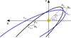Fig. 2. Displacement of the trajectory and time shifts of the exoplanet in-between two approximate successive Keplerian orbits N − 1 and N. The two main contributions δtk and δtP of the (rough) estimation of the time shift are indicated. The point $T_{N-1}^{\prime }$ is the point corresponding to TN − 1 reported in the next orbit N.

The first delay is due to the different orientation of the Nth Keplerian ellipse with respect to the (N − 1)th one, shifted by the relativistic precession angle ω_N − ω_N − 1 ≃ 2πk (see Fig. A.1). It simply reads n₀ δt_k ≃ ℓ_N − ℓ_N − 1, where n₀ is the Newtonian mean motion and ℓ_N the mean anomaly solving the transit condition of the Nth orbit (for a given transit T_i or eclipse ${\overline{T}}_i$). Of course the mean anomaly is counted from the periastron P_N of the Nth orbit, and is given in terms of the eccentric anomaly by Kepler’s equation ℓ_N = ψ_N − e sin ψ_N. The condition relating the corresponding true anomalies of the successive ellipses is thus

$$\begin{array}{c}\hfill arctan(\sqrt{\frac{1+e}{1-e}}tan\frac{{\psi }_N}{2})-arctan(\sqrt{\frac{1+e}{1-e}}tan\frac{{\psi }_{N-1}}{2})+\pi k\simeq 0.\end{array}$$(A.1)

As for the second time delay, it is due to the modification of the mean motion (and thus the period) as given by n = n₀(1 + ζ) (see Eq. (19a)). We have ℓ = n₀(t − t_PN), which we can roughly equate to n(t − t_PN − 1), where t_PN − 1 and t_PN are the successive instants of passage at periastron. Thus t_PN − t_PN − 1 ≃ −ζ(t − t_PN − 1), and we roughly approximate t − t_PN − 1 by the period so that n₀ δt_P ≃ −2πζ. The time delay between the Nth orbit and the reference one finally becomes

$$\begin{array}{c}\hfill \delta t(N)\simeq \frac{{\psi }_N-{\psi }_0-e(sin{\psi }_N-sin{\psi }_0)-2\pi N\zeta }{n_0}·\end{array}$$(A.2)

References

- Blanchet, L. 2014, Liv. Rev. Relativ., 17, 2 [Google Scholar]
- Blanchet, L., & Iyer, B. R. 2003, Class. Quant. Grav., 20, 755 [NASA ADS] [CrossRef] [Google Scholar]
- Blanchet, L., & Novak, J. 2011, MNRAS, 412, 2530 [NASA ADS] [CrossRef] [Google Scholar]
- Brouwer, D., & Clemence, G. 1961, Methods of Celestial Mechanics (New York: Academic Press) [Google Scholar]
- Correia, A. C. M., Laskar, J., Farago, F., & Boué, G. 2011, Celest. Mech. Dyn. Astron., 111, 105 [Google Scholar]
- Damour, T., & Deruelle, N. 1985, Ann. Inst. H. Poincaré Phys. Théor., 43, 107 [Google Scholar]
- Damour, T., & Esposito-Farèse, G. 1994, Phys. Rev. D, 49, 1693 [NASA ADS] [CrossRef] [Google Scholar]
- de Wit, J., Lewis, N. K., Langton, J., et al. 2016, ApJ, 820, L33 [NASA ADS] [CrossRef] [Google Scholar]
- Fabrycky, D. 2010, in Non-Keplerian Dynamics of Exoplanets, ed. S. Seager (Tucson: The University of Arizona Press), 217 [Google Scholar]
- Figueira, P., Santerne, A., Suárez Mascareño, A., et al. 2016, A&A, 592, A143 [NASA ADS] [CrossRef] [EDP Sciences] [Google Scholar]
- Fossey, S. J., Waldmann, I. P., & Kipping, D. M. 2009, MNRAS, 396, L16 [NASA ADS] [CrossRef] [Google Scholar]
- Garcia-Melendo, E., & McCullough, P. R. 2009, ApJ, 698, 558 [NASA ADS] [CrossRef] [Google Scholar]
- Gilvarry, J. J. 1953, Phys. Rev., 89, 1046 [NASA ADS] [CrossRef] [Google Scholar]
- Gimenez, A. 1985, ApJ, 405, 167 [Google Scholar]
- Gradshteyn, I., & Ryzhik, I. 1980, Table of Integrals, Series and Products (New York: Academic Press) [Google Scholar]
- Hébrard, G., Desert, J.-M., Diaz, R. F., et al. 2011, A&A, 516, A95 [Google Scholar]
- Heyl, J. S., & Gladman, B. J. 2007, MNRAS, 377, 1511 [NASA ADS] [CrossRef] [Google Scholar]
- Hidas, M. G., Tsapras, Y., Street, R. A., et al. 2010, MNRAS, 406, 1146 [NASA ADS] [Google Scholar]
- Hulse, R., & Taylor, J. 1975, ApJ, 195, L51 [NASA ADS] [CrossRef] [Google Scholar]
- Iorio, L. 2011, MNRAS, 411, 167 [NASA ADS] [CrossRef] [Google Scholar]
- Jordàn, A., & Bakos, G. 2008, ApJ, 685, 543 [NASA ADS] [CrossRef] [Google Scholar]
- Kramer, M., Stairs, I. H., Manchester, R. N., et al. 2006, Science, 314, 97 [NASA ADS] [CrossRef] [PubMed] [Google Scholar]
- Laughlin, G., Deming, D., Langton, J., et al. 2009, Nature, 457, 562 [NASA ADS] [CrossRef] [PubMed] [Google Scholar]
- Moutou, C., Hébrard, G., Bouchy, F., et al. 2009, A&A, 498, L5 [NASA ADS] [CrossRef] [EDP Sciences] [Google Scholar]
- Naef, D., Latham, D. W., Mayor, M., et al. 2001, A&A, 375, L27 [NASA ADS] [CrossRef] [EDP Sciences] [Google Scholar]
- O’Toole, S. J., Tinney, C. G., Jones, H. R. A., et al. 2009, MNRAS, 392, 641 [NASA ADS] [CrossRef] [Google Scholar]
- Pàl, A., & Kocsis, B. 2008, MNRAS, 389, 191 [NASA ADS] [CrossRef] [Google Scholar]
- Parsa, M., Eckart, A., Shahzamanian, B., et al. 2017, ApJ, 845, 22 [NASA ADS] [CrossRef] [Google Scholar]
- Pont, F., Hebrard, G., Irwin, J. M., et al. 2009, A&A, 502, 695 [NASA ADS] [CrossRef] [EDP Sciences] [Google Scholar]
- Roberts, J. E., Barnes, J. W., Rowe, J. F., & Fortney, J. F. 2013, ApJ, 762, 55 [NASA ADS] [CrossRef] [Google Scholar]
- Shporer, A., Winn, J. N., Dreizler, S., et al. 2010, ApJ, 722, 880 [NASA ADS] [CrossRef] [Google Scholar]
- Taylor, J., & Weisberg, J. 1982, ApJ, 253, 908 [NASA ADS] [CrossRef] [Google Scholar]
- Wagoner, R., & Will, C. 1976, ApJ, 210, 764 [NASA ADS] [CrossRef] [Google Scholar]
- Will, C. M. 1993, Theory and Experiment in Gravitational Physics (Cambridge: Cambridge University Press) [CrossRef] [Google Scholar]
- Winn, J. N., Howard, A. W., Johnson, J. A., et al. 2009, ApJ, 703, 2091 [NASA ADS] [CrossRef] [Google Scholar]
- Wolf, M., Claret, A., Kotková, L., et al. 2010, A&A, 509, A18 [NASA ADS] [CrossRef] [EDP Sciences] [Google Scholar]