| Issue |
A&A
Volume 628, August 2019
|
|
|---|---|---|
| Article Number | A107 | |
| Number of page(s) | 6 | |
| Section | Stellar atmospheres | |
| DOI | https://doi.org/10.1051/0004-6361/201935654 | |
| Published online | 14 August 2019 | |
Magnetic activity of the solar-like star HD 140538
1
Hamburger Sternwarte, Universität Hamburg,
Gojenbergsweg 112,
21029
Hamburg,
Germany
e-mail: This email address is being protected from spambots. You need JavaScript enabled to view it.
2
Space Science Institute,
4750 Walnut Street, Suite 205,
Boulder,
CO
80301,
USA
3
Max-Planck-Institut für Sonnensystemforschung,
Justus-von-Liebig-Weg 3,
37077
Göttingen,
Germany
4
Department of Astronomy, University of Guanajuato,
Guanajuato,
Mexico
5
Sterrewacht Leiden, University of Leiden,
Leiden,
The Netherlands
Received:
10
April
2019
Accepted:
28
June
2019
Abstract
The periods of rotation and activity cycles are among the most important properties of the magnetic dynamo thought to be operating in late-type, main-sequence stars. In this paper, we present a SMWO-index time series composed from different data sources for the solar-like star HD 140538 and derive a period of 3.88 ± 0.02 yr for its activity cycle. Furthermore, we analyse the high-cadence, seasonal SMWO data taken with the TIGRE telescope and find a rotational period of 20.71 ± 0.32 days. In addition, we estimate the stellar age of HD 140538 as 3.7 Gyrs via a matching evolutionary track. This is slightly older than the ages obtained from gyrochronology based on the above rotation period, as well as the activity-age relation. These results, together with its stellar parameters that are very similar to a younger Sun, make HD 140538 a relevant case study for our understanding of solar activity and its evolution with time.
Key words: stars: atmospheres / stars: activity / stars: chromospheres / stars: late-type / stars: individual: HD 140538 / stars: rotation
© ESO 2019
1 Introduction
By diligently counting the number of sunspots on the surface of the Sun, Schwabe (1844) discovered the eleven-year solar activity cycle, which has hitherto been observed in many observational indicators over almost the entire electromagnetic spectrum. Since stars cannot be spatially resolved, Schwabe’s technique cannot be applied, and other methods must be used, for example, monitoring the cores of the Ca II H&K lines. Eberhard & Schwarzschild (1913) were the first to note, on accidentally overexposed plates, “extraordinarily bright, sharp emission lines in the middle” (Eberhard & Schwarzschild 1913, p.292, ll. 25-26) of the Ca II H&K lines – among others – in the star σ Gem, an active RS CVn binary system, and interpreted these reversals as “The same kind of eruptive activity that appears in sun-spots, flocculi, and prominences” (Eberhard & Schwarzschild 1913, p.294, ll. 33-34) known from the Sun. It is remarkable that Eberhard & Schwarzschild (1913) already considered using the core emission as cycle diagnostics and wrote that “It remains to be shown whether the emission lines of the star have a possible variation in intensity analogous to the sun-spot period.” (Eberhard & Schwarzschild 1913, p.295, ll. 3-5).
This idea was taken up in 1966, when O.C. Wilson started the famous Mount Wilson project with a specially designed HK photometer (Wilson 1978; Vaughan et al. 1978). Over more than three decades a systematic search for stellar activity cycles based on the so-called S-index, which measures the strength of Ca II H&K emission lines, was carried out. Baliunas et al. (1995) present the Mount Wilson project results for 112 stars (including the Sun), with 46 stars showing evidence of an activity cycle.
After the official end of the Mount Wilson programme, other programmes continued Ca II H&K monitoring with spectroscopic means. Lowell Observatory (Hall & Lockwood 1995; Hall et al. 2007) used the Solar-Stellar Spectrograph (SSS) to this end, but their observations do not cover all objects listed in Baliunas et al. (1995). In the last twenty years, other Ca II H&K monitoring programmes were carried out, often in the context of radial velocity searches for extrasolar planets, where S-indices can be derived as a by-product. Catalogues of S-indices are published by see e. g., Henry et al. (1996); Gray et al. (2003); Isaacson & Fischer (2010).
At Hamburg Observatory we continued Ca II H&K monitoring in 2013, including all stars listed in Baliunas et al. (1995), using our robotic spectroscopy telescope TIGRE (Telescopio Internacional de Guanajuato, Robótico-Espectroscópico) (Schmitt et al. 2014), located at La Luz Observatory in central Mexico. Stars listed in Hall et al. (2007) are also part of the TIGRE activity survey target list to obtain an overlap between the Ca II H&K programmes at Lowell and Hamburg Observatories. To obtain a longer time span and to increase data density, the Ca II H&K measurements from different sources can be combined, and in this fashion Metcalfe et al. (2013) found two activity cycles in ɛ Eri, which were not listed as cyclic by Baliunas et al. (1995).
The wider scope of this research is to study solar magnetic activity by means of younger and older, very sun-like stars. Since the sample of such stars with known activity cycles and rotation periods is still quite small, any new addition to it is very valuable. The relation between the period of an activity cycle and the rotation is particularly relevant in this context, because it provides important information about the magnetic dynamo thought to be operating in the Sun and solar-like stars (Metcalfe & van Saders 2017). Therefore, the search of new activity cycles is an important task to better understand and characterise stellar dynamos. In this paper, we present a combined Ca II H&K time series of the solar-like star HD 140538 and the results of our cycle analysis. We also report a measurement of the rotation period of HD 140538, based on high-cadence seasonal data taken with the TIGRE telescope, and then estimate the age of HD 140538, based on the independentmethods of evolutionary tracks, gyrochronology, and activity.
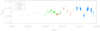 |
Fig. 1 Combined SMWO time series. The individual time series are colour-coded and labelled with different symbols (Keck: green asterisks, SMARTS: red diamonds, SSS: black crosses, and TIGRE: blue triangles). |
2 Physical parameters of HD 140538
HD 140538 (= ψ Ser) is a bright (5.86 mag) G2.5 main-sequence star with a rotational velocity v sin (i) of 1.58 ± 0.13 km s−1 (dos Santos et al. 2016) at a distance of 14.77 ± 0.01 pc (Gaia Collaboration 2018) and a colour index of B − V = 0.684 ± 0.002 mag (ESA 1997). From this brightness and distance an absolute visual magnitude of 5.013 ± 0.002 mag can be deduced. Using the PASTEL catalogue (version 2016-05-02; Soubiran et al. 2016), we computed the median of the listed log(g), [Fe/H], and Teff values without double recorded values. Furthermore, standard deviations of each median are computed from the median absolute deviation and assumed these values as the uncertianty of the parameters. We obtain for log(g) a median of 4.46 ± 0.06, for [Fe/H] a median of 0.05 ± 0.02, and for Teff a median of 5683 ± 15 K. A comparison of these values with the solar values shows HD 140538 to be slightly cooler and its metallicity to be slightly higher, but overall the stellar parameters of HD 140538 are very close to those for the Sun, suggesting that HD 140538 is (close to being) a solar twin. On the other hand, Mahdi et al. (2016) provide a study with a list of solar twin candidates that includes HD 140538,but they find differences in abundance and age compared to the Sun, and consequently do not include HD 140538 in their final list of solar twin stars.
3 Monitoring chromospheric activity by S-index data
To study the long-term chromospheric activity of HD 140538, we used the SMWO values from four different data sources and combine all the available data into a single data set with a total of 438 individual SMWO measurements over the time period of 1997 to now. Our time series is displayed in Fig. 1. In the following we briefly describe the individual data sets.
3.1 Keck
We used the SMWO-values from the catalogue published by Isaacson & Fischer (2010), who provide SMWO time series for more than 2600 stars. These S-values were obtained in the context of the California Planet Search (CPS) programme with telescopes at the Keck and Lick Observatories. For our combined time series, we use only the S-index values obtained from the spectra taken at the Keck Observatory, since the Lick data show a rather large scatter. We use a total of 136 SMWO-values taken between 2004 to 2012.
3.2 SMARTS
To bridge the gap between the measurements from Keck and TIGRE, we used observations from the SMARTS southern HK project (Metcalfe et al. 2010, 2013). These data include 45 low-resolution (R ~ 2500) spectra obtained at 23 epochs between February 2008 and July 2012 using the RC Spec instrument on the 1.5-m telescope at Cerro Tololo Interamerican Observatory. Bias and flat-field corrections were applied to the 180 s integrations, and the wavelength was calibrated using standard IRAF routines. SMWO values were extracted from the reduced spectra following Duncan et al. (1991), placing the instrumental measurements onto the Mount Wilson scale from contemporaneous observations of 26 stars from the SSS.
3.3 Solar-Stellar Spectrograph
We use SMWO data from the SSS published by Radick et al. (2018). It should be noted that these data are seasonal or rather yearly S-values covering a time span of20 yr from 1995 to 2016, constituting the longest individual time series in our data set. The total number of individual S-index values in a single season varies between 8 values (in 2008) and 38 values (in 2009), with an average of 24 S-index values per season.
3.4 TIGRE
We finally used our own TIGRE S-indices estimated from spectra taken with the fully robotic TIGRE telescope. The TIGRE telescope has an aperture of 1.2 m and its only instrument is the two spectral channel fibre-fed échelle spectrograph HEROS (Heidelberg Extended Range Optical Spectrograph) with a spectral resolution of R ≈ 20000 covering the wavelength range between 3800 and 8800 Å with a small gap between the two spectral channels; a more detailed description of the TIGRE telescope is given by Schmitt et al. (2014). The estimation of the instrumental TIGRE S-index and its transformation onto the Mount Wilson scale is described by Mittag et al. (2016). The total number of TIGRE spectra used is 238, covering the time span between 2014 and 2019.
3.5 Combined S-index time series
When combining the four individual data sets into a single data set, we had to consider possible offsets of individual data sets caused by small differences in the calibration into the Mount Wilson scale. This expected misalignment was visible and had to be corrected. For that, we used the SSS data as a reference and re-scaled the other three data sets to the scale of the SSS data. To re-scale the time series, the mean of the S-values of the time series in the time overlap regions were computed, and the ratio between the mean value of the SSS data and the other time series was used as scaling factor. In Table 1, we list the number of SMWO values, the mean re-scaled SMWO, the standard deviation, the log  (Mittag et al. 2013), and the scale factor for each individual time series. The combined and corrected time series is displayed in Fig. 1. The individual time series are colour-coded and labelled with different symbols.
Data sets, number of SMWO values, mean re-scaled SMWO, standard deviation (σ), corresponding log  for each timeseries and re-scaling factor.
4 Magnetic activity: cycle, rotation, and age
In this section we present the results of our investigation of the stellar activity based on the combined SMWO time series of HD 140538,and also discuss the general chromospheric and coronal activity level of HD 140538. We performed a Lomb-Scargle analysis of the SMWO time series to estimate the activity cycle, and discuss a possible rotational period found in the TIGRE data.
4.1 Chromosphere
HD 140538 is listed in the Washington Double Star Catalogue (Mason et al. 2001) with five individual components. However, these are much fainter than the main object so that for the S-index, the influence of these additional components is negligible. The individual SMWO time series all have a different number of data points. Therefore, we calculated the mean SMWO values for each individual corrected time series and list these values in Table 1. The values in Table 1 yield a mean SMWO of 0.228 with a standard deviation of 0.008. Given that HD 140538 is close to being a solar twin, we can directly compare the activity level of HD 140538 with the chromospheric activity level of the Sun. Using a mean solar SMWO-value of 0.1694 ± 0.0005 (Egeland et al. 2017), we estimate a ≈35% higher chromospheric activity level of HD 140538 compared to the Sun.
4.2 X-ray emission
HD 140538 has apparently never been the target of a dedicated X-ray observation according to the archives of the XMM-Newton and ROSAT missions. However, X-ray emission from HD 140538 has been detected in the context of the ROSAT all-sky survey (RASS). Inspecting the catalogue of RASS X-ray sources by Boller et al. (2016), we identify the X-ray source 2RXS J154402.0 + 023054 with HD 140538. Boller et al. (2016) report 2RXS J154402.0 + 023054 with a count rate of 0.15 ± 0.02 cts s−1. The positional coincidence and the softness of the recorded spectrum make this identification essentially certain; no indications of time variability are found in the RASS data.
Using the count-rate-to-flux conversion by Schmitt et al. (1995) we find an apparent soft X-ray flux of 7.3 × 10⁻¹³ erg cm−2 s−1, which translates into an X-ray luminosity of 1.9 × 1028 erg s−1, using a distance of 14.77 pc (Gaia Collaboration 2018). Thus, although very similar to the Sun in a variety of aspects, HD 140538 exceeds the X-ray output of the active Sun by at least an order of magnitude, which is in line with its likewise enhanced chromospheric activity.
4.3 Activity cycle
A visual inspection of the S-index time series of HD 140538 shows a clear approximately four-year periodic variation, which was already noted by Hall et al. (2007). An extended time series of SSS S-index values is shown by Hall et al. (2009) and Radick et al. (2018). Here we perform a rigorous period analysis based on the Lomb-Scargle periodogram.
For this analysis, we used the generalised Lomb-Scargle (GLS) formalism by Zechmeister & Kürster (2009). This formalism is based on a χ2 minimisation with the model y(t) = a sin(ωt) + b cos(ωt) + c, where c is a constant. Therefore, the peak of the periodogram provides not only the probability of the period, it is also a sign of the quality of the χ2 fit by the given period. To estimate the error of the period, we used the error equation for the period from Baliunas et al. (1995, Eq. (3)).
The SSS S-index values published by Radick et al. (2018) show a slightly increasing trend, which is also visible in the combined S-index time series. This may be an indication of a long-term activity cycle. However, we performed a Lomb-Scargle analysis without the removal of this trend to test its influence on the period estimation. The periodogram is shown as a dotted line in Fig. 2c, and we find a clear peak at the period of 3.91 ± 0.02 yr. The peak height is 0.495, which corresponds to a formal FAP (false alarm probability) of 4 × 10−62, in other words, this periodicity is very certain. The sinusoidal fit is shown in Fig. 2a as a dotted line. It can be seen that the fit is systematically higher for the data before 2005. In the next step, we removed this trend from the S-index data because the trend is not considered in the GLS formalism and could have an influence on the period estimation.
For the trend estimation, we used only the seasonal SSS S-index values because these data are the most homogeneous and form longest set of our four data sets. For the seasons from 2017 to 2019, we extended the SSS data with the seasonal TIGRE S-index values from 2017. In Fig. 2a, these seasonal values are shown as red asterisks with all S-index values as black crosses. For the trend, we use a linear approach and the result of the fit is plotted in Fig. 2a as a solid line. After removing the trend (see Fig. 2b), we perform a Lomb-Scargle analysis, using GLS formalism. The periodogram of this analysis is shown in Fig. 2c. We find a clear signal with a period of 3.88 ± 0.02 yr, a peak height of 0.588, and a corresponding formal FAP of 2 × 10−81, which is higher than without the trend removal. This is also an indication for a trend in the data because the GLS model fits better after the removal of the trend. This is visible in Fig. 2 when comparing both fits. Therefore, we prefer the period obtained after the trend removal. On the other hand, both periods are equal within the error and this shows that de-trending has only a very small effect on the period estimation. The possible reason is that the majority of data points are taken after 2005, so that the influence of the trend on the period estimation and the data before 2005 is small.
Independent of the de-trending, the period of the last cycle of this time series is shorter than in the other cycles, which we roughly estimate at a period of ≈3.4 yr. Therefore, the data do not follow the sinusoidal fit with the 3.88-yr period. To test the influence of the last shorter cycle on the 3.88-yr period, we estimated the period without this cycle and obtained a period of 3.99 ± 0.02 yr with a formal FAP of 1 × 10−88. However, period variations of ≈10% are known to occur from the well-studied solar cycle, so this may already explain the discrepancy.
In the plot of the residuals (see Fig. 2b) a negative trend starting in about 2015 can be observed. This could indicate that the cycle maximum of the possibly longer term cycle has passed and the activity is decreasing slowly to the next minimum of the longer term cycle. To verify this, we need longer observations. However, if this true, half of the long-term cycle can be seen under the additional assumption that at the beginning of the time series, the star was in the minimum of this long-term cycle. Therefore, a period of this long-term cycle can be roughly estimated at around 30 yr.
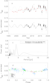 |
Fig. 2 Panel a: combined SMWO time series is displayed with black crosses. The red asterisks show the seasonal data from SSS and TIGRE data and the solid line the result of the linear trend fit. The dotted line depicts the sinusoidal fit of the Lomb-Scargle analysis of the non-detrended data with a period of 3.91 yrs. Panel b: detrended SMWO time series. The solid line represents the sinusoidal fit with the period of 3.88 yr found in the GLS analysis. Panel c: periodograms of GLS (generalised Lomb-Scargle) analysisof detrended and non-detrended data. Panel d: phase-folded detrended SMWO time series shown with sinusoidal fit. Here, the SMWO of the individual time series are colour-coded and labelled (Keck: green asterisks, SMARTS: red diamonds, SSS: black crosses, and TIGRE: blue triangles). |
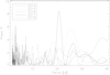 |
Fig. 3 Periodograms of GLS analysis for each TIGRE observation season. The years are shown in the following manner: 2014 by a dashed-single-dotted line; 2015 a dotted line; 2016 a dashed line; 2017 a solid line; 2018 a dashed-triple-dotted line. |
4.4 Rotation period
The rotation period of a star is a key parameter to characterise its stellar activity. Our TIGRE measurements are sufficiently densely sampled to allow meaningful period measurements. In Fig. 3 we show the GLS periodograms ( ), including the noise level for each observational season, the individual seasons are shown with different line styles. Somewhat surprisingly, only in the season of 2017 could we find a significant rotational period at 20.71 ± 0.32 days (see Fig. 3). The formal FAP of this peak is 0.007 with a significance of 99.3%. The upper panel of Fig. 4 shows the TIGRE SMWO values recorded in the 2017 season, where the two values plotted in red are treated as outliers and thus ignored in the GLS analysis. The solid line depicts the sinusoidal fit with the determined rotational period. In addition, the phased-folded TIGRE SMWO values for this 2017 season are shown with the best sinusoidal fit as a solid line in the lower panel of Fig. 4.
Furthermore, we were able to use the estimated mean SMWO-index of 0.228 to calculate the rotational period from the activity-rotation relation. First, we converted the mean SMWO-index of 0.228 into the  value using the conversion developed by Mittag et al. (2013) and obtain
  = 2.18 ± 0.22. From that, we estimated the Rossby number of 0.5 from the activity-rotation relation developed by Mittag et al. (2018). With this Rossby number and the convective turnover time used in Mittag et al. (2018), we calculated a rotational period of 21.3
 days for HD 140538 in good agreement with our TIGRE measurements; we note that Isaacson & Fischer (2010) also arrived a rotational period of about 20 days. The comparison with the calculated periods shows that the rotational period obtained from the TIGRE SMWO-index time series are reasonable although the significance of the results is slightly lower than the formal 3σ level.
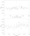 |
Fig. 4 Upper panel: TIGRE SMWO-index values of 2017 season with two outliers plotted as red data points. The solid line shows the sinusoidal fit with the 20.71 days rotational period. Lower panel: phase-folded SMWO -index time series shown with rotational period of 20.71 days. The solid line depicts the best sinusoidal fit. |
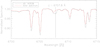 |
Fig. 5 Comparison of the co-added spectrum of HD 140538 (black line) and co-added solar spectrum (red line). |
4.5 Stellar age
In the context of gyrochronology, stellar rotation is directly related to stellar age (Barnes 2007), and, in a wider context, to the evolutionarystage of the star (see, among a vast literature, Schröder et al. 2013 and references therein). Despite stellar age being such an important stellar parameter, it is rather difficult to determine in absolute terms. Here we use different methods to assess the likely age of HD 140538.
We firstinspect our TIGRE spectra for the presence of the lithium line at 6707.8 Å. In Fig. 5 we show the co-added TIGRE spectra of HD 140538 (black line) and the Sun (measured from Moon light spectra, indicated by the red line), where the clear presence of lithium absorption in contrast to the Sun is observable. While actual lithium “clocks” are quite controversial, we conclude that HD 140538 is younger than the Sun, as expected from its faster rotation.
We nextused evolutionary tracks to quantitatively determine the age of HD 140538. To that end we used the evolutionary tracks with the Cambridge Stellar Evolution Code1 (Pols et al. 1997), which is an updated version of the evolution code written by Eggleton (1971). The code requires values for stellar mass and metallicity as input parameters. As a first step it is necessary to fine-calibrate the code with the solar values. Here we used the empirical calibration from Mittag et al. (2016) and plot the resulting evolutionary track (as a solid line), as well as the position of the Sun (as a filled circle) in the Hertzsprung–Russell diagram (HRD). This model is calculated with Z = 0.0185 ([Fe/H] = 0.00) and suggests a solar age of around 4.6 Gyr, which is consistent with the age obtained by Bouvier & Wadhwa (2010).
Using the absolute visual magnitude of 5.013 ± 0.002 mag and the bolometic correction (BC) of −0.12 mag calculated from Gray (2005, Eq. (10.9)), we find a luminosity of log L ∕ L⊙ = −0.061, ± 0.001 for HD 140538 with Mbol,⊙ = 4.74 mag (Cox 2000). With this value and an effective temperature of Teff of 5683 ± 15 K, the position of HD 140538 in the HRD is well defined and shown as an asterisk in Fig. 6; note that the parallax error of HD 140538 is very small and thus negligible for the age estimation. The uncertainty in Teff also influences the stellar age estimate since a variation in stellar mass and the uncertainty in metallicity causes a shift in the effective temperature. To consider these variations, we estimated the stellar age for Teff ± 15 K with fixed metallicity by variation of the stellar mass. Furthermore, we estimated the stellar age and mass of the best-matching tracks for Z = 0.0208 ± 0.001, which is the corresponding the error range of the metallicity. The evolutionary track for HD 140538 is then calculated with M = 1.009 M⊙ and Z = 0.0208 and depicted as a dashed line in Fig. 6. This evolutionary track suggests 3.7 ± 1.6 Gyr as the likely stellar age of HD 140538, and we estimate a stellar mass of M = 1.01 ± 0.02 M⊙. These results show that HD 140538 is younger than our Sun with a mass that is possibly slightly higher.
In addition, we estimated the age of HD 140538 from the mean activity of HD 140538 and the rotation period of this star derived in Sects. 4.1 and 4.4. To obtain the age from the rotation, we used the method of gyrochronology following Barnes (2007) and calculated an age of 2.4 ± 0.3 Gyr. From the activity, we calculated an age of 2.2 ± 0.3 Gyr with the age-activity relation derived by Mamajek & Hillenbrand (2008) and a  of −4.72 using the transformation equations from SMWO into
  from Noyes et al. (1984). Both ages are consistent with the stellar age to within the error obtained from the evolutionary track.
Finally, we checked the catalogues in the Simbad/VizieR database to find other age estimates. Mamajek & Hillenbrand (2008) list HD 140538 with an age of 3.2 Gyr and a  of −4.80 taken from Hall et al. (2007), while Casagrande et al. (2011) quote an age of 0.3 Gyr and Takeda et al. (2007) an age of 7.72 Gyr. Given the activity properties of HD 140538, the latter two age estimates appear quite unlikely, while the age estimated by Mamajek & Hillenbrand (2008) is obviously consistent with our estimates.
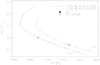 |
Fig. 6 Luminosity vs. effective temperature of the stars. The solid line shows the evolutionary track for 1.00 M⊙ with Z = 0.0185 and the dashed line for 1.009 M⊙ with Z = 0.0208. The diamonds on the evolutionary track mark time steps of 1 Gyr, with the first marked time step at 1 Gyr and at 2 Gyr, respectively. |
5 Discussion and conclusion
In this work,we combined the SMWO measurements from the SSS project, Keck data (CPS), SMARTS data (southern HK project) and TIGRE data to study the magnetic activity of HD 140538. In our long-term time series we find a clear activity cycle with a cycle period of 3.88 ± 0.02 yr. In each individual data set, this variation is also clearly visible, however, the time series also shows a long-term trend that might be an indication for a long-term activity cycle. With the derived activity cycle period of 3.88 yr and the rotational period of 20.71 day, HD 140538 fits very well in the Pcyc vs. Prot distribution for stars on the short, inactive branch shown in Brandenburg et al. (2017, Fig. 4).
The mean SMWO-index of HD 140538 of 0.228 is clearly larger than the mean S-value of the Sun with 0.1694 (Egeland et al. 2017), and the X-ray luminosity obtained with ROSAT shows HD 140538 to be far more active than our Sun. In our seasonal TIGRE data, we find a weak periodic signal at a period of 20.71 day with a significance of 99.3%, which we interpret as the rotational period of HD 140538. All this evidence points to a star younger than the Sun, and indeed our age estimates result in values less than the solar age, independently of whether ages based on age-activity relations, gyrochonological ages, or evolutionary ages are considered.
Inspecting our long-term time series it appears that in the early 1990s HD 140538 was in a minimum of the above long-term cycle. The cycle amplitude also seems to have changed, with amplitude variations of the 3.88 yr cycle becoming stronger with time. Comparable behaviour in the short-term cycle was also observed in the ɛ Eri time series published by Metcalfe et al. (2013): in ɛ Eri the periodic variations caused by the short-term cycle were not visible during the minimum of the long-term cycle behaviour (Metcalfe et al. 2013) assumed to be caused by two different dynamos producing the two cycle branches shown in Böhm-Vitense (2007).
Since the stellar parameters of HD 140538 are very close to those of the Sun, but HD 140538 has three-quarters of the solar age, HD 140538 presents a very good case in the context of the Sun-in-time theme. Further S-index monitoring of HD 140538 is necessary to find and measure the suspected longer cycle period (expected from the combined S-index time series and from the long-period branch; Brandenburg et al. 2017) from an entire, longer time series. Since the cycle timescales in HD 140538 are three times shorter than in the case of the Sun (which is a Schwabe cycle of eleven years, a long-period cycle is possibly the Gleisberg cycle of about a century), we expect a period of about thirty years, which requires patience and stamina to measure.
Acknowledgements
We thank the referee, Ricky Egeland, for the helpful comments and suggestions. T.S.M. acknowledges support from a Visiting Fellowship at the Max Planck Institute for Solar System Research. The authors from Hamburg and Guanajuato are grateful for financial support from the Conacyt-DFG bilateral project No. 278 156, which enables us to intensify our collaboration by mutual visits. This research has made use of the VizieR catalogue access tool, CDS, Strasbourg, France (DOI: 10.26093/cds/vizier). The original description of the VizieR service was published in Ochsenbein et al. (2000).
References
- Baliunas, S. L., Donahue, R. A., Soon, W. H., et al. 1995, ApJ, 438, 269 [NASA ADS] [CrossRef] [Google Scholar]
- Barnes, S. A. 2007, ApJ, 669, 1167 [NASA ADS] [CrossRef] [Google Scholar]
- Böhm-Vitense, E. 2007, ApJ, 657, 486 [NASA ADS] [CrossRef] [Google Scholar]
- Boller, T., Freyberg, M. J., Trümper, J., et al. 2016, A&A, 588, A103 [NASA ADS] [CrossRef] [EDP Sciences] [Google Scholar]
- Bouvier, A., & Wadhwa, M. 2010, Nat. Geosci., 3, 637 [NASA ADS] [CrossRef] [Google Scholar]
- Brandenburg, A., Mathur, S., & Metcalfe, T. S. 2017, ApJ, 845, 79 [NASA ADS] [CrossRef] [Google Scholar]
- Casagrande, L., Schönrich, R., Asplund, M., et al. 2011, A&A, 530, A138 [NASA ADS] [CrossRef] [EDP Sciences] [Google Scholar]
- Cox, A. N. 2000, Allen’s Astrophysical Quantities 3 (New York: Springer) [Google Scholar]
- dos Santos, L. A., Meléndez, J., do Nascimento, J.-D., et al. 2016, A&A, 592, A156 [NASA ADS] [CrossRef] [EDP Sciences] [Google Scholar]
- Duncan, D. K., Vaughan, A. H., Wilson, O. C., et al. 1991, ApJS, 76, 383 [NASA ADS] [CrossRef] [Google Scholar]
- Eberhard, G., & Schwarzschild, K. 1913, ApJ, 38, 292 [NASA ADS] [CrossRef] [Google Scholar]
- Egeland, R., Soon, W., Baliunas, S., et al. 2017, ApJ, 835, 25 [NASA ADS] [CrossRef] [Google Scholar]
- Eggleton, P. P. 1971, MNRAS, 151, 351 [NASA ADS] [CrossRef] [Google Scholar]
- ESA 1997, The HIPPARCOS and TYCHO catalogues. Astrometric and Photometric Star Catalogues Derived from the ESA HIPPARCOS Space Astrometry Mission, ESA SP, 1200 [Google Scholar]
- Gaia Collaboration 2018, VizieR Online Data Catalog: I/345 [Google Scholar]
- Gray, D. F. 2005, The Observation and Analysis of Stellar Photospheres (Cambridge: Cambridge University Press) [CrossRef] [Google Scholar]
- Gray, R. O., Corbally, C. J., Garrison, R. F., McFadden, M. T., & Robinson, P. E. 2003, AJ, 126, 2048 [NASA ADS] [CrossRef] [Google Scholar]
- Hall, J. C., & Lockwood, G. W. 1995, ApJ, 438, 404 [NASA ADS] [CrossRef] [Google Scholar]
- Hall, J. C., Lockwood, G. W., & Skiff, B. A. 2007, AJ, 133, 862 [NASA ADS] [CrossRef] [Google Scholar]
- Hall, J. C., Henry, G. W., Lockwood, G. W., Skiff, B. A., & Saar, S. H. 2009, AJ, 138, 312 [NASA ADS] [CrossRef] [Google Scholar]
- Henry, T. J., Soderblom, D. R., Donahue, R. A., & Baliunas, S. L. 1996, AJ, 111, 439 [NASA ADS] [CrossRef] [Google Scholar]
- Isaacson, H., & Fischer, D. 2010, ApJ, 725, 875 [NASA ADS] [CrossRef] [Google Scholar]
- Mahdi, D., Soubiran, C., Blanco-Cuaresma, S., & Chemin, L. 2016, A&A, 587, A131 [NASA ADS] [CrossRef] [EDP Sciences] [Google Scholar]
- Mamajek, E. E., & Hillenbrand, L. A. 2008, ApJ, 687, 1264 [NASA ADS] [CrossRef] [Google Scholar]
- Mason, B. D., Wycoff, G. L., Hartkopf, W. I., Douglass, G. G., & Worley, C. E. 2001, AJ, 122, 3466 [Google Scholar]
- Metcalfe, T. S., & van Saders, J. 2017, Sol. Phys., 292, 126 [NASA ADS] [CrossRef] [Google Scholar]
- Metcalfe, T. S., Basu, S., Henry, T. J., et al. 2010, ApJ, 723, L213 [NASA ADS] [CrossRef] [Google Scholar]
- Metcalfe, T. S., Buccino, A. P., Brown, B. P., et al. 2013, ApJ, 763, L26 [NASA ADS] [CrossRef] [Google Scholar]
- Mittag, M., Schmitt, J. H. M. M., & Schröder, K.-P. 2013, A&A, 549, A117 [NASA ADS] [CrossRef] [EDP Sciences] [Google Scholar]
- Mittag, M., Schröder, K.-P., Hempelmann, A., González-Pérez, J. N., & Schmitt, J. H. M. M. 2016, A&A, 591, A89 [NASA ADS] [CrossRef] [EDP Sciences] [Google Scholar]
- Mittag, M., Schmitt, J. H. M. M., & Schröder, K.-P. 2018, A&A, 618, A48 [NASA ADS] [CrossRef] [EDP Sciences] [Google Scholar]
- Noyes, R. W., Hartmann, L. W., Baliunas, S. L., Duncan, D. K., & Vaughan, A. H. 1984, ApJ, 279, 763 [NASA ADS] [CrossRef] [Google Scholar]
- Ochsenbein, F., Bauer, P., & Marcout, J. 2000, A&AS, 143, 23 [NASA ADS] [CrossRef] [EDP Sciences] [Google Scholar]
- Pols, O. R., Tout, C. A., Schroder, K.-P., Eggleton, P. P., & Manners, J. 1997, MNRAS, 289, 869 [NASA ADS] [CrossRef] [Google Scholar]
- Radick, R. R., Lockwood, G. W., Henry, G. W., Hall, J. C., & Pevtsov, A. A. 2018, ApJ, 855, 75 [NASA ADS] [CrossRef] [Google Scholar]
- Schmitt, J. H. M. M., Fleming, T. A., & Giampapa, M. S. 1995, ApJ, 450, 392 [NASA ADS] [CrossRef] [Google Scholar]
- Schmitt, J. H. M. M., Schröder, K.-P., Rauw, G., et al. 2014, Astron. Nachr., 335, 787 [NASA ADS] [CrossRef] [Google Scholar]
- Schröder, K.-P., Mittag, M., Hempelmann, A., González-Pérez, J. N., & Schmitt, J. H. M. M. 2013, A&A, 554, A50 [NASA ADS] [CrossRef] [EDP Sciences] [Google Scholar]
- Schwabe, H. 1844, Astron. Nachr., 21, 233 [NASA ADS] [CrossRef] [Google Scholar]
- Soubiran, C., Le Campion, J.-F., Brouillet, N., & Chemin, L. 2016, A&A, 591, A118 [NASA ADS] [CrossRef] [EDP Sciences] [Google Scholar]
- Takeda, G., Ford, E. B., Sills, A., et al. 2007, ApJS, 168, 297 [NASA ADS] [CrossRef] [Google Scholar]
- Vaughan, A. H., Preston, G. W., & Wilson, O. C. 1978, PASP, 90, 267 [NASA ADS] [CrossRef] [Google Scholar]
- Wilson, O. C. 1978, ApJ, 226, 379 [NASA ADS] [CrossRef] [Google Scholar]
- Zechmeister, M., & Kürster, M. 2009, A&A, 496, 577 [NASA ADS] [CrossRef] [EDP Sciences] [Google Scholar]
All Tables
Data sets, number of SMWO values, mean re-scaled SMWO, standard deviation (σ), corresponding log for each timeseries and re-scaling factor.
All Figures
|
Fig. 1 Combined SMWO time series. The individual time series are colour-coded and labelled with different symbols (Keck: green asterisks, SMARTS: red diamonds, SSS: black crosses, and TIGRE: blue triangles). |
| In the text | |
|
Fig. 2 Panel a: combined SMWO time series is displayed with black crosses. The red asterisks show the seasonal data from SSS and TIGRE data and the solid line the result of the linear trend fit. The dotted line depicts the sinusoidal fit of the Lomb-Scargle analysis of the non-detrended data with a period of 3.91 yrs. Panel b: detrended SMWO time series. The solid line represents the sinusoidal fit with the period of 3.88 yr found in the GLS analysis. Panel c: periodograms of GLS (generalised Lomb-Scargle) analysisof detrended and non-detrended data. Panel d: phase-folded detrended SMWO time series shown with sinusoidal fit. Here, the SMWO of the individual time series are colour-coded and labelled (Keck: green asterisks, SMARTS: red diamonds, SSS: black crosses, and TIGRE: blue triangles). |
| In the text | |
|
Fig. 3 Periodograms of GLS analysis for each TIGRE observation season. The years are shown in the following manner: 2014 by a dashed-single-dotted line; 2015 a dotted line; 2016 a dashed line; 2017 a solid line; 2018 a dashed-triple-dotted line. |
| In the text | |
|
Fig. 4 Upper panel: TIGRE SMWO-index values of 2017 season with two outliers plotted as red data points. The solid line shows the sinusoidal fit with the 20.71 days rotational period. Lower panel: phase-folded SMWO -index time series shown with rotational period of 20.71 days. The solid line depicts the best sinusoidal fit. |
| In the text | |
|
Fig. 5 Comparison of the co-added spectrum of HD 140538 (black line) and co-added solar spectrum (red line). |
| In the text | |
|
Fig. 6 Luminosity vs. effective temperature of the stars. The solid line shows the evolutionary track for 1.00 M⊙ with Z = 0.0185 and the dashed line for 1.009 M⊙ with Z = 0.0208. The diamonds on the evolutionary track mark time steps of 1 Gyr, with the first marked time step at 1 Gyr and at 2 Gyr, respectively. |
| In the text | |
Current usage metrics show cumulative count of Article Views (full-text article views including HTML views, PDF and ePub downloads, according to the available data) and Abstracts Views on Vision4Press platform.
Data correspond to usage on the plateform after 2015. The current usage metrics is available 48-96 hours after online publication and is updated daily on week days.
Initial download of the metrics may take a while.