| Issue |
A&A
Volume 628, August 2019
|
|
|---|---|---|
| Article Number | A61 | |
| Number of page(s) | 31 | |
| Section | Galactic structure, stellar clusters and populations | |
| DOI | https://doi.org/10.1051/0004-6361/201935299 | |
| Published online | 08 August 2019 | |
Metallicity, temperature, and gravity scales of M subdwarfs⋆,⋆⋆
1
Instituto de Astrofísica de Canarias (IAC), Calle Vía Láctea s/n, 38200 La Laguna, Tenerife, Spain
e-mail: This email address is being protected from spambots. You need JavaScript enabled to view it.
2
Departamento de Astrofísica, Universidad de La Laguna (ULL), 38205 La Laguna, Tenerife, Spain
3
Univ. Lyon, ENS de Lyon, Univ. Lyon1, CNRS, Centre de Recherche Astrophysique de Lyon UMR5574, 69007 Lyon, France
4
Visiting Professor at the Instituto de Astrofísica de Canarias (IAC), La Laguna, Tenerife, Spain
5
Departmento de Astrofísica, Centro de Astrobiología (CSIC-INTA), ESAC Campus, Camino Bajo del Castillo s/n, 286922 Villanueva de la Cañada, Spain
6
Spanish Virtual Observatory, 28692 Villanueva de la Cañada, Spain
7
Main Astronomical Observatory of the National Academy of Sciences of Ukraine, Ukraine
8
Center for Astrophysics Research, University of Hertfordshire, College Lane, Hatfield, Hertfordshire AL10 9AB, UK
9
Center for Astrophysics and Space Science, University of California San Diego, La Jolla, CA 92093, USA
10
Georg-August-Universität Goettingen Institut für Astrophysik, Friedrich-Hund-Platz 1, 37077 Göttingen, Germany
Received:
18
February
2019
Accepted:
1
July
2019
Abstract
Aims. The aim of the project is to define metallicity/gravity/temperature scales for different spectral types of metal-poor M dwarfs.
Methods. We obtained intermediate-resolution ultraviolet (R ∼ 3300), optical (R ∼ 5400), and near-infrared (R ∼ 3900) spectra of 43 M subdwarfs (sdM), extreme subdwarfs (esdM), and ultra-subdwarfs (usdM) with the X-shooter spectrograph on the European Southern Observatory Very Large Telescope. We compared our atlas of spectra to the latest BT-Settl synthetic spectral energy distribution over a wide range of metallicities, gravities, and effective temperatures to infer the physical properties for the whole M dwarf sequence (M0–M9.5) at sub-solar metallicities and constrain the latest atmospheric models.
Results. The BT-Settl models accurately reproduce the observed spectra across the 450–2500 nm wavelength range except for a few regions. We find that the best fits are obtained for gravities of log (g) = 5.0–5.5 for the three metal classes. We infer metallicities of [Fe/H] = −0.5, −1.5, and −2.0 ± 0.5 dex and effective temperatures of 3700–2600 K, 3800–2900 K, and 3700–2900 K for subdwarfs, extreme subdwarfs, and ultra-subdwarfs, respectively. Metal-poor M dwarfs tend to be warmer by about 200 ± 100 K and exhibit higher gravity than their solar-metallicity counterparts. We derive abundances of several elements (Fe, Na, K, Ca, Ti) for our sample but cannot describe their atmospheres with a single metallicity parameter. Our metallicity scale expands the current scales available for mildly metal-poor planet-host low-mass stars. Our compendium of moderate-resolution spectra covering the 0.45–2.5 micron range represents an important resource for large-scale surveys and space missions to come.
Key words: subdwarfs / stars: low-mass / techniques: spectroscopic / infrared: stars
All observed spectra are available at the CDS via anonymous ftp to cdsarc.u-strasbg.fr (130.79.128.5) or via http://cdsarc.u-strasbg.fr/viz-bin/qcat?J/A+A/628/A61
Based on observations collected at the European Southern Observatory, Chile, under programmes 089.C-0140(A), 091.C-0264(A), 092.D-0600(A), and 093.C-0610(A).
© ESO 2018
1. Introduction
Mass, gravity, temperature, and metallicity constitute key parameters to understand the formation and evolution of all type of stars. M dwarfs represent the largest population of stars among members of the solar neighbourhood (Henry et al. 2006; Bochanski et al. 2010; Kirkpatrick et al. 2012) and have also become attractive targets to search for Earth-like planets (e.g. Nutzman & Charbonneau 2008; Quirrenbach et al. 2012; Sozzetti et al. 2014). While the metal content of solar-type stars can be measured with high accuracy (e.g. Adibekyan et al. 2012), the metallicity of M dwarfs is more difficult to ascertain due to the significant number of absorption bands (Kirkpatrick et al. 1999). Several groups have conducted complementary surveys to assess the metallicity of M dwarfs based on photometry and colours (Bonfils et al. 2005; Johnson & Apps 2009; Schlaufman & Laughlin 2010; Neves et al. 2012; Hejazi et al. 2015; Dittmann et al. 2016) or high-resolution spectra and spectral synthesis of multiple systems composed of a solar-type primary and an M dwarf secondary at optical and infrared wavelengths (Woolf & Wallerstein 2005, 2006; Bean et al. 2006; Woolf et al. 2009; Rojas-Ayala et al. 2010, 2012; Muirhead et al. 2012; Terrien et al. 2012; Önehag et al. 2012; Neves et al. 2013, 2014; Hejazi et al. 2015; Newton et al. 2015; Lindgren et al. 2016). These surveys usually focus on slightly metal-poor M dwarfs, with metallicities above −1.0 dex. An extension to lower metallicities is needed to complement the precise distances that the Gaia satellite (de Bruijne 2012) will provide for a great number of spectroscopically confirmed thick-disk and halo M dwarfs (Savcheva et al. 2014) and also to understand the role of metallicity on the molecules and dust grains present in the atmosphere of low-mass stars.
M subdwarfs (sdMs) are population II dwarfs that appear bluer than solar-metallicity stars due to the dearth of metals in their atmospheres (Baraffe et al. 1997). These stars exhibit thick-disk or halo kinematics, including high proper motions or large heliocentric velocities (Gizis 1997). They belong to the first generation of stars and are important tracers of the chemical enrichment history of the Galaxy. The original classification for sdMs and extreme sdMs (esdMs) developed by Gizis (1997) has been revised and extended by Lépine et al. (2007). A new class of subdwarfs has been added, the ultra-subdwarfs (usdMs). The new scheme is based on a parameter, ζTiO/CaH, which quantifies the weakening of the strength of the TiO band (in the optical) as a function of metallicity. Subdwarfs are easily distinguished from dwarfs with solar abundances because they exhibit stronger metal-hydride absorption bands (FeH, CrH) and metal lines (CaI, FeI) as well as blue infrared colours caused by collision-induced H2–H2 absorption (Gizis 1997; Lépine et al. 2007; Lodieu et al. 2017). An independent classification scheme based on metallicity, gravity, and temperature has been proposed for M dwarfs by Jao et al. (2008) and an extension to the L dwarf regime proposed by Kirkpatrick et al. (2014) and Zhang et al. (2017).
In this paper, we present moderate-resolution 0.45–2.5 μm spectroscopy of 15 sdMs, 16 esdMs, and 12 usdMs to infer their metallicities and Teff by direct comparison with the latest BT-Settl synthetic models (Allard et al. 2012). In Sect. 2 we present our sample of metal-poor M dwarfs drawn from the literature. In Sect. 3 we describe our spectroscopic observations. In Sect. 4 we introduce the BT-Settl models used to infer the physical parameters of metal-poor M dwarfs. In Sect. 5 we infer the spectral type-versus-metallicity/gravity/Teff relation of the three M dwarf metal classes and compare it to independent but complementary studies as well as solar-type M dwarfs. In Sect. 6 we discuss our results and the peculiarities of some of the spectra.
2. Sample selection
To select our sample of subdwarfs, we used the SDSS spectroscopic database which contains a wealth of high-quality spectra covering the 5000–9200 Å range at a spectral resolution of ∼2000. Hundreds of objects have been classified as sdMs, esdMs, or usdMs following the scheme developed by Lépine et al. (2007). This classification is publicly available through the SDSS archive and we have taken advantage of it to retrieve a large sample of low-metallicity M dwarfs.
We selected a sub-sample of low-metallicity stars which represent a sequence going from M0 to M9.5 from optical spectra. The objects were specifically chosen to be the (or among the) brightest of their subclass and be observable either in August or January from the southern hemisphere to achieve the best signal-to-noise ratio possible over a wide wavelength range. We completed our sample with LHS 377 (sdM7; Gizis 1997), observed with the same telescope/instrument but at higher spectral resolution (Rajpurohit et al. 2016). Our final sample contains 15 sdM0–sdM9.5, 16 esdM0.0–esdM8.5, and 12 usdM0.0–usdM8.5) with almost one object per spectral sub-type. We are missing the sdM7.5, sdM8, and sdM9 in the sdM, the esdM2.5 and esdM8 in the esdM sequence, and more usdMs (usdM1.5, usdM2, usdM3.0, usdM6.5, usdM7, and usdM8). We note that these targets were included in our original sample but were not observed during the ESO service runs. Table 1 lists their coordinates, optical SDSSi magnitudes, optical spectral types on the Lépine et al. (2007) scheme, dates of observations, mean airmass, exposure times in all three arms, and numbers of AB cycles for all 43 subdwarfs.
Logs of the VLT/X-shooter spectroscopic observations of M subdwarfs.
3. VLT/X-shooter spectroscopy
We carried out spectroscopy from the UV- to the K band with the X-shooter spectrograph (D’Odorico et al. 2006; Vernet et al. 2011) mounted on the Cassegrain focus of the Very Large Telescope (VLT) Unit 2. Observations were conducted in service mode by the European Southern Observatory (ESO) staff over the course of three semesters, between August 2012 and June 2014 (Table 1). The conditions at the time of the observations met the clear sky request, with an airmass less than 1.6, grey conditions, and a seeing better than 1.2 arcsec. We set the individual on-source integration times according to the magnitudes of the targets and used the multiple AB patterns to correct for the sky contribution (mainly) in the near-infrared (NIR). All observations were done with the slit oriented at parallactic angle. We list all the M subdwarfs observed with X-shooter in Table 1 along with a summary of the logs of the observations.
X-shooter is a multi wavelength cross-dispersed echelle spectrograph made of three arms covering the ultraviolet (UVB; 0.3–0.55 μm), visible (VIS; 0.55–1.0 μm), and NIR (1.0–2.48 μm) wavelength ranges simultaneously thanks to the presence of two dichroics splitting the light. The spectrograph is equipped with three detectors: a 4096 × 2048 E2V CCD44-82, a 4096 × 2048 MIT/LL CCID 20, and a 2096 × 2096 Hawaii 2RG for the UVB, VIS, and NIR arms, respectively. We set the read-out mode to 400k and low gain without binning. We used the 1.6 arcsec slit in the UVB, 1.5 arcsec in the VIS, and 1.2 arcsec NIR, yielding resolving powers of 3300 (9.9 pixels per full-width-half-maximum), 5400 (9.7 pixels per full-width-half-maximum), and 3900 (5.8 pixels per full-width-half-maximum) in the UVB, VIS, and NIR arms, respectively.
We ran the latest version of the X-shooter pipeline (2.8.0)1 on the raw data downloaded from the ESO archive with their associated raw calibration files from our three programmes: 089.C-0140(A), 091.C-0264(A), and 093.C-0610(A). All spectra have their instrumental signature removed, including bias and flat-field. The spectra are wavelength-calibrated, sky-subtracted and finally flux-calibrated. The output products include a 2D spectrum associated with a 1D spectrum. However, the optimal extraction of the 1D spectrum not being yet implemented in the version 2.8.0 of the pipeline, we extracted the UVB, VIS, and NIR spectra with the apsum task under IRAF (Tody 1986, 1993). We note that most of the targets have little flux in the UVB arm, resulting in low signal-to-noise ratio below 550 nm and very little flux (or no flux) below 400 nm. We corrected the VIS and NIR spectra for telluric bands/lines with the molecfit package distributed by ESO (Kausch et al. 2015; Smette et al. 2015)2 mainly because the telluric standards were not necessarily taken at the same airmass as our targets. The regions corrected are: 625–632, 686–696, 716–732, 758–770, 812–834, 893–920, 928–980 nm in the VIS arm and 1105–1220, 1253–1280, 1310–1510, 1730–1995, 2000–2035, 2045–2085, 2200–2470 nm in the NIR arm.
The final spectral energy distributions (SEDs) of sdMs, esdMs, and usdMs are displayed in figures in Appendix A. For display purposes, we shifted the observed spectra to the BT-Settl models because of the large velocities of our subdwarfs taking into account that the wavelength scale of models is in vacuum and the observed spectra in the air system (see Sect. 5). Our sample increases the sample of subdwarfs presented in Rajpurohit et al. (2016) by a factor of five and extends that recent work to the full sequence of the three metallicity classes of M subdwarfs. We will make all spectra publicly available through the late-type subdwarf archive3 (Lodieu et al. 2017).
4. BT-Settl synthetic spectra
To infer the range of physical parameters (gravities i.e. log (g), metallicities [M/H], and Teff) for our sequence of subdwarfs, we employed the BT-Settl models (Allard et al. 2003, 2007; Allard & Freytag 2010; Allard et al. 2012) available for retrieval at the webpage4 of France Allard. The BT-Settl models account for TiO (Plez 1998, 2008) and H2O (Barber et al. 2006) among other opacities using the Caffau et al. (2011) abundance values and mixing information for the CO5BOLD code (Steiner et al. 2007; Freytag et al. 2010). These models are valid for a wide range of Teff (400–8000 K), gravities (log (g) = 2.5–6.0 dex), and metallicities (from −5.0 to solar). The synthetic SEDs span the wavelength range from 10 Å up to 1000 μm. The stellar metallicity is defined by the total iron content of a star because iron is the easiest species to measure spectroscopically. The abundance ratio [Fe/H] is defined as the logarithm of the ratio of the iron abundance of a star compared to that of the Sun, where −1.0 dex means that a star has one tenth of the solar metallicity. The determination of the metallicity is only valid if the abundances of all elements follow the abundance of iron. However, this statement might not be entirely true in the case of halo dwarfs that have suffered different nucleosynthesis events.
We downloaded the spectra from the CIFIST2011 grid5 and considered the ranges that encompass the spectral types of the three metallicity classes: Teff = 4000–2500 K, gravity (log g = 4.5–5.5 dex), and metallicity [M/H] (from −2.5 dex to solar). These models assume solar abundance values (Z = 0.0153, Z/X = 0.0209) from Caffau et al. (2011) with alpha enhancement taken into account as follows: [alpha/H] = +0.2 relative to solar for [M/H] = −0.5 dex and [alpha/H] = +0.4 for lower metallicities. For direct comparison, we limited the wavelength range to 450–2500 nm and smoothed the synthetic SEDs with the Interactive Data Language (IDL) gaussfold function6 to the spectral resolution of our X-shooter spectra.
Throughout the paper, we use the term metallicity [Fe/H] which is given by the BT-Settl models. We do not infer abundances or metallicities of single elements but the global values given by the synthetic spectra. The former can differ from the latter as shown for a metal-poor low-mass binary (Pavlenko et al. 2015). The study of abundances of individual elements in subdwarfs is beyond the scope of this paper but will be investigated in a future publication.
5. Comparison: observations vs. models
We fitted the observed spectra with the BT-Settl SEDs with a chi-square (χ2) minimisation procedure described in Sect. 5.1. We derived the temperature (Sect. 5.2) and metallicity (Sect. 5.4) scales from the best model fits.
5.1. Chi-square fitting
We performed a χ2 fit to compare the observed spectra with those in the BT-Settl theoretical library. We considered the following ranges in temperature, gravity, and metallicity: 4000–2500 K, log g = 4.5–6.0 dex, and [M/H] between −3.0 and 0.0 dex, as expected for old low-mass M-type dwarfs. The steps are 100 K and 0.5 dex in temperatures and gravity + metallicity, respectively. We ignored regions of the observed spectra strongly affected by telluric bands, in particular the 530–570 nm, 928–1010 nm, 1110–1150 nm, 1340–1460 nm, and 1790–1970 nm wavelength ranges.
We shifted our observed spectra to the wavelength of the models. We calculated the heliocentric radial velocities for our sample of metal-poor M dwarfs using a set of about 15 lines (potassium, sodium, iron, and calcium) in the 610–840 nm wavelength range, the exact number depending on the quality of the spectrum and strength of the line (Table 2). We measured consistent shifts between these five strong lines for all sources, with dispersions of the order of a few kilometres per second. We assume that the true error bars are set by the resolution of our X-shooter spectra (3900–6700), corresponding to radial velocity uncertainties of approximately 15–25 km s−1.
Adopted physical parameters for sdMs, esdMs, and usdMs from the comparison between the observed VLT/X-shooter spectra and the BT-Settl synthetic spectra from the fit of the overall SED.
We then minimized the χ2 value for each observed and theoretical spectrum, as:
 (1)
(1)
The scale factor A is calculated to minimize χ2 for each case as:
 (2)
(2)
In both expressions the sum is performed over the full wavelength range. The factors Fobs, i and ΔFobs, i are the observed values of the flux and its associated errors, respectively, and Fmod, i are the corresponding values of the theoretical spectrum.
To prevent points with small observational errors from having an excessive weight in the fitting process, we calculated the average of the error values in each spectrum as:
 (3)
(3)
We then fixed the error to be half the average for those points with smaller errors during the fitting process.
Overall, we find that BT-Settl models accurately reproduce the SEDs of metal-poor M dwarfs and in particular the main molecular bands. However, we noticed that some of the main atomic lines are not well reproduced: (Figs. A.13–A.15). The lines of the sodium doublet at ∼820 nm predicted by the BT-Settl models appear too broad for spectral types later than approx M5. The calcium lines seem too narrow for usdMs but look correctly reproduced for sdMs and esdMs. This mis-match between observations and models leads to over- or underestimations of the abundances of these elements. The disappearance of these elements in other molecules (e.g. CaOH) could also explain the observed discrepancy. We note that the potassium doublet at around 760/790 nm is well reproduced by the models, except for the latest spectral types (≥M7) and the coolest sources (Figs. A.13–A.15).
As a consequence, we opted for four fitting procedures to gauge the uncertainties on the physical parameters derived from the synthetic spectra.
-
“FF” corresponds to the fit of the full SED of each subtype and metal class from 450 to 2500 nm (Figs. A.1–A.3).
-
“LL” corresponds to the fitting procedure of a few lines in the optical spectra (KI and NaI). The model spectra shown correspond to the physical parameters derived from the line fits (Figs. A.4–A.6).
-
“FL”: corresponds to a fitting procedure where we fix the temperature derived from the full fit and adjust gravity and metallicity to converge towards the best fit of the aforementioned lines (Figs. A.7–A.9).
-
“LF”: corresponds to a fitting procedure where we fix the gravity and metallicity from the fits of the line and adjust the effective temperature fitting the full SED of each subtype and subclass. (Figs. A.10–A.12).
In general, we find that the “FF” fitting procedure reproduces the best all observed spectra. Therefore, we conclude that the physical parameters derived from this option are the most probable.
We list the model-dependent physical parameters in Table 2 and display the best fits provided by the synthetic SEDs (red lines) to observed X-shooter spectra (black lines) for each metal class in Appendix A.
We also looked at the physical parameters derived from the model fit to the optical region of the X-shooter spectra (600–1000 nm) from which the spectral classification of subdwarfs is based (Gizis 1997; Lépine et al. 2007). We find that on average the optical spectra give equal or cooler effective temperatures, lower gravities, and/or lower metallicities (Table B.5).
5.2. Temperature scale
We derived comparable Teff intervals for all three metallicity classes (Table 2) fitting the full SEDs (Tables B.1 and B.3). The Teff range from ∼3800 K for the earlier sdMs down to ∼2600 K for the latest spectral types. We can hardly distinguish the three classes in the diagram showing Teff versus spectral type in Fig. 1 within the error bars of 100 K set by the steps available in the models. We overplotted the temperature scale of field M dwarfs (solid black line in Fig. 1) from the latest relation of Rajpurohit et al. (2013), the trend of which is comparable to earlier studies within error bars (Bessell 1991; Leggett et al. 1996, 2000; Testi 2009). Dwarfs with spectral types earlier than M2 are indistinguishable in the temperature parameter space. Overall, the temperatures of metal-poor M dwarfs are similar to those of solar-type M dwarfs with an offset of 200 ± 100 K towards warmer temperatures. They follow a linear trend with some spectral types being off by 100 K or 200 K, which may be due to the error on the spectral classification or binarity which is mainly based on a spectral index measuring the strength of the CaH and TiO bands in the optical (Lépine et al. 2007).
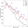 |
Fig. 1. Teff as a function of spectral type for solar-metallicity M dwarfs (black diamonds with line), sdMs (red dots), esdMs (green triangles), and usdMs (blue squares). Error bars on spectral types and model parameters are marked for sdMs only for clarity purposes. Error bars on spectral type and temperatures are ±0.25 and ±100 K, respectively. The point for the sdM7 subdwarf corresponds to LHS 377 from Rajpurohit et al. (2016). |
We note that the temperature scale of the line fitting option tends to infer lower effective temperatures by at least 100 K with a similar interval for temperatures hotter than 3400 K, producing ranges of 3700–2700 K. The agreement is better at lower temperatures and within the uncertainty of 100 K (Tables B.2 and B.4). We also find that the fit to the optical region only yields typically lower effective temperature by 100 K–200 K (Table B.5).
5.3. Gravity scale
Subdwarfs are old low-mass stars that belong to the thick disk or halo of our Galaxy. On average, they are much older than their solar-metallicity counterparts. Monteiro et al. (2006) identified several white dwarf–subdwarf systems in the thick disk and derived ages of 6–9 Gyr for two of them with M subdwarf companions. From the comparison with FGK stellar templates selected as benchmarks for the Gaia mission (Jofré et al. 2014), Scholz et al. (2015) inferred a possible age of 12 Gyr for an ancient metal-poor (−2.0 ± 0.2 dex) F-type star member of the Galactic halo due to its large tangential velocity. On average, we expect our sample to be older than 5 Gyr.
From the fit of the BT-Settl models to the full VIS+NIR SED of our M subdwarfs, we infer gravities of 4.5–5.5 dex for all metal classes, except for one object with log (g) = 6.0 dex (usdM3.0; see discussion section). However, we observe a possible trend of increasing mean gravity with lower metallicity, going from 5.0 dex for sdMs to 5.5 dex for esdMs and usdMs (Fig. 2). We note that the range of gravities of the CIFIST models is limited to 6.0 dex but higher gravities are desirable to corroborate this statement. We also note that the fit to the optical region only yields typically lower gravities by 0.5–1.0 dex (Table B.5).
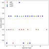 |
Fig. 2. Gravity as a function of spectral type for sdMs (red dots), esdMs (green triangles) and usdMs (blue squares). Error bars on spectral type and gravity are ±0.5 and ±0.5 dex, respectively. The point for the sdM7 subdwarf corresponds to LHS 377 from Rajpurohit et al. (2016). |
If we average the gravities for the metallicities derived from the model fit independently from the metal class (i.e. sdMs, esdMs, usdMs), we observe that targets with metallicities of −0.5 dex have on average lower gravities (∼4.9 dex) than more metal-poor objects where mean gravities lie between 5.2 and 5.3 dex. The difference in gravity between field M dwarfs and M subdwarfs is below our error bar of 0.5 dex, while the difference between metallicities is five times smaller than our error bars.
5.4. Metallicity scale
Our work extends the current metallicity scale of M dwarfs to metallicities below −0.5 dex with an accuracy on the calibration of the order of 0.25–0.5 dex. The classification is available in the optical for subdwarfs (Gizis 1997; Lépine et al. 2007; Jao et al. 2008; Savcheva et al. 2014; Kesseli et al. 2017) but this is the first time this has been attempted for a large sample of M0–M9 dwarfs (see also Rajpurohit et al. 2016). The determination of the metallicity scale of subdwarfs is key for several reasons. First, the range of metallicities for M subdwarfs is presently poorly constrained for these objects that represent the first generation of stars and are key sources to study the chemical evolution of our Galaxy. On the other hand, M dwarfs are becoming popular to search for low-mass planets by the radial velocity and transit techniques, leading independent groups to look at their metallicity. Nonetheless, all the studies referenced in the introduction focussed on M dwarfs with metallicity slightly below solar with calibrations accurate to < 0.15 dex either photometrically (Bonfils et al. 2005; Johnson & Apps 2009; Schlaufman & Laughlin 2010; Neves et al. 2012; Hejazi et al. 2015; Dittmann et al. 2016) or spectroscopically (Woolf & Wallerstein 2005, 2006; Bean et al. 2006; Woolf et al. 2009; Rojas-Ayala et al. 2010, 2012; Muirhead et al. 2012; Terrien et al. 2012; Önehag et al. 2012; Neves et al. 2013, 2014; Hejazi et al. 2015; Newton et al. 2015; Lindgren et al. 2016).
The number of M dwarf hosts below 0.5 M⊙ and with metallicities lower than −0.5 dex is extremely small (≤0.2%) compared to the 3396 confirmed planets7. Only three metal-poor M dwarfs have one or several planets: Kapteyn (sdM1.0; Fe/H = −0.86 dex; Anglada-Escudé et al. 2014; Robertson et al. 2015), GJ 667 (K3V+K5V; Fe/H = −0.55 dex; Feroz & Hobson 2014; Anglada-Escudé et al. 2013; Delfosse et al. 2013), and Kepler 1124 (Fe/H = −0.59 dex; Morton et al. 2016). Another four Kepler M stars with masses in the range 0.5–0.6 M⊙ and metallicities between −0.5 and −1.0 harbour planets.
We present VLT/X-shooter spectra at resolutions of 5400 and 3900 in the VIS and NIR arms, respectively. We estimate metallicities that rely on models and synthetic spectra whose steps are 0.5 dex, which we set as our error bars. Overall, we find that the overall SEDs of sdMs, esdMs, and usdMs are best reproduced by metallicities between solar and −1.0 dex, −1.0 and −2.0 dex, and −1.0 and −2.5 dex, respectively (Fig. 3). We note that a few sdMs have solar metallicities, including the sdM6.5 (1610−0040), a known astrometric binary (Koren et al. 2016) with a mix of spectral features typical of both L subdwarfs and solar-type M dwarfs (Lépine et al. 2003; Reiners & Basri 2006; Cushing & Vacca 2006). We also emphasise that the two coolest sdMs (sdM8 and sdM9.5) in our sample have on average lower metallicities than sdMs earlier than sdM7, suggesting saturation of the metallicity index (Lépine et al. 2007) used in the classification of subdwarf (Zhang et al. 2017). We conclude that there is a trend towards lower mean metallicity from sdMs (−0.5 ± 0.5 dex) to esdMs (−1.5 ± 0.5 dex), and usdMs (−2.0 ± 0.5 dex), consistent with the original definition of these three metal classes. However, we observe variations from one object to another, preventing us from assigning a given M/H for each metal class. We note that the metallicity scale of the line fitting option differs significantly from the fit of the SEDs, producing lower metallicities by at least 1.0 dex. (Tables B.2 and B.4). We find the same trend if we consider only the optical range (600–1000 nm) for our fitting procedure.
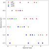 |
Fig. 3. Metallicity as a function of spectral type for sdMs (red dots), esdMs (green triangles) and usdMs (blue squares). Error bars on spectral type and metallicity are ±0.5 and ±0.5 dex, respectively. |
We compared our global results to the recent analysis of Rajpurohit et al. (2016) also based on VLT/X-shooter spectra but for a much smaller sample of subdwarfs: six sdMs (five sdM0.5–M3 and sdM7), two esdMs (esdM2 and esdM4), and usdM4.5. In their Table 2, they list two possible fits, which usually differ by either 100 K or 0.5 dex in gravity or metallicity. Our physical parameters agree with their results within 1–2σ of the steps of the synthetic SEDs (Table 2). The difference can be explained by the uncertainties on the spectral types, typically 0.5 sub-type. We conclude that both Teff-versus-spectral type relations are consistent within current error bars on observational and theoretical sides. Moreover, as stated in Rajpurohit et al. (2016), these results are fully consistent with the physical parameters derived from higher-resolution optical spectroscopy (Rajpurohit et al. 2014).
We can also compare our work to the physical parameters of the metal-poor binary G 224−58 AB composed of a esdK5 and a esdM5.5. Pavlenko et al. (2015) derived the temperature and gravity for the secondary (Teff = 3200 ± 100 K, log g = 5.0 ± 0.5), and inferred the metallicity from the primary ([Fe/H] = −1.92 dex). Their parameters are in good agreement with our values for the esdM5.5 (SDSS J09030795+0842432) in our sample: Teff = 3300 ± 100 K, log g = 5.5 ± 0.5 dex, and [Fe/H] = −1.5 ± 0.5 dex (Table 2). Their abundance analysis suggests that many elements (e.g. calcium; [Ca/H] = −1.39 ± 0.03) are over-abundant compared to iron. We do also find that, although the BT-Settl SEDs accurately reproduce the molecular bands of the observed spectra, they fail to fit the atomic lines of many elements like Fe, K, Na, and Ca. In other words, the atomic lines from the BT-Settl models are too broad and over-estimate the abundances of single elements (see Sect. 5.6). The disappearance of these elements in other molecules (e.g. CaOH) could also explain the observed discrepancy.
5.5. Masses
We inferred model-dependent masses for our sample of subdwarfs from their temperatures looking at the predictions of the NextGen models (Baraffe et al. 1997) and assuming ages of 10 Gyr for these old objects. Although this approach is not correct due to the different inputs physics in the NextGen and BT-Settl grids (computation available on France Allard’s webpage; Baraffe et al. 2015), it provides estimates on the masses of these low-metallicity M dwarfs. We derived masses below 0.35 M⊙ for the most massive M subdwarfs down to ∼0.087 M⊙ for the coolest objects in our sample, i.e. close to the stellar/substellar boundary with uncertainties of the order of 10% (Table 2). We note that the gravities quoted by the Baraffe et al. (1997) models are in the range log (g) = 5.0–5.5 dex, consistent with the aforementioned gravities derived from the synthetic SEDs within the error bars of 0.5 dex.
5.6. Abundances
We decided to work with the temperatures, gravities, and metallicities derived from the best fits to the optical regions only (Table B.5) to derive the abundances of several elements (Table 3). The relatively low resolution and reduced signal-to-noise ratios of the observed spectra limit the accuracy of our results. Moreover, we work here with metal-deficient stars, in which spectra are not critically affected by blending effects. We carried out the minimization procedure using the PHOENIX model atmospheres to compute synthetical spectra with the WITA program Pavlenko (1997). In these computations, we accounted for the main molecular opacity sources, as described in Pavlenko et al. (2015) and Pavlenko (2014). We employed the atomic line information from the VALD2 and VALD3 databases (Kupka et al. 1999; Ryabchikova et al. 2011). We selected a few spectral ranges with well-defined atomic lines and fitted them in the framework of the LTE approach to determine abundances of several elements listed in Table 3.
Spectral regions, elements, and their numbers of lines considered to derive abundances of our sample of subdwarfs.
To determine the abundances, we compared the residuals of the fluxes and reduced to the local continuum or pseudo-continuum of the observed spectra. We determined these continua/pseudo-continua for all spectral ranges given in Table 3. We carried out the computations for a 20-points abundance grid with a step 0.1 dex around the mean abundance for each metal and spectral subclass. The abundances correspond to over-abundances if they are positive, fixing the iron abundances to the metallicity derived from the model fit of the optical region, assuming a solar abundance of iron of −4.55 dex (Asplund et al. 2009).
When several lines are present in a given spectral range, we average the values of each abundance. We give the uncertainties on the abundances rounded to the nearest integer for a range of ±100 K in effective temperature, which represents the error on our model fits (and the step of the models). We note that the sodium, potassium, and neutral calcium lines are the most sensitive to small changes in effective temperature due to the low ionisation potentials. We estimate the formal accuracy of the abundance determination to be ±0.1 dex due to several uncertainties in the procedure, such as low signal-to-noise ratio and the determination of the levels of the continuum and pseudo-continuum. We list the final abundances of five elements (Na, K, Ca, Ti, and Fe) with their uncertainties in Table 4. Some of the stars, marked with an asterisk, have spectra with low signal-noise ratios, and therefore the abundances should be interpreted with caution.
Abundances for five elements (sodium, potassium, calcium, titanium, and iron) for each subtype and each metal class for a model atmosphere with a fixed temperature structure.
We should note that any significant changes in the abundance of alkali metals affect the fluxes of the continuum and hence, the strength of the lines. Alkali metals (Na, K, Ca, Mg) are known donors of free electrons in atmospheres of late-type stars. In our case, we re-computed the continuum fluxes for all the abundances, and so in a first approach we accounted for the effect of opacity changes. However, these changes of abundances may affect the temperature structure of the model atmosphere, changes not accounted for because we employed model atmospheres with a fixed temperature structure.
Our abundance analysis was performed for the model parameters obtained from the fits to observed SEDs (Sect. 4). Furthermore, the resolution of the fitted spectra was not high enough to get high-quality results. On the other hand, we work here with metal-deficient stars, in which spectra are not critically affected by blending effects. We determined a few spectral ranges with well defined atomic lines and fitted them in framework of the LTE approach. Despite all factors constraining the accuracy of our analysis we obtain several relatively robust results:
– We see a shift of Ti abundance distribution towards larger metallicities with respect to Fe for the lowest metallicities (top left panel of Fig. 4).
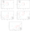 |
Fig. 4. Scatter in the abundances of sdMs (black symbols), esdMs (red), and usdMs (cyan) for several elements: Fe, Ti, K, Na, and Ca (Table 3). |
– We observe a Ca over-abundance in the atmospheres of all subdwarfs (top right panel of Fig. 4). This result agrees with the known enhancement of α elements in the atmospheres of halo dwarfs (e.g. Francois 1986; Nissen et al. 1994; Gratton & Sneden 1994; Fuhrmann et al. 1995).
– We find that K tends to be over-abundant at higher metallicities, that is the opposite effect to Na (middle panels of Fig. 4). This difference increases with lower metallicity and is most notable for usdMs. Perhaps these elements have different chemical histories. The difference is clearly seen in the comparison plot of the distribution of both species where the three metal classes are relatively well separated (bottom panel of Fig. 4).
– We cannot describe the abundances in the atmospheres of our targets with one parameter metallicity (Table 4 and Fig. 4).
6. Discussion
We observe that on average the optical range of the subdwarf spectra yields cooler temperatures, and lower gravities and metallicities. Hence, the availability of the NIR slope is quite important to determine the physical parameters of the three metal classes and break down the temperature-metallicity degeneracy present in the analysis of the sole visible range. The temperature sequence is well determined for all metal classes, with the earliest spectral types being the warmest cases. The metallicity is on average lower for the usdMs, with all three metal class being more metal poor than solar as expected. Those results are however global, with the physical parameters being sensitive to steps of the models in temperature, gravity, and metallicity. Smaller changes in those parameters are most likely limited by the quality (signal-to-noise ratio) and resolution of the X-shooter spectra.
We checked the few cases where our best fits suggest solar metallicity. There are four sdMs in this case (including the sdM6.5 specifically treated below) and only one esdM (esdM7.0) also discussed below. For the sdM1.5 we find that the best “FF” fits indicate solar metallicity while the other procedures suggest −0.5 dex. The inspection of the width of the lines (K, Na, Ca) is inconclusive, preventing a decision between one or the other metallicity (Fig. A.13). For the sdM3.0, all four fits are identical and suggest solar metallicity while the third best fit of the “FF” procedure yields −0.5 dex. The case of sdM5.0 indicates solar metallicity too but all other fits suggest −0.5 dex, confirmed by the width of the sodium and potassium lines, which advocate metallicity lower than solar with a temperature 3200 K. In the case of these three sdMs, we conclude that they might be peculiar somehow and require further investigation with better-quality data.
We also reviewed the four esdMs (esdM1.0, esdM1.5, esdM2.0, and esdM4.5) with differences of 200 K or more in temperature and ≥1.0 dex in metallicity comparing the four fitting procedures described in Sect. 5.1. We note that the three best fits of the “FF” procedure yield results within the step of the models. Therefore, we inspected the sodium, potassium, and calcium lines where we noticed that the best model fits occurred for the lowest metallicity values in all cases (Fig. A.14).
Finally, we observe four notable outliers discussed below after checking the best fits derived from the different procedures. We emphasise that we obtained one single spectrum per target.
– sdM0.0 is not included in our abundance analysis because the sodium and potassium lines are clearly resolved in our X-shooter spectrum. We confirm this target as a spectroscopic binary, which will be discussed in a separate paper. Any fit to spectral lines and abundance analysis on the spectrum taken at this specific epoch is therefore flawed.
– sdM6.5 (1610−0040) is a known astrometric binary (Koren et al. 2016) with a mix of spectral features typical of both L subdwarfs and solar-type M dwarfs (Lépine et al. 2003; Reiners & Basri 2006; Cushing & Vacca 2006). We derive a temperature of 2900 K with a gravity of 5.5 dex and solar metallicity with a reasonable “FF” model fit (Fig. A.1).
– esdM7.0 shows solar metallicity in the case of the full fitting procedure but lower metallicities with the other three cases. We inspected the sodium, potassium, and calcium lines of this object and conclude that the lines are broader than model predictions at solar metallicity, favouring the metal-poor solution. (Fig. A.14). We note that this object also has a low-quality spectrum.
– usdM3.0 exhibits a large difference when inspecting the best three chi-squared fits using the “FF” procedure, with variations of up to 200 K in temperature and 2.0 dex in metallicity. These differences are larger than any other object in our sample. We inspected the width and depth of the main sodium and potassium lines and find that they appear shallower with a potential double peak, which may indicate binarity (Fig. A.15). However, we obtained one single spectrum for this source so we cannot exclude other phenomenon like rotation, flare activity or spots that can affect our results. A few additional spectra with a minimum spectral resolution of 10000 are required to confirm this possibility, which would explain the large variations in the determination of the physical parameters.
7. Conclusions
Our atlas of VLT/X-shooter 0.45–2.5 μm moderate-resolution spectra represents an important database to classify metal-poor subdwarfs and represents an important resource for future large-scale surveys (WEAVE, 4MOST, LSST; Dalton et al. 2012, 2014; de Jong et al. 2014; Ivezic et al. 2008) and space missions such as the James Webb Space Telescope (Gardner et al. 2009) and Euclid (Mellier 2016). We derived radial velocities for all subdwarfs from the shift of the strongest optical lines. We inferred physical parameters (metallicities, temperatures, and gravities) for 43 metal-poor M dwarfs by comparing their SEDs over the 450–2500 nm range to the latest BT-Settl synthetic spectra. The main results of our analysis can be summarised as follows:
– The best gravity range for M subdwarfs is log (g) = 5.0–5.5 dex.
– The metallicities inferred from the BT-Settl models for sdMs, esdMs, and usdMs are −0.5, −1.5, and −2.0 dex with errors of 0.5 dex, respectively.
– The ranges in Teff for sdMs, esdMs, and usdMs are comparable and lie in the intervals 3700–2600 K, 3800–2900 K, and 3700–2900 K with uncertainties of 100 K, respectively.
– The Ca and Ti elements show an over-abundance while Na behaves in an opposite manner when compared to the iron abundance.
Improvements in the determination of the physical parameters and abundances of metal-poor low-mass dwarfs require refined, uniform, and complete model atmosphere grids to improve the fits. More advanced procedures are needed to improve the quality of the fits to observed SEDs treating atomic lines in a self-consistent way, with model atmospheres and spectra computed for one set of input parameters. Models should take into account the enhancement of C/O and improve the modelling of single lines updating abundances of the various elements present in cool atmospheres. To truly determine the physical parameters of M subdwarfs and test evolutionary models at low metallicity, the discovery of metal-poor low-mass transiting eclipsing binaries is key.
Last update on 10 October 2016 at exoplanetarchive.ipac.caltech.edu
Acknowledgments
NL was funded by the Ramón y Cajal fellowship number 08-303-01-02, and supported by the grants numbers AYA2010-19136 and AYA2015-69350-C3-2-P from Spanish Ministry of Economy and Competitiveness (MINECO). We thank Victor Béjar, and ZengHua Zhang for constructive comments on this work. The research leading to these results has received funding from the French Programme National de Physique Stellaire and the Programme National de Plan- etologie of CNRS (INSU). FA thanks financial support from the Fundación Jesús Serra for a two-month stay (Jan–Feb 2015) as a visiting professor at the Instituto de Astrofísica de Canarias (IAC) in Tenerife. This work is based on observations collected with X-shooter on the VLT at the European Southern Observatory, Chile, under programmes 089.C-0140(A), 091.C-0264(A), 092.D-0600(A), and 093.C-0610(A). This research has made use of the Simbad and Vizier databases, operated at the Centre de Données Astronomiques de Strasbourg (CDS), and of NASA’s Astrophysics Data System Bibliographic Services (ADS). Funding for the Sloan Digital Sky Survey IV has been provided by the Alfred P. Sloan Foundation, the U.S. Department of Energy Office of Science, and the Participating Institutions. SDSS-IV acknowledges support and resources from the Center for High-Performance Computing at the University of Utah. The SDSS web site is www.sdss.org. SDSS-IV is managed by the Astrophysical Research Consortium for the Participating Institutions of the SDSS Collaboration including the Brazilian Participation Group, the Carnegie Institution for Science, Carnegie Mellon University, the Chilean Participation Group, the French Participation Group, Harvard-Smithsonian Center for Astrophysics, Instituto de Astrofísica de Canarias, The Johns Hopkins University, Kavli Institute for the Physics and Mathematics of the Universe (IPMU)/University of Tokyo, Lawrence Berkeley National Laboratory, Leibniz Institut für Astrophysik Potsdam (AIP), Max-Planck-Institut für Astronomie (MPIA Heidelberg), Max-Planck-Institut für Astrophysik (MPA Garching), Max-Planck-Institut für Extraterrestrische Physik (MPE), National Astronomical Observatory of China, New Mexico State University, New York University, University of Notre Dame, Observatorio Nacional/MCTI, The Ohio State University, Pennsylvania State University, Shanghai Astronomical Observatory, United Kingdom Participation Group, Universidad Nacional Autónoma de México, University of Arizona, University of Colorado Boulder, University of Oxford, University of Portsmouth, University of Utah, University of Virginia, University of Washington, University of Wisconsin, Vanderbilt University, and Yale University.
References
- Adibekyan, V. Z., Sousa, S. G., Santos, N. C., et al. 2012, A&A, 545, A32 [NASA ADS] [CrossRef] [EDP Sciences] [Google Scholar]
- Allard, F., & Freytag, B. 2010, Highlights Astron., 15, 756 [NASA ADS] [Google Scholar]
- Allard, F., Baraffe, I., Chabrier, G., & Barman, T. 2003, ESA SP, 539, 247 [NASA ADS] [Google Scholar]
- Allard, F., Allard, N. F., Johnas, C. M. S., et al. 2007, IAU Symp., 240, 332 [NASA ADS] [Google Scholar]
- Allard, F., Homeier, D., & Freytag, B. 2012, Roy. Soc. London Philos. Trans. Ser. A, 370, 2765 [Google Scholar]
- Anglada-Escudé, G., Tuomi, M., Gerlach, E., et al. 2013, A&A, 556, A126 [NASA ADS] [CrossRef] [EDP Sciences] [Google Scholar]
- Anglada-Escudé, G., Arriagada, P., Tuomi, M., et al. 2014, MNRAS, 443, L89 [NASA ADS] [CrossRef] [Google Scholar]
- Asplund, M., Grevesse, N., Sauval, A. J., & Scott, P. 2009, ARA&A, 47, 481 [NASA ADS] [CrossRef] [Google Scholar]
- Baraffe, I., Chabrier, G., Allard, F., & Hauschildt, P. H. 1997, A&A, 327, 1054 [NASA ADS] [Google Scholar]
- Baraffe, I., Homeier, D., Allard, F., & Chabrier, G. 2015, A&A, 577, A42 [NASA ADS] [CrossRef] [EDP Sciences] [Google Scholar]
- Barber, R. J., Tennyson, J., Harris, G. J., & Tolchenov, R. N. 2006, MNRAS, 368, 1087 [NASA ADS] [CrossRef] [Google Scholar]
- Bean, J. L., Sneden, C., Hauschildt, P. H., Johns-Krull, C. M., & Benedict, G. F. 2006, ApJ, 652, 1604 [NASA ADS] [CrossRef] [Google Scholar]
- Bessell, M. S. 1991, AJ, 101, 662 [NASA ADS] [CrossRef] [Google Scholar]
- Bochanski, J. J., Hawley, S. L., Covey, K. R., et al. 2010, AJ, 139, 2679 [NASA ADS] [CrossRef] [Google Scholar]
- Bonfils, X., Delfosse, X., Udry, S., et al. 2005, A&A, 442, 635 [NASA ADS] [CrossRef] [EDP Sciences] [Google Scholar]
- Caffau, E., Ludwig, H.-G., Steffen, M., Freytag, B., & Bonifacio, P. 2011, Sol. Phys., 268, 255 [NASA ADS] [CrossRef] [Google Scholar]
- Cushing, M. C., & Vacca, W. D. 2006, AJ, 131, 1797 [NASA ADS] [CrossRef] [Google Scholar]
- Dalton, G., Trager, S. C., Abrams, D. C., et al. 2012, Proc. SPIE, 8446, 84460P [Google Scholar]
- Dalton, G., Trager, S., Abrams, D. C., et al. 2014, Proc. SPIE, 9147, 91470L [Google Scholar]
- de Bruijne, J. H. J. 2012, Astrophys. Space. Sci., 341, 31 [Google Scholar]
- de Jong, R. S., Barden, S., Bellido-Tirado, O., et al. 2014, Proc. SPIE, 9147, 91470M [CrossRef] [Google Scholar]
- Delfosse, X., Bonfils, X., Forveille, T., et al. 2013, A&A, 553, A8 [NASA ADS] [CrossRef] [EDP Sciences] [Google Scholar]
- Dittmann, J. A., Irwin, J. M., Charbonneau, D., & Newton, E. R. 2016, ApJ, 818, 153 [NASA ADS] [CrossRef] [Google Scholar]
- D’Odorico, S., Dekker, H., Mazzoleni, R., et al. 2006, Proc. SPIE, 6269 [Google Scholar]
- Feroz, F., & Hobson, M. P. 2014, MNRAS, 437, 3540 [NASA ADS] [CrossRef] [Google Scholar]
- Francois, P. 1986, A&A, 160, 264 [NASA ADS] [Google Scholar]
- Freytag, B., Steffen, M., Wedemeyer-Böhm, S., et al. 2010, Astrophysics Source Code Library [record ascl:1011.014] [Google Scholar]
- Fuhrmann, K., Axer, M., & Gehren, T. 1995, A&A, 301, 492 [NASA ADS] [Google Scholar]
- Gardner, J. P., Mather, J. C., Clampin, M., et al. 2009, Astrophys. Space Sci. Proc., 10, 1 [NASA ADS] [CrossRef] [Google Scholar]
- Gizis, J. E. 1997, AJ, 113, 806 [NASA ADS] [CrossRef] [Google Scholar]
- Gratton, R. G., & Sneden, C. 1994, A&A, 287, 927 [NASA ADS] [Google Scholar]
- Hejazi, N., De Robertis, M. M., & Dawson, P. C. 2015, AJ, 149, 140 [NASA ADS] [CrossRef] [Google Scholar]
- Henry, T. J., Jao, W.-C., Subasavage, J. P., et al. 2006, AJ, 132, 2360 [NASA ADS] [CrossRef] [Google Scholar]
- Ivezic, Z., Axelrod, T., Brandt, W. N., et al. 2008, Serb. Astron. J., 176, 1 [NASA ADS] [CrossRef] [Google Scholar]
- Jao, W.-C., Henry, T. J., Beaulieu, T. D., & Subasavage, J. P. 2008, AJ, 136, 840 [NASA ADS] [CrossRef] [Google Scholar]
- Jofré, P., Heiter, U., Soubiran, C., et al. 2014, A&A, 564, A133 [NASA ADS] [CrossRef] [EDP Sciences] [Google Scholar]
- Johnson, J. A., & Apps, K. 2009, ApJ, 699, 933 [NASA ADS] [CrossRef] [Google Scholar]
- Kausch, W., Noll, S., Smette, A., et al. 2015, A&A, 576, A78 [NASA ADS] [CrossRef] [EDP Sciences] [Google Scholar]
- Kesseli, A. Y., West, A. A., Veyette, M., et al. 2017, ApJS, 230, 16 [NASA ADS] [CrossRef] [Google Scholar]
- Kirkpatrick, J. D., Reid, I. N., Liebert, J., et al. 1999, ApJ, 519, 802 [NASA ADS] [CrossRef] [Google Scholar]
- Kirkpatrick, J. D., Gelino, C. R., Cushing, M. C., et al. 2012, ApJ, 753, 156 [NASA ADS] [CrossRef] [Google Scholar]
- Kirkpatrick, J. D., Schneider, A., Fajardo-Acosta, S., et al. 2014, ApJ, 783, 122 [NASA ADS] [CrossRef] [Google Scholar]
- Koren, S. C., Blake, C. H., Dahn, C. C., & Harris, H. C. 2016, AJ, 151, 57 [NASA ADS] [CrossRef] [Google Scholar]
- Kupka, F., Piskunov, N., Ryabchikova, T. A., Stempels, H. C., & Weiss, W. W. 1999, A&AS, 138, 119 [NASA ADS] [CrossRef] [EDP Sciences] [MathSciNet] [PubMed] [Google Scholar]
- Lépine, S., Rich, R. M., & Shara, M. M. 2003, ApJ, 591, L49 [NASA ADS] [CrossRef] [Google Scholar]
- Leggett, S. K., Allard, F., Berriman, G., Dahn, C. C., & Hauschildt, P. H. 1996, ApJS, 104, 117 [NASA ADS] [CrossRef] [EDP Sciences] [Google Scholar]
- Leggett, S. K., Allard, F., Dahn, C., et al. 2000, ApJ, 535, 965 [NASA ADS] [CrossRef] [Google Scholar]
- Lépine, S., Rich, R. M., & Shara, M. M. 2007, ApJ, 669, 1235 [NASA ADS] [CrossRef] [Google Scholar]
- Lindgren, S., Heiter, U., & Seifahrt, A. 2016, A&A, 586, A100 [NASA ADS] [CrossRef] [EDP Sciences] [Google Scholar]
- Lodieu, N., Espinoza Contreras, M., Zapatero Osorio, M. R., et al. 2017, A&A, 598, A92 [NASA ADS] [CrossRef] [EDP Sciences] [Google Scholar]
- Mellier, Y. 2016, COSPAR Meeting, Vol. 41, 41st COSPAR Scientific Assembly, Abstracts from the Meeting that was to be held 30 July – 7 August at the Istanbul Congress Center (ICC), Turkey, but was cancelled. See http://cospar2016.tubitak.gov.tr/en/, Abstract H0.2-1-16 [Google Scholar]
- Monteiro, H., Jao, W.-C., Henry, T., Subasavage, J., & Beaulieu, T. 2006, ApJ, 638, 446 [NASA ADS] [CrossRef] [Google Scholar]
- Morton, T. D., Bryson, S. T., Coughlin, J. L., et al. 2016, ApJ, 822, 86 [NASA ADS] [CrossRef] [Google Scholar]
- Muirhead, P. S., Hamren, K., Schlawin, E., et al. 2012, ApJ, 750, L37 [NASA ADS] [CrossRef] [Google Scholar]
- Neves, V., Bonfils, X., Santos, N. C., et al. 2012, A&A, 538, A25 [NASA ADS] [CrossRef] [EDP Sciences] [Google Scholar]
- Neves, V., Bonfils, X., Santos, N. C., et al. 2013, A&A, 551, A36 [NASA ADS] [CrossRef] [EDP Sciences] [Google Scholar]
- Neves, V., Bonfils, X., Santos, N. C., et al. 2014, A&A, 568, A121 [NASA ADS] [CrossRef] [EDP Sciences] [Google Scholar]
- Newton, E. R., Charbonneau, D., Irwin, J., & Mann, A. W. 2015, ApJ, 800, 85 [NASA ADS] [CrossRef] [Google Scholar]
- Nissen, P. E., Gustafsson, B., Edvardsson, B., & Gilmore, G. 1994, A&A, 285, 440 [NASA ADS] [Google Scholar]
- Nutzman, P., & Charbonneau, D. 2008, PASP, 120, 317 [NASA ADS] [CrossRef] [Google Scholar]
- Önehag, A., Heiter, U., Gustafsson, B., et al. 2012, A&A, 542, A33 [NASA ADS] [CrossRef] [EDP Sciences] [Google Scholar]
- Pavlenko, Y. V. 1997, Ap&SS, 253, 43 [NASA ADS] [CrossRef] [Google Scholar]
- Pavlenko, Y. V. 2014, Astron. Rep., 58, 825 [NASA ADS] [CrossRef] [Google Scholar]
- Pavlenko, Y. V., Zhang, Z. H., Gálvez-Ortiz, M. C., Kushniruk, I. O., & Jones, H. R. A. 2015, A&A, 582, A92 [NASA ADS] [CrossRef] [EDP Sciences] [Google Scholar]
- Plez, B. 1998, A&A, 337, 495 [NASA ADS] [Google Scholar]
- Plez, B. 2008, Phys. Scr. Vol. T, 133, 014003 [NASA ADS] [CrossRef] [Google Scholar]
- Quirrenbach, A., Amado, P. J., Seifert, W., et al. 2012, Proc. SPIE, 8446, 84460R [CrossRef] [Google Scholar]
- Rajpurohit, A. S., Reylé, C., Allard, F., et al. 2013, A&A, 556, A15 [NASA ADS] [CrossRef] [EDP Sciences] [Google Scholar]
- Rajpurohit, A. S., Reylé, C., Allard, F., et al. 2014, A&A, 564, A90 [NASA ADS] [CrossRef] [EDP Sciences] [Google Scholar]
- Rajpurohit, A. S., Reyle, C., Allard, F., et al. 2016, A&A, 596, A33 [NASA ADS] [CrossRef] [EDP Sciences] [Google Scholar]
- Reiners, A., & Basri, G. 2006, AJ, 131, 1806 [NASA ADS] [CrossRef] [Google Scholar]
- Robertson, P., Roy, A., & Mahadevan, S. 2015, ApJ, 805, L22 [NASA ADS] [CrossRef] [Google Scholar]
- Rojas-Ayala, B., Covey, K. R., Muirhead, P. S., & Lloyd, J. P. 2010, ApJ, 720, L113 [NASA ADS] [CrossRef] [Google Scholar]
- Rojas-Ayala, B., Covey, K. R., Muirhead, P. S., & Lloyd, J. P. 2012, ApJ, 748, 93 [NASA ADS] [CrossRef] [Google Scholar]
- Ryabchikova, T. A., Pakhomov, Y. V., & Piskunov, N. E. 2011, Kazan Izdatel Kazanskogo Universiteta, 153, 61 [NASA ADS] [Google Scholar]
- Savcheva, A. S., West, A. A., & Bochanski, J. J. 2014, ApJ, 794, 145 [NASA ADS] [CrossRef] [Google Scholar]
- Schlaufman, K. C., & Laughlin, G. 2010, A&A, 519, A105 [NASA ADS] [CrossRef] [EDP Sciences] [Google Scholar]
- Scholz, R.-D., Heber, U., Heuser, C., et al. 2015, A&A, 574, A96 [NASA ADS] [CrossRef] [EDP Sciences] [Google Scholar]
- Smette, A., Sana, H., Noll, S., et al. 2015, A&A, 576, A77 [NASA ADS] [CrossRef] [EDP Sciences] [Google Scholar]
- Sozzetti, A., Giacobbe, P., Lattanzi, M. G., et al. 2014, MNRAS, 437, 497 [NASA ADS] [CrossRef] [Google Scholar]
- Steiner, O., Vigeesh, G., Krieger, L., et al. 2007, Astron. Nachr., 328, 323 [NASA ADS] [CrossRef] [Google Scholar]
- Terrien, R. C., Mahadevan, S., Bender, C. F., et al. 2012, ApJ, 747, L38 [NASA ADS] [CrossRef] [Google Scholar]
- Testi, L. 2009, A&A, 503, 639 [NASA ADS] [CrossRef] [EDP Sciences] [Google Scholar]
- Tody, D. 1986, Proc. SPIE, 627, 733 [NASA ADS] [CrossRef] [Google Scholar]
- Tody, D. 1993, ASP Conf. Ser., 52, 173 [Google Scholar]
- Vernet, J., Dekker, H., D’Odorico, S., et al. 2011, A&A, 536, A105 [NASA ADS] [CrossRef] [EDP Sciences] [Google Scholar]
- Woolf, V. M., & Wallerstein, G. 2005, MNRAS, 356, 963 [NASA ADS] [CrossRef] [Google Scholar]
- Woolf, V. M., & Wallerstein, G. 2006, PASP, 118, 218 [NASA ADS] [CrossRef] [Google Scholar]
- Woolf, V. M., Lépine, S., & Wallerstein, G. 2009, PASP, 121, 117 [NASA ADS] [CrossRef] [Google Scholar]
- Zhang, Z. H., Pinfield, D. J., Gálvez-Ortiz, M. C., et al. 2017, MNRAS, 464, 3040 [NASA ADS] [CrossRef] [Google Scholar]
Appendix A: Model fit to VLT/X-shooter spectra
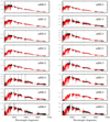 |
Fig. A.1. VLT/X-shooter UVB (450–550 nm), VIS (550–1000 nm) and NIR (1000–2500 nm) spectra of sdMs with spectral types from M0.0 to M9.5 (black lines) compared with the best BT-Settl spectra smoothed to the observed spectra. Spectral types are quoted in the top right corner for each subtype. The fits shown are for the FF case. |
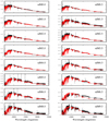 |
Fig. A.4. VLT/X-shooter UVB (450–550 nm), VIS (550–1000 nm) and NIR (1000–2500 nm) spectra of sdMs with spectral types from M0.0 to M9.5 (black lines) compared with the best BT-Settl spectra smoothed to the observed spectra. Spectral types are quoted in the top right corner for each subtype. The fits shown are for the LL case. |
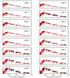 |
Fig. A.7. VLT/X-shooter UVB (450–550 nm), VIS (550–1000 nm) and NIR (1000–2500 nm) spectra of sdMs with spectral types from M0.0 to M9.5 (black lines) compared with the best BT-Settl spectra smoothed to the observed spectra. Spectral types are quoted in the top right corner for each subtype. The fits shown are for the FL case. |
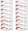 |
Fig. A.10. VLT/X-shooter UVB (450–550 nm), VIS (550–1000 nm) and NIR (1000–2500 nm) spectra of sdMs with spectral types from M0.0 to M9.5 (black lines) compared with the best BT-Settl spectra smoothed to the observed spectra. Spectral types are quoted in the top right corner for each subtype. The fits shown are for the LF case. |
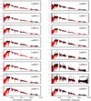 |
Fig. A.11. Same as Fig. A.10 for esdMs. |
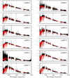 |
Fig. A.12. Same as Fig. A.10 for usdMs. |
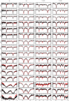 |
Fig. A.13. VLT/X-shooter UVB (450–550 nm), VIS (550–1000 nm) and NIR (1000–2500 nm) spectra of sdMs with spectral types from M0.0 to M9.5 (black lines) compared with the best BT-Settl spectra smoothed to the observed spectra for a few strong lines (sodium, potassium, and calcium). Spectral types are quoted in the top right corner for each subtype. |
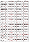 |
Fig. A.14. Same as Fig. A.13 for esdMs. |
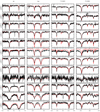 |
Fig. A.15. Same as Fig. A.13 for usdMs. |
Appendix B: Tables with physical parameters of subdwarfs
Derived physical parameters for sdMs, esdMs, and usdMs from the comparison between the observed X-shooter spectra and the BT-Settl synthetic spectra using the “FF” procedure.
Derived physical parameters for sdMs, esdMs, and usdMs from the comparison between the observed X-shooter spectra and the BT-Settl synthetic spectra using the “LL” procedure.
Derived physical parameters for sdMs, esdMs, and usdMs from the comparison between the observed X-shooter spectra and the BT-Settl synthetic spectra using the “FL” procedure.
Derived physical parameters for sdMs, esdMs, and usdMs from the comparison between the observed X-shooter spectra and the BT-Settl synthetic spectra using the “LF” procedure.
Derived physical parameters for sdMs, esdMs, and usdMs from the comparison between the optical region (600–1000 nm; “VV”) of the observed X-shooter spectra and the BT-Settl synthetic spectra.
All Tables
Adopted physical parameters for sdMs, esdMs, and usdMs from the comparison between the observed VLT/X-shooter spectra and the BT-Settl synthetic spectra from the fit of the overall SED.
Spectral regions, elements, and their numbers of lines considered to derive abundances of our sample of subdwarfs.
Abundances for five elements (sodium, potassium, calcium, titanium, and iron) for each subtype and each metal class for a model atmosphere with a fixed temperature structure.
Derived physical parameters for sdMs, esdMs, and usdMs from the comparison between the observed X-shooter spectra and the BT-Settl synthetic spectra using the “FF” procedure.
Derived physical parameters for sdMs, esdMs, and usdMs from the comparison between the observed X-shooter spectra and the BT-Settl synthetic spectra using the “LL” procedure.
Derived physical parameters for sdMs, esdMs, and usdMs from the comparison between the observed X-shooter spectra and the BT-Settl synthetic spectra using the “FL” procedure.
Derived physical parameters for sdMs, esdMs, and usdMs from the comparison between the observed X-shooter spectra and the BT-Settl synthetic spectra using the “LF” procedure.
Derived physical parameters for sdMs, esdMs, and usdMs from the comparison between the optical region (600–1000 nm; “VV”) of the observed X-shooter spectra and the BT-Settl synthetic spectra.
All Figures
|
Fig. 1. Teff as a function of spectral type for solar-metallicity M dwarfs (black diamonds with line), sdMs (red dots), esdMs (green triangles), and usdMs (blue squares). Error bars on spectral types and model parameters are marked for sdMs only for clarity purposes. Error bars on spectral type and temperatures are ±0.25 and ±100 K, respectively. The point for the sdM7 subdwarf corresponds to LHS 377 from Rajpurohit et al. (2016). |
| In the text | |
|
Fig. 2. Gravity as a function of spectral type for sdMs (red dots), esdMs (green triangles) and usdMs (blue squares). Error bars on spectral type and gravity are ±0.5 and ±0.5 dex, respectively. The point for the sdM7 subdwarf corresponds to LHS 377 from Rajpurohit et al. (2016). |
| In the text | |
|
Fig. 3. Metallicity as a function of spectral type for sdMs (red dots), esdMs (green triangles) and usdMs (blue squares). Error bars on spectral type and metallicity are ±0.5 and ±0.5 dex, respectively. |
| In the text | |
|
Fig. 4. Scatter in the abundances of sdMs (black symbols), esdMs (red), and usdMs (cyan) for several elements: Fe, Ti, K, Na, and Ca (Table 3). |
| In the text | |
|
Fig. A.1. VLT/X-shooter UVB (450–550 nm), VIS (550–1000 nm) and NIR (1000–2500 nm) spectra of sdMs with spectral types from M0.0 to M9.5 (black lines) compared with the best BT-Settl spectra smoothed to the observed spectra. Spectral types are quoted in the top right corner for each subtype. The fits shown are for the FF case. |
| In the text | |
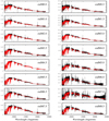 |
Fig. A.2. Same as Fig. A.1 for esdMs. |
| In the text | |
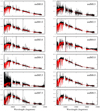 |
Fig. A.3. Same as Fig. A.1 for usdMs. |
| In the text | |
|
Fig. A.4. VLT/X-shooter UVB (450–550 nm), VIS (550–1000 nm) and NIR (1000–2500 nm) spectra of sdMs with spectral types from M0.0 to M9.5 (black lines) compared with the best BT-Settl spectra smoothed to the observed spectra. Spectral types are quoted in the top right corner for each subtype. The fits shown are for the LL case. |
| In the text | |
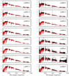 |
Fig. A.5. Same as Fig. A.4 for esdMs. |
| In the text | |
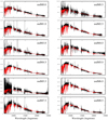 |
Fig. A.6. Same as Fig. A.4 for usdMs. |
| In the text | |
|
Fig. A.7. VLT/X-shooter UVB (450–550 nm), VIS (550–1000 nm) and NIR (1000–2500 nm) spectra of sdMs with spectral types from M0.0 to M9.5 (black lines) compared with the best BT-Settl spectra smoothed to the observed spectra. Spectral types are quoted in the top right corner for each subtype. The fits shown are for the FL case. |
| In the text | |
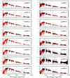 |
Fig. A.8. Same as Fig. A.7 for esdMs. |
| In the text | |
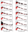 |
Fig. A.9. Same as Fig. A.7 for usdMs. |
| In the text | |
|
Fig. A.10. VLT/X-shooter UVB (450–550 nm), VIS (550–1000 nm) and NIR (1000–2500 nm) spectra of sdMs with spectral types from M0.0 to M9.5 (black lines) compared with the best BT-Settl spectra smoothed to the observed spectra. Spectral types are quoted in the top right corner for each subtype. The fits shown are for the LF case. |
| In the text | |
|
Fig. A.11. Same as Fig. A.10 for esdMs. |
| In the text | |
|
Fig. A.12. Same as Fig. A.10 for usdMs. |
| In the text | |
|
Fig. A.13. VLT/X-shooter UVB (450–550 nm), VIS (550–1000 nm) and NIR (1000–2500 nm) spectra of sdMs with spectral types from M0.0 to M9.5 (black lines) compared with the best BT-Settl spectra smoothed to the observed spectra for a few strong lines (sodium, potassium, and calcium). Spectral types are quoted in the top right corner for each subtype. |
| In the text | |
|
Fig. A.14. Same as Fig. A.13 for esdMs. |
| In the text | |
|
Fig. A.15. Same as Fig. A.13 for usdMs. |
| In the text | |
Current usage metrics show cumulative count of Article Views (full-text article views including HTML views, PDF and ePub downloads, according to the available data) and Abstracts Views on Vision4Press platform.
Data correspond to usage on the plateform after 2015. The current usage metrics is available 48-96 hours after online publication and is updated daily on week days.
Initial download of the metrics may take a while.