| Issue |
A&A
Volume 628, August 2019
|
|
|---|---|---|
| Article Number | A20 | |
| Number of page(s) | 13 | |
| Section | Interstellar and circumstellar matter | |
| DOI | https://doi.org/10.1051/0004-6361/201832632 | |
| Published online | 29 July 2019 | |
Cloudlet capture by transitional disk and FU Orionis stars
1
Zentrum für Astronomie, Heidelberg University,
Albert Ueberle Str. 2,
69120
Heidelberg,
Germany
e-mail: This email address is being protected from spambots. You need JavaScript enabled to view it.
2
Division of Particle and Astrophysical Science, Graduate School of Science, Nagoya University,
Furo-cho, Chikusa-ku,
Nagoya, Aichi
464-8602,
Japan
Received:
12
January
2018
Accepted:
22
June
2019
Abstract
After its formation, a young star spends some time traversing the molecular cloud complex in which it was born. It is therefore not unlikely that, well after the initial cloud collapse event which produced the star, it will encounter one or more low mass cloud fragments, which we call “cloudlets” to distinguish them from full-fledged molecular clouds. Some of this cloudlet material may accrete onto the star+disk system, while other material may fly by in a hyperbolic orbit. In contrast to the original cloud collapse event, this process will be a “cloudlet flyby” and/or “cloudlet capture” event: A Bondi–Hoyle–Lyttleton type accretion event, driven by the relative velocity between the star and the cloudlet. As we will show in this paper, if the cloudlet is small enough and has an impact parameter similar or less than GM*/v∞2 (with v∞ being the approach velocity), such a flyby and/or capture event would lead to arc-shaped or tail-shaped reflection nebulosity near the star. Those shapes of reflection nebulosity can be seen around several transitional disks and FU Orionis stars. Although the masses in the those arcs appears to be much less than the disk masses in these sources, we speculate that higher-mass cloudlet capture events may also happen occasionally. If so, they may lead to the tilting of the outer disk, because the newly infalling matter will have an angular momentum orientation entirely unrelated to that of the disk. This may be one possible explanation for the highly warped/tilted inner/outer disk geometries found in several transitional disks. We also speculate that such events, if massive enough, may lead to FU Orionis outbursts.
Key words: protoplanetary disks / stars: formation / ISM: clouds
© ESO 2019
1 Introduction
It is well known that stars rarely form in isolation. Star formation happens in giant molecular cloud complexes (GMCs), producing tens to many thousands of stars before the molecular cloud dissipates. The process is most likely primarily regulated by turbulence (Mac Low & Klessen 2004). The complex and chaotic process by which such turbulent cloud complexes produce stars can be modeled in quite some detail with 3D (magneto-)(radiation-)hydrodynamic simulations (e.g., Lee & Hennebelle 2016). Zoom-in simulations can follow this process from the lagest scales all the way down to the detailed dynamics and evolution of the protostellar/protoplanetary disk (e.g., Küffmeier et al. 2017). From such simulations it is known that the formation of a star in such an environment usually occurs in fits and starts rather than in a smooth single collapse, and that during these accretion events the angular momentum of the infalling material can change (Jappsen & Klessen 2004). In spite of these complexities, as a rule of thumb the formation of a star is usually regarded as a three-stage process: at first, a molecular cloud core becomes gravitationally unstable and starts to collapse, forming a protostar in the center (the class 0 stage). This protostar will initially be still surrounded by the infalling envelope material, which feeds the star and its protostellar disk (the class I stage). Once the collapse is over, the star and its protoplanetary disk are revealed (the class II stage). Such a simplification can be a powerful tool to understand the overall processes through which stars and their disks form and what properties they have (see e.g., Hueso & Guillot 2005; Dullemond et al. 2006). But it obviously also has its limitations.
For the computation of the Initial Mass Function from 3D star formation simulations it suffices to focus on the main infall phase, where most of the mass is accreted onto the star+disk system. Although the simple three-stage scenario mentioned above is too simplified, it is in general the case that most of the mass accretion is over by about one free-fall time scale. However, if we are interested in the protoplanetary disk and its evolution, even relatively low-mass (δM ≪ M⊙) accretion events occurring well after the main core collapse phase may become relevant, because these disks are thought to have masses of only 10−3 to at most ~10−1 M⊙. It is very natural to expect such late-time low-mass accretion events to take place, because after its formation, the “finished” star+disk system continues to travel through the remainder of the GMC. It may thus continue to accrete gas and dust from cloud fragments (henceforth called “cloudlets”) at a low rate through the Bondi–Hoyle–Lyttleton process (hereafter BHL process). Scicluna et al. (2014) argue that this might explain “late accretors”: stars that are relatively old (up to 30 Myr) but still show substantial accretion rates. Padoan et al. (2005) and Throop & Bally (2008) propose that the BHL process may be (in part) responsible for the observed  relation of pre-main-sequence stas (Muzerolle et al. 2003; Natta et al. 2004). Klessen & Hennebelle (2010) generalize this idea to a lower stellar velocity dispersion of ~0.2 km s−1, which they expect, instead of the canonical ~1 km s−1, and show that under those conditions even relatively high accretion rates can be obtained.
Since the interstellar medium in general and GMCs in particular have overall a fractal, clumpy structure, such late-time BHL accretion is presumably highly intermittent. Instead of encountering smooth large scale cloud structures, the star+disk system will likely encounter cloudlets of various densities and sizes. Cloudlets of sizes down to few hundreds (or even a few tens) of AU, and masses much less than a solar mass have been observed (Langer et al. 1995; Heiles 1997; Falgarone et al. 2004; Tachihara et al. 2012). These cloudlets are clearly stable against gravitational collapse and will not form stars themselves. Only through BHL accretion they may contribute to the mass of stars and their disks, if they pass too close by one of the young stars.
If the size of a cloudlet is of the same order as, or smaller than, the Hoyle–Lyttleton radius  (where v∞ is the relative velocity of the cloudlet with respect to the star), it becomes important to consider the precise impact parameter b at which the cloudlet approaches the star. A close enough approach of such a cloudlet to a star could lead to some of the matter remaining gravitationally bound to the star. We will henceforth call this process a “cloudlet capture event”. Statistically a perfect head-on “collision” (b = 0) is unlikely, while a very large impactparameter (b ≫ RHL) will not leadto any matter getting captured. Therefore cloudlet capture events will most commonly occur with impact parameters similar to the Hoyle–Lyttleton radius.
As a result, if the cloudlet (or part of it) is indeed captured by the star, it carries along a very high specific angular momentum with respect to the star. The captured material will thus not directly fall onto the star itself but will orbit around it. If the star does not have (or no longer has) a disk, then this leads to the formation of a new disk (or secondary disk). If a disk pre-exists, then the infalling matter will, in all likelihood, have a very different angular momentum axis than the disk. Depending on the mass ratio of the infalling cloudlet and the disk, this may tilt the pre-existing disk to another rotation axis. In fact, Thies et al. (2011) propose such a scenario to explain misaligned exoplanets. More recently, theexchange of disk material and angular momentum between two passing stars with disks has been studied as an alternative way of tilting the disk and the resulting planetary system produced by it (Xiang-Gruess & Kroupa 2017).
As a result of this angular momentum, cloudlet capture is thus a bit different from the usual BHL accretion: while BHL accretion is the accretion of matter directly onto the star, cloudlet capture, by virtue of the high angular momentum, typically leads to the formation (or replenishment) of a circumstellar disk. This material is bound to, but has not yet accreted onto the star. Angular momentum redistribution within the disk (either due to viscous disk accretion or gravitational instability) is then required to allow that mass to find its way to the stellar surface.
If a protoplanetary disk already exists before the cloudlet capture event sets in, then the infalling material interacts in a complicated way with the pre-existing disk. As already alluded to above, it can tilt the disk. But as has been shown by Lesur et al. (2015) and Hennebelle et al. (2017), such asymmetric infall can also drive spiral waves in the disk, which can transport angular momentum and cause inward motion of the gas. In their models, for the case of asymmetric infall (corresponding to the asymmetric cloudlet capture in our terminology), even an m = 2 mode is visible, which suggests a possible link to some of the observed m = 2 spirals seen in scattered light (e.g., Benisty et al. 2017, 2015) and at millimeter-wavelengths (e.g., Pérez et al. 2016; Huang et al. 2018). Furthermore, as shown by Bae et al. (2015), infall onto the disk can lead to the formation of vortices which, in addition to being potential sites of planet formation, also appear to have their observational counterparts (e.g., van der Marel et al. 2013; Casassus et al. 2012).
As we will show below, such off-center cloudlet capture events will often be accompanied by arc-shaped nebulosity, because the part of the cloudlet that is not accreted flies by in a hyperbolic orbit. Such “arcs” are, in fact, seen around several transitional disk stars and FU Orionis stars, as we will discuss in Sect. 4.
If the cloudlet is substantially larger than RHL, then it is still possible that the BHL accretion leads to a disk, as long as there is a sufficiently large density gradient in the cloudlet as the star passes through (Krumholz et al. 2005). For even larger cloudlets, however, the process would approach the classical BHL accretion (Krumholz et al. 2006).
We will show that for cases in which Rcloud ≫ b, instead of arcs, Bondi–Hoyle-like “tails” may be visible as reflection nebulosity. Such tails also appear to be seen, for instance in Z CMa (Liu et al. 2016) and SU Aurigae (Akiyama et al. 2019).
Since arc-shaped and tail-shaped reflection nebulosity appears to be found around several transitional disks and FU Orionis stars, it is tempting to speculate if the special properties of such sources may have their origin in cloudlet capture events in the not-too-distant past. Transitional disks are a special kind of protoplanetary disks which feature a large cavity in their inner regions. This often leads to a geometry featuring an inner-disk, a large gap and an outer disk. In some cases, the inner and outer disks appear to have wildly different rotation axes: for the stars HD 142527 and HD 100453 these are of order ~ 70° inclined with respect to each other (Marino et al. 2015; Benisty et al. 2017). In this paper we speculate whether the outer disks may have originated as a result of a cloudlet capture event. FU Orionis stars are stars that undergo a large accretion outburst. Given that several of these FU Orionis stars have arc/tail-shaped nebulosity nearby (e.g., Liu et al. 2016), we speculate that such outbursts may be triggered by a recent cloudlet capture event.
This paper is structured as follows: We will first make some analytic estimates in Sect. 2. In Sect. 3 we will show some results of simple hydrodynamic modeling. We will then discuss observations of reflection nebula patterns around a selected set of stars in Sect. 4. In Sect. 5 we will discuss the interpretation of these patterns in terms of the cloudlet capture and cloudlet flyby scenario, and whether there may be a link to transition disks and FU Orionis stars. We will also discuss the limitations of the model.
2 Estimations
Before we resort to numerical hydrodynamic calculations, we make a few simple estimations of the process of cloudlet capture and cloudlet flyby. For simplicity we assume the cloudlet to be spherical, with radius Rcloud, constant density ρcloud and temperature Tcloud, approaching the star with a velocity at infinity v∞ and impact parameter b. The cloudlet mass is much smaller than the stellar mass, and we assume that the cloudlet is in pressure equilibrium with a low-density warm neutral medium of Twnm = 8000 K (Field et al. 1969). The motion of the cloud, as it approaches the star, will thus initially be largely ballistic.
2.1 Critical impact parameter
A test particle approaching the star with impact parameter b and velocity v∞ will follow a hyperbolic orbit with a deflection angle of
 (1)
(1)
where the eccentricity e is defined as
 (2)
(2)
and the critical impact parameter bcrit is defined as
 (3)
(3)
The closest approach occurs at a distance  . The meaning of bcrit is the impact parameter for which the deflection angle is 90°. For b = bcrit the closest approach occurs at 0.41 bcrit. For a finite-size cloudlet we thus expect that an encounter with b ≃ bcrit will yield a well-defined arc, as the cloudlet will be tidally stretched roughly along the hyperbolic orbit. If the cloudlet has a radius Rcloud ≳ bcrit, some material from the cloudlet will get captured and forms a disk, while the rest of the cloudlet will fly by and forms the arc.
Given typical random velocities of filaments and young stars in giant molecular clouds of ~ 1 km s−1, and taking the typical stellar mass of a Herbig Ae star of M* = 2.5 M⊙, Eq. (3) with v∞ = 1 km s−1 yields bcrit ≃ 2200 au. This means that arc-shaped nebulosity around Herbig Ae stars, if observed, is expected to have spatialscales of the order of a few thousand au, and last a Kepler time scale of about 105 yr. According to Klessen & Hennebelle (2010), however, this estimate of v∞ = 1 km s−1 may be a bit on the high side. If we take instead v∞ = 0.5 km s−1 we obtain bcrit ≃ 104 au, and a time scale of half a million years.
2.2 Mass and size of cloudlets
Klessen & Hennebelle (2010) give a simple formula (their Eq. (19)) that relates the cloud/cloudlet mass to its size scale, based on observational data of GMCs from Falgarone et al. (2004). We rewrite that formula as:
 (4)
(4)
where we replaced the length scale L in Klessen & Hennebelle (2010) by 2 Rcloud. With a mean molecular weight of 2.3 for a gas consisting of molecular hydrogen and helium, this leads to a gas number density of
 (5)
(5)
There is, of course, some scatter in this relation, and it may vary somewhat between different GMCs. We will, however, use this relation for our model setup. Note that if we assume Rcloud ≃ bcrit, in which case we expect some of the cloudlet to be captured, and the other part to produce an strongly bent arc, then we find that  , which is a very steep dependency. Only a small variation in v∞ could lead to vastly different cloudlet masses under this assumption. For v∞ = 1 km s−1 we find Mcloud ≃ 1.5 × 10⁻³ M⊙, while for v∞ = 0.5 km s−1 we obtain Mcloud ≃ 3.5 × 10⁻² M⊙. Note that all these values assume a stellar mass of 2.5 M⊙, appropriate for a Herbig Ae star.
3 Hydrodynamic models
3.1 Numerical hydrodynamic model setup
Using the PLUTO hydrodynamics code1 (Mignone et al. 2007) we now demonstrate that the process of cloudlet capture is often associated with the formation of an arc-shaped reflection nebula like the ones seens around some transition disks and FU Orionis stars. We will focus on these large-scale features, and leave the detailed study of the formation and/or feeding of the disk to a follow-up paper (Küffmeier et al., in prep.).
For our model we choose the same simple scenario of a spherical cloudlet approaching the M* = 2.5 M⊙ star as in Sect. 2. Given the radius of the cloudlet Rcloud, the cloudlet gas density is given by Eq. (5). We place this cloudlet at the start of the simulation at a distance from the star substantially larger than bcrit (Eq. (3)), so that the initial movement of the cloudlet will be nearly linear. We set v∞ = 1 km s−1. The critical impact parameter is then bcrit = 2200 au.
We do two sets of models: adiabatic models and isothermal models, representing two extreme cases: that of no cooling and that of instant thermal adaption to the environment. We do not include time-dependent heating/cooling in the models. We also do not include magnetic fields, although they likely play a role.
For the adiabatic model we choose Tcloud = 30 K as the cloudlet temperature. The cloudlet must be embedded in a warm neutral medium in order to be kept under pressure, otherwise it will thermally expand well before it reaches the star. This warm neutral medium is set at a temperature of 8000 K. By demanding pressure equilibrium, the density of this medium is set. The ratio of specific heats is γ = 5∕3 for both the cold cloudlet (because molecular hydrogen is too cold to excite rotational levels) and for the warm neutral medium (because the hydrogen will be atomic). One problem with the adiabatic model assumption is that material that gets captured inside the potential well is likely to be shock-compressed and hot. This prevents the formation of a disk, and it will cause most of the captured material to “bounce back” and escape again in a wide range of directions. The isothermal models do not have this problem. A disk can be readily formed. But for the isothermal model it is impossible to embed the cloudlet into a confining medium (it would make the model non-isothermal). In principle one could make an initial condition consisting of two isothermal states: a cold isothermal cloudlet inside a hot isothermal medium, as we do for the adiabatic case. But some mixing between the two phases will occur due to numerical diffusion, at which point it will no longer be possible to decide which of the two temperatures to take. The cloudlet expansion problem can thus not be avoided for the isothermal models, and a cloudlet can therefore not really travel very far before it thermally expands again and dissipates. In a supersonically turbulent star formation environment such short-lived cloudlets can form through colliding flows. In fact, 3D simulations of turbulent molecular cloud complexes show that such transient cloudlets are formed (anddissipated) all the time (Mac Low & Klessen 2004). In our isothermal models we therefore put the cloudlet initially already much closer to the star than in the adiabatic models, and we set the temperature to Tcloud = 10 K. In this way thecloudlet can get captured before it dissipates.
The adiabatic models are set up in Cartesian coordinates, in a flattened box with x ∈ [−2L, L], y ∈ [−L, L] and z ∈ [−L∕4, L∕4], where L = 4.6 Rcloud is chosen such that the cloudlet fits vertically inside the box. The cloudlet is initially placed at x = − 1.7 L, y = −b and z = 0, or in vector form  . For the isothermal models the box size is x ∈ [−L, L], y ∈ [−L, L] and z ∈ [−L∕4, L∕4] and the initial position is at
  . The initial velocity of the gas is taken to be constant throughout the grid, with velocity vector v = (1, 0, 0) km s−1. The grid is composed of 384 × 256 × 64 grid cells for the adiabatic models and 256 × 256 × 64 grid cells for the isothermal models. The star is located at x = (0, 0, 0). Given the mirror symmetry in the z-plane, we only model the upper half, and put a mirror symmetry boundary condition at z = 0. The conditions at the other boundaries are simply copies of the warm neutral medium hydrodynamic state in the ghost cells. This allows waves to flow off the grid without much reflection. The gravitational potential is smoothed near the origin as
  , with smoothing radius rsm = 0.013 L. The model does not include self-gravity, nor a gravitational back-reaction onto the star. We run the model for 3 crossing times along the x-axis and make 61 dumps in equal time intervals. PLUTO works in dimensionless code units; we choose a length unit of 100 au, a velocity unit of 1 km s−1 and a density unit of 103 mp, with mp being the proton mass. But given the hydrodynamic nature of this model setup, the results are scalable.
The only remaining dimensionless physical free parameters of this setup are Rcloud∕bcrit and b∕bcrit.
Overview of the model parameters.
3.2 Postprocessing radiative transfer for scattered light images
The appearance of the cloudlet, as it flies by and/or partly gets captured, can be estimated using a simple radiative transfer setup. Rather than applying a fully-fledged Monte Carlo radiative transfer code such as RADMC-3D, we make use of the fact that these cloudlets are typically optically thin to stellar radiation. The scattering source function at each location x is then
 (6)
(6)
where  is the stellar flux as seen at x
 (7)
(7)
with r ≡|x| and  is the stellar luminosity at frequencyν. The dust density ρd(x) is taken to be 0.01 times the gas density ρg(x) and the dust scattering opacity
  is computedusing Mie theory for spherical dust grains with a Gaussian size distribution centered around a radius of a = 1 μm and a half-width in lg(a) of 0.05, made of pyroxene with 70% magnesium with a material density of 3 g cm−3. The function φ(θ) is the scattering phase function, where θ(x) is the angle between the stellar radiation at position x and the observer. We put the observer at z = +∞, so that
 (8)
(8)
with  . The phase function is normalized such that for isotropic scattering one would have φ(θ) = 1. We use the Henyey–Greenstein phase function with g computed with the Mie algorithm from ⟨cos(θ)⟩. After computing
  in each cell in the grid, we numerically integrate the formal radiative transfer equation from z = −∞ to z = + ∞ to obtain the scattered light image:
 (9)
(9)
where the contribution is only non-zero within the grid spanning between z = −L ∕ 4 and z = +L ∕ 4. We carry out this computation at a wavelength of λ = 0.65 μm. The stellar radius is taken to be R* = 2.4 R⊙ and the effective temperature of the star is T* = 104 K. For simplicity we assume a Planck spectrum, but one could also take e.g. a Kurucz spectrum. For our choice we obtain Lν = 1.96 × 10²⁰ erg s−1 Hz−1. The scattering opacity at this wavelength is  , which is cross section per gram of dust; we assume a dust-to-gas ratio of 0.01. The Henyey–Greenstein phase parameter at this wavelength is g = 0.73.
3.3 Results of the adiabatic models
The parameters of the adiabatic models A1, A2 and A3 are listed in Table 1. All models have approach-velocity v∞ = 1 km s−1, cloudlet temperatureTcloud = 30 K, and stellar mass M* = 2.5 M⊙.
In Fig. 1a time sequence of column density and synthetic scattered light images is shown for adiabatic model A1, which has Rcloud = 0.4 bcrit = 887 au and b = 0.8 bcrit = 1774 au.
This is a model in which the cloudlet impact parameter is small enough to cause a substantial gravitational deflection of the orbit of the cloudlet, but the cloudlet is itself too small to be partially captured by the star. It results in an curved flyby and a clear arc-shaped reflection nebula. The vast majority of the mass of the cloudlet flies by, but one can still notice a tiny bit of reflection much closer to the star, indicating that not all of the cloudlet mass avoided capture.
In Fig. 2 the same images are shown for adiabatic model A2, which has a larger cloudlet radius (Rcloud = 0.6 bcrit = 1330 au) but still the same impact parameter as in model A1. In this case the cloudlet is sufficiently large that a non-negligible amount of material is captured and remains bound, while the remainder of the cloudlet flies by. Hence, during the closest approach of the cloudlet, both an arc is seen as well as freshly captured circumstellar material. Still, most of the material avoids capture and escapes.
Finally in Fig. 3 a time sequence is shown for adiabatic model A3, which has Rcloud = 1.2 bcrit = 2662 au and b = 1.0 bcrit = 2218 au. In this case an arc is seen, but also a Bondi–Hoyle type tail superposed on it. This is because not all matter of the cloudlet passes by the star from one side. Some of the cloudlet material has, so to speak, a negative impact parameter, and collides with the majority of material coming from the positive impact parameter side. As in the case of model A2, some material remains bound to the star, forming a circumstellar disk.
In all these models the encounter of the cloudlet with the star leads to reflection nebulosity around the star of material that is mostly gravitationally unbound to the star. The arc shapes are the result of the gravitational deflection of the material that is passing by the star. The arc does not lie exactly along the hyperbolic orbit: due to the size of the cloudlet being of order bcrit, the arc, being initially stretched more or less along the orbit, eventually expands almost spherically away from the star.
Of the adiabatic models, the first one (A1) most clearly displays the arc-shaped nebulosity, and it behaves pretty much as one would expect on the basis of the ballistic arguments of Sect. 2. For A2, and even more so for A3, this simple picture fails,because the ballistic orbits cross each other, leading to the gas being shocked, and deflected from its ballistic path.
 |
Fig. 1 Snapshots of model A1 with Rcloud = 0.4 bcrit = 887 au and b = 0.8 bcrit = 1774 au. Left panel: column density, right panel: synthetic scattered light image at λ = 0.65 μm. In each panel, the 3 × 3 subpanels are different times, where time goes from top-left to bottom-right with intervals of 1934 yr. The yellow dot marks the location of the star. Note that the model domain extends well beyond the field of view shown here. |
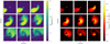 |
Fig. 2 As Fig. 1 but now for model A2 which has a larger cloudlet size. Note the different axis size compared to Fig. 1. |
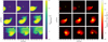 |
Fig. 3 As Fig. 1 but now for model A3 which has Rcloud = 1.2 bcrit = 2662 au and b = 1.0 bcrit = 2218 au. Note the different axis size compared to Fig. 1. |
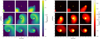 |
Fig. 4 As Fig. 1 but now for model I1 which has an isothermal equation of state. The parameters are with Rcloud = 0.4 bcrit = 887 au and b = 0.8 bcrit = 1774 au. Left panel: column density, right panel: synthetic scattered light image at λ = 0.65 μm. In each panel, the 3 × 3 subpanels are different times, where time goes from top-left to bottom-right with intervals of 1934 yr. The yellow dot marks the location of the star. |
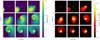 |
Fig. 5 As Fig. 4 but now for model I2, which has a larger cloudlet size (i.e. like model A2, but now isothermal). Note the different axis size compared to Fig. 4. |
3.4 Results of the isothermal models
Like for the adiabatic models the parameters are listed in Table 1. Models I1, I2 and I3 share the cloudlet radius and impact parameter with the models A1, A2, and A3, respectively. They can thus, to some extent, be regarded as their isothermal counterparts, albeit at lower temperature (Tcloud = 10 K instead of Tcloud = 30 K).
For model I1 the scattered light images are shown in Fig. 4. The arc structure is visible, in particular in the 6th time snapshot (middle row, right), but it is somewhat smeared out. This is due to the thermal expansion of the cloudlet during the capture. More prominent is the stretched “arm” seen in the third panel in the scattered light images (top row, right). This is the combined effect of tidal stetching of the accreting cloud and the 1 ∕ r2 dilution of the stellar light that scatters off the dust particles.
In Fig. 5 the results are shown of model I2 in which, compared to model I1 the cloudlet is larger. The differences with model I1 are not nearly as prominent as between models A2 and A1. The arc shaped structure is, however, weaker thanin model I1. In both models, however, the snapshots (the bottom row) show another prominent feature: an m = 1 spiralarm. This is most clearly seen in the column density maps, but it is also visible in the scattered light images.
Finally, in Fig. 6 the results of model I3 are shown. Compared to models I1 and I2 the spiral and arc features are less prominent, which is to be expected, since the ratio Rcloud ∕ bcloud is larger for this model, so that the role of the angular momentum of the cloudlet with respect to the star is less than in models I1 and I2. As aresult, the cloudlet-star interaction is more similar to classical Bondi–Hoyle accretion. Indeed, one can see a Bondi–Hoyle tail emerging in the top-right panel. This tail remains visible in the scattered light images, until the density drops too low.
In general one can see that for the isothermal models the arc-like shape of the nebulosity is less pronounced than for the adiabatic models. The reason is the thermal expansion of the cloudlet. For the isothermal models the cloudlet is not pressure-confined. It therefore expands as it approaches the star. As a result, the arc shaped reflection nebula is only relatively short-lived, as the cloudlet quite rapidly dissipates. In contrast, in the adiabatic model the cloudlet remains pressure-confined by the warm neutral medium. After passing by the star, the tidal stretching creates an arc. In the adiabatic case this arc remains geometrically narrow, while in the isothermal case the arc blows up and dissipates.
The thermal expansion of the isothermal models during the flyby also means that the dynamic behavior of the cloudlet is much less well described with ballistic trajectories. The analysis of Sect. 2 is therefore less applicable to the isothermal models as it is to the adiabatic models.
On the other hand, the isothermal models are more conducive to forming a disk. This has two reasons. One is that the cloudlet expands as it approaches the star, and thus more matter may get captured. Secondly, the captured material cannot get shock-heated, nor can mixing with the Warm Neutral Medium, and thus cannot build up sufficient pressure to counteract the formation ofa disk.
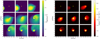 |
Fig. 6 As Fig. 4 but now for model I3 which has Rcloud = 1.2 bcrit = 2662 au and b = 1.0 bcrit = 2218 au (i.e. like model A3, but now isothermal). Note the different axis size compared to Fig. 4. |
3.5 Discussion of adiabatic versus isothermal results
The adiabatic models describe the case of a pressure-confined cloudlet passing by the star. They lead to arc-shaped and/or tail-shaped nebulosity around the star. But they are less efficient in capturing gas. The isothermal models, on the other hand, easily capture material from the cloudlet, and also produce Bondi–Hoyle like tails. But they are not efficient in forming arcs. Reality probably lies in between these two extreme cases. At large distances from the star the clouds may be pressure-confined by the warm neutral medium. But whether this is a long-lived state depends on the complexities of the phase transition between the cold and warm medium. However, once such a confined cloudlet gets tidally disrupted by the star, some of this cold cloud material gets compressed and may thereby start to cool more efficiently. This cooling will act against the adiabatic heating, and thus prevent the “bounce back” we see in the adiabatic models. If the cooling is fast enough, this material may stay cold during this compression, and can thus efficiently form a disk (or merge with an already existing disk). At the same time, if the cooling is not too fast, the pressure confinement of the tidally stretched flyby material may still keep the arc narrow. The exact outcome will depend on the intricacies of the heating/cooling physics.
If, on the other hand, cloudlets are not pressure confined, and instead they simply appear and disappear due to the supersonic turbulence in the molecular cloud complex, then the isothermal models may be not a bad description of the cloudlet capture process. Some of the material swings by the star, while the other part forms a disk. Arcs will then be rarer, but sometimes still visible. However, as the material approaches the star, the luminosity of the star itself will start to heat the material. The next step in the modeling would then be to include this effect. We will study this in a follow-up paper (Küffmeier et al., in prep.).
4 Observations
4.1 AB Aurigae (transition disk)
A promising candidate for such a “late stage asymmetric cloudlet capture” scenario is the star AB Aurigae. This star is among the brightest and nearest Herbig Ae stars with spectral type A0, an estimated mass of M* = 2.4 M⊙ (van den Ancker et al. 1998), (but see Hillenbrand et al. 1992, for another estimate of M* = 3.2 M⊙), an age estimate of between 2 Myr (van den Ancker et al. 1998) and 4 Myr (DeWarf et al. 2003), and a distance of 153 pc (Gaia DR1 data release: Gaia Collaboration 2016). It was classified as a “pre-transition disk” source by Honda et al. (2010), and as member of “group I” by Meeus et al. (2001). Optical imaging of AB Aurigae revealed not only the circumstellar disk at scales out to 450 AU, but also a large arc-shaped reflection nebula to the south-east at scales ranging from ~1300 AU out to ~6000 AU (Nakajima & Golimowski 1995; Grady et al. 1999) (see Fig. 7). The mass in the arc-shaped nebula was estimated by Nakajima & Golimowski (1995) to be at least 2 × 10⁻⁷M⊙, but perhaps more (an upper limit was not given). According to Semenov et al. (2005) there is evidence from DCO+ measurements with the IRAM 30 m telescope, as well as IRAS 60 μm measurements, of cold gas and dust material extending all the way out to 35 000 AU. The archival DSS images also show the reflection nebulosity in a shape of a streak extending along the east-west direction up to about 30 000 AU2. The disk itself, as seen in scattered light (Grady et al. 1999; Fukagawa et al. 2004), displays irregular spiral structures at scales of ~150–450 AU (see Fig. 7). At smaller scales the disk structure shows two roughly concentric rings in the H band, one with a radius of about 100 AU and an irregular ringlike/elliptic structure with a radius of about 35–60 AU (Oppenheimer et al. 2008; Hashimoto et al. 2011). The outer ring was also seen at 1.3 mm dust continuum (Piétu et al. 2005; Tang et al. 2012), albeit at a slightly larger radius of about 140 AU. These observations show this dust ring to be lopsided to the west, with an intensity contrast of about 3.
Resolved observations of the 12CO 2–1 line by Tang et al. (2012) give an intriguing, yet confusing picture of the dynamics of the system, which we reproduce in the text below for convenience. At large scales the 12CO 2–1 obtained with the IRAM 30 m telescope reveal only vague structures. But if these structures are real, then gas in the huge arc appears to show a radial velocity change along the arc from Δv ≃−0.57 km s−1 (to the east, compared to the systemic velocity) to Δv ≃ +0.85 km s−1 (to the south), which is substantial compared to the Kepler velocity at 1400 AU of vK (1400 AU) = 1.23 km s−1, but consistent with an elliptic or hyperbolic Keplerian orbit. Closer in, at the location of the spirals, the 12CO 2–1 data show two velocity components, one of which is also seen in 13CO 2–1 data byPiétu et al. (2005) and is believed to be from the disk, the other is not seen in the 13CO 2–1 data and is clearly from the spiral arms. The disk velocity component is consistent with a disk at an inclination of i = 23° (where i = 0° is face-on) and a position angle of the rotation axis of θ = −31.3° from north, assuming that the disk rotates counter-clockwise. However, the spiral component in the 12CO 2–1 data appears to behave exactly oppositely: if these data are interpreted as circular Keplerian rotation in the same direction on the sky as the disk component, one would obtain an inclination of i = − 20°. Alternatively one could interpret this as counter-rotating gas at an inclination of i = + 20°. At even smallerscales (insize of the 140 AU dust ring) gaseous spiral arms have been found by Tang et al. (2017). The origin of these spiral arms is not clear, but they may be induced by an unseen companion or planet.
Interpreting these data is not straightfoward, but there is little doubt that the disk of AB Aurigae is at this moment being fed with fresh material from its surroundings, as has been reported numerous times in the literature. The arc is, in our opinion, a stream of gas+dust stretched along its fly-by trajectory as a result of the tidal forces of AB Aurigae’s gravitational field. The free-fall time at the closest approach of 1300 AU is 3400 yr. With a conservative estimate of the velocity along this trajectory of 1 km s−1, the gas in the stream flows along its entire observable path in about 20 000 yr, which is less than 1% of the age of the star. The formation time scale of a star of this mass is of the order of 105 yr, meaning that any material that is directly related to the original cloud core must have already accreted or escaped the system long ago, by a factor of 20 or more in time. The material that is currently observed falling onto the disk (or flying by) is therefore unrelated to the original star formation event. It must be from a random cloud fragment of the larger scale molecular cloud complex. The extended CO as well as a reflection nebulosity in >10 000 AU scale support this picture.
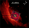 |
Fig. 7 Composite image of AB Aurigae. The large scale image is from Grady et al. (1999), taken with the Uni Hawaii 2.2 m Telescope at λ = 0.647 μm by P. Kalas. The medium scale inset is from the same paper, taken with the STIS instrument on the Hubble Space Telescope at λ = 0.57 μm. Both images were rotated with respect to their published form to put north up. The smallest inset is from Fukagawa et al. (2004), taking with the CIAO instrument on the Subaru telescope in the H band (λ ≃ 1.6 μm). The scale bar is 20′′ which for d = 153 pc (Gaia DR1 data release: Gaia Collaboration 2016) amounts to 3060 AU. The image shows the disk in the center out to at least 430 AU and a fainter much larger arc-shaped envelope with nearest approach to the star on the sky of about 1300 AU, but extending out to at least 6000 AU. All images used with permission of the authors of the referenced papers. |
4.2 HD 100546 (transition disk)
Hubble Space Telescope (HST) observations by Grady et al. (2001); Ardila et al. (2007) revealed that the Herbig Ae star HD 100546 is surrounded by a large disk with a radius of about 300 AU, as well as by tenuous envelope material out to about 1000 AU, in spite of its old age of 10 Myr (van den Ancker et al. 1998). The disk has m = 2 spiral structure globally (Grady et al. 2001; Ardila et al. 2007), albeit not nearly as strong as in sources such HD 100453 (Benisty et al. 2017). Quillen (2006) suggest that the spiral patterns can be explained by illumination from the star if the disk is warped. HD 100546 has also been known to feature an inner hole of about 13 AU radius (Bouwman et al. 2003; Grady et al. 2005), later confirmed in the direct imaging at optical and infrared wavelengths (Garufi et al. 2016; Follette et al. 2017), thus clearly making it a transition disk. It must also have at least some material close to the star (around 0.5 AU distance, where the dust sublimation radius is), owing to its observed near-infrared excess. Compared to AB Aurigae, however, the near-infrared excess of HD 100546 is much weaker. This suggests that the inner disk is substantially less dense in this source. Like in the case of AB Aurigae, the larger scale envelope material appears to be arranged in an arc-like shape around the south-west part of the disk at scales of up to 1000 AU, most clearly seen in Fig. 5 of the paper by Ardila et al. (2007), reproduced in Fig. 8.
Assuming that the spirals are trailing and are part of the disk itself, the disk rotates counter-clockwise on the sky. The fact that the CO 3–2 first moment map of (Walsh et al. 2014) shows a clear rotation profile with blueshifted emission on the south-east and redshifted emission on the north-west, means that the inclination of the rotation axis of the disk is pointing to the north-east, meaning that the near side of the disk is on the south-west. More precise analysis (Walsh et al. 2014) gives an inclination of i = 44 from pole-on, with the rotation axis of the disk pointing at a position angle on the sky of 56° counterclockwise from north. In the scattered-light image of Ardila et al. (2007) it appears that there is a dark lane on the near-side, which is consistent with the shape expected from an inclined disk with a bright scattered light surfaceon both the front and the back sides of the disk. If this interpretation is true, then this confirms the inclination and position angle inferred from the CO 3–2 data. The detailed look at the CO 3–2 first moment map provides a hint of a systematic deviation from the Keplerian velocity at the location of the south-west spiral at ~350 AU, though only by one velocity-resolution element (Δv ≃−0.21 km s−1). Inside 100 AU, non-Keplerian gas motion is suggested, which can be accounted for by the inner disk misaligned to the outer disk, or a radial flow of gas (Walsh et al. 2017).
The system therefore shows a similarity to AB Aurigae in its circumstellar structure, and looks like a more evolved counterpart of AB Aurigae. In particular, such a longevity of the large-scale envelope implies the star-forming environment rich in cloud fragments and a higher possibility of mass supply from the envelope onto the disk at later epochs than the original, main accretion phase of the protostar.
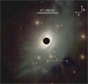 |
Fig. 8 Image of HD100546 from Ardila et al. (2007) (their Fig. 5) with RGB color coding according to R = B-band, G = V-band and B = I-band. The scale bar is 6′′ which for d = 109 pc (Gaia DR1 data release: Gaia Collaboration 2016) amounts to 654 AU. The image shows the disk in the center out to at least 300 AU, and a much fainter, much larger arc-shaped envelope out to 1000 AU going from south, via south-west to north-west (a dashed line was added to the image to indicate its position, as it is rather faint). Image used with permission of the authors of the referenced paper. |
4.3 Other transition disk sources
There are other transition disk sources with reflection nebulosity, though most are faint and do not show arc-like structures. In the case of HD 142527, a faint arc can perhaps be seen (see archival DSS images3) and a 500 AU-scale arm is found in CO observations (Christiaens et al. 2014), but it is certainly not massive enough to have a direct causal relationship with the tilted outer disk of HD 142527 (Marino et al. 2015). If the tilted disk around this star was caused by a cloudlet capture event, it must have taken place long enough ago, that no traces of this event are left. The star HD 97048 has quite some reflection nebulosity around it, and filamentary, spiral-like structures have been found at ~500 AU (Doering et al. 2007), but also here no clear arcs can be identified. RY Tau illuminates the surrounding nebula (Nakajima & Golimowski 1995), and the presence of an envelope has also been confirmed in the high resolution imaging of the inner 100 AU (Takami et al. 2013), but again the shape of the nebula cannot be recognized as an arc. Other transitional disks, for instance those listed in Table 1 of Espaillat et al. (2014) show no nebulosity based on the search using the DSS archival images, suggesting that the frequency of >1000 AU-scale nebulosity is ~10%. Note that the tenuous envelope of HD 100546 detected with HST cannot be identified in the DSS, and high-sensitivity observations for a statistically-meaningful sample are required to conclude the occurrence rate of such nebulosity. The probability of having a long-lived nebulosity seems to be lower for lower-mass stars than ~ 2 M⊙ since no T Tauri stars show reflection nebulae in the DSS search. However, for GM Aur (0.84 M⊙, Simon et al. 2000), the HST observations (Schneider et al. 2003) revealed the kinked, ribbon-like feature stretching toward northeast out to about 1700 AU from the star.
4.4 FU Orionis sources
FU Orionis stars are normally associated with reflection nebulosity unless they suffer from the large extinction by the parent molecular clouds. This is quite reasonable since most FU Orionis sources have prominent envelopes because of their youth, but it would be worth pointing out that at least two of them, FU Ori and Z CMa, are surrounded by the nebulae of 1000– 10 000 AU-scale in the shape of arcs (Nakajima & Golimowski 1995). When looking into their inner (<1000 AU) regions, the spatial structures are strikingly inhomogenious, which have been observed in scattered light in near-infrared (Liu et al. 2016). FU Ori shows an arm structure in the eastern side at 50–500 AU from the star, without a counter arm in the west. Z CMa also has an arm-like structure ~300 AU south of the star, in addition to a stream extending toward southwest. The companion stars are known for these stars, which complicates the interpretation of circumstellar structures, but in any case, such non-axisymmetry can be linked to the episodic accretion events of this class of objects. The other two FU Orionis sources in Liu et al. (2016) also show arms although the larger-scale envelopes do not look like arcs. Significant arc structures were found toward three stars out of 22 including “FUor-like” listed in Audard et al. (2014) in the DSS images: FU Ori, Z CMa and V646 Pup.
5 Discussion
5.1 Transitional disks caused by cloudlet capture?
Here we speculate whether cloudlet capture may be related to the class of large transitional disks, and might explain why some of them appear to be extremely warped. Transitional disks are protoplanetary disks with a large cavity. The gas and dust in this cavity has been removed, or at least strongly suppressed with respect to the outer disk. It is still a matter of debate which process has carved out this cavity. Many transition disks still have a small inner disk inside the cavity (e.g., Brown et al. 2007; Espaillat et al. 2010), and are sometimes called “pre-transition disks”. This leads to an “inner disk – gap – outer disk” geometry. The gap is, however, much more radially extended than one would expect for a gap carved out by a planet. A multi-planet system might open up a gap of that size, but it is hard to explain the depth of the gap with such a scenario (Zhu et al. 2011). A binary stellar companion may play a role. For instance, the star HD 142527, which features a prominent transition disk, has been resolved to consist of the main star and its M-dwarf companion at about 10 au projected distance (Biller et al. 2012), i.e. well within the 120 au gap of the disk. The inner disk appears to be resolved in recent images with SPHERE (Avenhaus et al. 2017), indicating a radius of a few au.
Recently it was found that in some transition disks the inner disk appears to be strongly tilted with respect to the outer disk (Marino et al. 2015). The striking two dark spots seen in scattered-light images of the outer disk of HD 142527 are naturally explained as being caused by the shadow cast by a heavily inclined (~ 70°) inner disk. The same phenomenon was observed in the disk of HD 100453 and also here the shadow cast by a heavily inclined (~ 72°) inner disk matches the observations (Benisty et al. 2017). This misalignment of the angular momentum vectors of the inner and outer disks in these two objects is so extreme (nearly perpendicular), that it is hard to imagine this to be caused by disk-interal processes or planetary objects.
In the case of HD 142527 the close-in binary companion may be orbiting out of the plane of the outer disk, which would explain why the inner disk is so strongly inclined. If the outer disk of this system is, however, of primordial nature, then this raises the question: why would the binary companion (which would be formed, one would think, from the same primordial disk) move on such a wildly out-of-plane orbit?
In the case of HD 100453 there appears to be a companion M star at 120 au projected distance, i.e. outside of the main star+disk system. Also this companion will likely have a strong dynamical influence on the disk, and may be responsible for the strong m = 2 spiral feature seen in this disk (Dong et al. 2016). If this companion orbits out of the plane of the disk, it might have caused the outer disk to precess and cause the misalignment of the inner and outer disk. But here again it is puzzling why the binary and the disk are so inclined with respect to each other.
One possible explanation was suggested by Owen & Lai (2017), who show that a binary companion inside the gap may lead the disk to undergo a secular precession resonance. This would make an initially in-plane binary+disk configuration to become mutually inclined.
Here we propose an alternative explanation: that these stars or binaries have, at some point after their formation, captured a low mass cloudlet from what is left of the surrounding clumpy giant molecular cloud (GMC) in which they were born. This cloudlet capture process replenishes the mass in the disk (or wraps an entirely new second generation disk around the system), but typically with an angular momentum axis different from that of the primordial disk. This is because the cloudlet originates from a different part of the GMC, and is thus dynamically unrelated to the original collapsing cloud core that produced the star and its primordial disk.
If at the time of the cloudlet capture event a small primordial disk still existed, the formation of the secondary disk would lead to the inclined inner/outer disk geometry. If the primordial disk is large, the captured cloudlet material would violently hydrodynamically interact with the primordial disk, possibly tilting its angular momentum axis. If the star is in fact a binary system (such as in HD 142527), then the circumbinary disk would likely be misaligned with the binary orbital plane. Any gas accretion from the circumbinary disk into the inner system would then likely get “reoriented” to the binary plane, again yielding an inclined inner/outer disk geometry.
A main caveat of this scenario is the required mass of the cloudlet that is captured, see Sect. 5.3. Also, in a process as complex as star formation in clusters it may not be possible to cleanly distinguish between what constitutes primordial infall and what is a late-stage cloudlet capture event, as we will discuss in Sect. 5.4.
5.2 Can cloudlet capture events trigger FU Orionis outbursts?
FU Orionis outbursts are relatively sudden, long-lasting outbursts of accretion activity in protostellar disk sources (Herbig 1977; Kenyon & Hartmann 1991). Many of these objects are heavily embedded in molecular clouds while some are more revealed objects. The outbursts are usually believed to be the result of an instability that periodically drives the disk from a long-lasting cold “low” state to a (relatively) short duration hot “high” state, and back again (e.g., Kenyon & Hartmann 1991; Armitage et al. 2001; Zhu et al. 2009, 2010). In the low state the disk cannot transport as much matter as it is being fed from outside (either from the outer disk of from an infalling envelope), and therefore starts to sequester this mass. Once the surface density of the disk reaches a critical value, the disk switches to the high state, rapidly flushes the sequestered mass onto the star, and returns to the low state. The low/high state are related to temperature through the ionization degree in the disk, as a lack of free ions and electrons leads to the formation of “dead zones” which are inefficient in driving accretion. The gravitational instability might play a role in triggering the transition from low to high. Vorobyov & Basu (2007, 2010) show that the interplay between continued feeding from the envelope causes the disk to display bursts of accretion driven by the gravitational instability, even if the turbulent viscosity of the disk is so low as to be unimportant.
The reflection nebulosity around several FU Orionis star systems (Liu et al. 2016) suggests that indeed FU Orionis outbursts could be related to an outside feeding of the disk. While this might be still part of the original star formation cloud collapse, these tail-like and arc-like features are suggestive of cloudlet capture events occurring. If this is the case, some FU Orionis objects may be “rejuvenated” disks.
We are, however, aware that this is very speculative. In particular, it would presumably require a relatively massive cloudlet capture event to take place. Such a cloudlet may even be optically thick and not show the kind of reflection nebula shapes discussed in this paper. It would be interesting, however, to further explore direct observational evidence of a link between infall onto the disk and the occurrance of FU Orionis outbursts.
EX Lupi (“EXOr”) outbursts are similar to FU Orionis outbursts, but they last much shorter. The star EX Lupi is the archetype of this class of objects and had its most recent outburst in 2008 lasting about half a year. These outburst are repetitive on time scales of tens of years. Given that this repetition rate is on a much shorter time scale than cloudlet capture events, it is unlikely that each EXOr outburst is associated with such an event. But like with FU Orionis outbursts, a single cloudlet capture event might lead to “overloading” of the disk, which leads to multiple outbursts on short time scales (D’Angelo & Spruit 2012).
5.3 Disk replenishment via cloudlet capture: the issue of cloudlet mass
In order for a late-type cloudlet capture event to significantly replenish the protoplanetary disk of a star, and thereby possibly tilt it to another rotation axis and/or trigger a FU Orionis activity, the mass of the cloudlet must be sufficiently large. Since often part of the cloudlet flies by and only a fraction of the cloudlet gets accreted, this mass would have to be accordingly larger to compensate for this inefficiency of capture.
In our models we rely on the mass-radius relation of cloudlets as given by Eq. (4). This relation from Klessen & Hennebelle (2010) was based on data from Falgarone et al. (2004) which go all the way down to scales of 5 × 10⁻³ pc and cloudlet masses of 10−4 M⊙. This relation has a scatter of about a factor of 102 in cloudlet mass at scales where the most data is available.
Arc-shaped features are expected to be most prominent for cloudlets that have radii similar to bcrit. For a star of 2.5 M⊙ and a relative velocity of v∞ = 1km s−1 this would be about 2200 au, which, according to the mass-radius relation, amounts to a mass of Mcloud ≃ 1.5 × 10⁻³ M⊙. The optical depth of the cloudlet at λ = 0.65 μm would be about 0.1.
This cloudlet mass is, however, on the low side for replenishing and old (or creating a new) disk around the star. For instance, the outer disk of the transition disk star HD 142527 was estimated by Casassus et al. (2012) to have a mass of about 0.1 M⊙. For AB Aurigae the disk mass estimated from dust continuum is between 0.01 and 0.04 M⊙ (Tang et al. 2012). For HD 100546 this is between 1 and 5 × 10⁻³ M⊙ (Dominik et al. 2003; Thi et al. 2011), although if we scale the estimated dust mass up with an assumed gas-to-dust ratio of 100 one would obtain a gas mass of 5 × 10⁻² M⊙ (Benisty et al. 2010; Thi et al. 2011).
Assuming instead a cloudlet mass of 0.1 M⊙, the mass-radius relation would yield a cloudlet radius of about 6 bcrit and an optical depth of 0.15. Such a largecloudlet would presumably not yield clearly identifiable arc-shaped reflection nebulosity, although it might generate Bondi–Hoyle tail-shaped features.
The mass-radius relation has, however, a spread in mass. If we would take an 0.1 M⊙ cloudlet of radius bcrit, a clear arc will be formed, but it will likely be optically thick. The cloudlet capture event would then look more like a class I object instead of a class II object.
5.4 Cloudlet capture versus the primordial collapse
In recent years numerous examples of misalignment in very young stellar objects have been found. For example, Lee et al. (2016) find misalignments between the outflow axes in binaries in the Perseus molecular cloud. Brinch et al. (2016) find a circumbinary disk around the class I binary star Oph IRS 43 that is misaligned with the orbit of the binary. Such findings show that star formation is not simple and that the angular momentum axis of infalling material varies with time, even already during the main cloud collapse phase. Numerical star formation modeling seems to confirm this (Bate et al. 2010; Bate 2018). It is therefore very well possible that the misalignment of the outer/inner disks of several transition disks could be directly inherited from the very early phases of the formation of the system. In the models of Bate (2018)this is most strikingly seen in his Fig. 2, where a binary star is formed with an outer disk misaligned by 75° with with the inner circumbinary disk. In that case, no late-stage cloudlet capture is necessary to create the strong misalignment, and the outer disk is then primordial, not secondary. But of course, a clear distinction between “primordial misalignment” and “misalignment due to late-stage cloudlet capture” may be hard to define since even the primordial accretion phase may be messy. Full zoom-in star formation simulations of the kind of Küffmeier et al. (2017) over a few million years may give the answer whether late stage cloudlet capture events can affect the protoplanetary disk’s axis. Such simulations will also show whether such secondary accretion events would produce larger disks than the primary events, because of large angular momentum resulting from the asymmetric approach of the cloudlet toward the star. This could be a criterion to distinguish the two.
5.5 Cloudlet capture in other contexts
The phenomenon of “cloudlet capture” also plays a role in the context of supermassive black holes in the center of galaxies, including our own. King & Pringle (2006) suggest that supermassive black holes may feed themselves through random infalling cloudlets with near-zero angular momentum. A somewhat larger angular momentum (i.e. impact parameter) would lead to the formation of an eccentric disk around the black hole and possibly the formation of stars in this disk (e.g. Bonnell & Rice 2008; Goicovic et al. 2016). In case of a binary black hole system the randomly oriented circumbinary disk that is formed in such an event (Dunhill et al. 2014) might play a role in reducing the orbital separation of the black holes and thus resolving the “last parsec problem” of supermassive black hole merging.
While qualitatively the two scenarios are similar, the main difference lies in the ratio of the gas temperature to the virial temperature. At the scale of r = 0.1 bcrit around a T Tauri or Herbig Ae star the virial temperature Tvir = μmpGM*∕kBr is of the order of 3000 K. If the gas has a temperature of 30 K, for instance, this leads to a disk vertical scale height of hp ∕r = cs∕ΩKr = ≃ 0.1 (where cs is the isothermal sound speed and ΩK the Kepler frequency). For molecular disks around supermassive black holes the ratio of the gas temperature to the virial temperature is orders of magnitude smaller due to the enormous depth of the gravitational potential well. The disks that are formed are therefore also geometrically much thinner, with values of the order of hp ∕r ≃ 10−3−10−2. The difference between the two cases is qualitatively the strongest during the approach of the cloudlet to the star/black hole: the gas temperatureplays a much larger role in the case of a cloudlet approaching the star, while in the case of clouds accreting onto a supermassive black hole the approach is more ballistic.
5.6 Scalability of the model
Because in our hydrodynamic model we have used simple equations of state (only adiabatic and isothermal, no cooling), the results of the calculations can be relatively easily scaled to other stellar masses, luminosities and cloudlet masses and sizes. Also the mass-size relation (Eq. (4)) does hot have to be strictly adhered to. The only non-scalable (dimensionless) parameters are b∕bcrit, Rcloud∕bcrit and the Mach number  . And of course the initial position of the cloudlet relatively close to the star for the isothermal models, in units of bcrit. The Mach number is likely to play only a limited role in the adiabatic models, given that the cloudlet is pressure confined by the warm neutral medium.
5.7 Caveats and future work
The simple modeling setup with a fixed grid that is used in this paper is not suited for studying the actual formation of a secondary disk and/or the cloud-disk interaction. Adaptive mesh refinement is unavoidable to get sufficient spatial resolution to resolve the vertical scale of the protoplanetary disk. Also a more realistic equation of state will be required to make quantitative conclusions. In a follow-up paper (Küffmeier et al., in prep.) we will present the results of cloudlet capture models simulated with the AREPO moving mesh code, in which we study, among other things, the properties of the resulting secondary disks, and the effects of more realistic equations of state. Further down the road it will be necessary to replace the simple initial conditions with a realistic environment: Starting with a large scale star formation model, and performing zoom-in simulations on individual stars, and modeling these well beyond their initial collapse phase.
Magnetic field may play a critical role as well. It is likely that low mass cloudlets are more magnetized (i.e. have a higher magnetic over gas pressure ratio) than the much more massive star-forming cloud cores. It is unclear how this may change the results of cloudlet capture. Magnetic pressure may give the cloudlet an “adiabatic-like” behavior, which would suppress capture of the gas, while magnetic tension may, on the contrary, extract angular momentum from the captured material, enhancing the capture of gas. And whether arc-shaped or tail-shaped features will be formed by the non-captured material, when magnetic fields are involved, is entirely unclear. On the other hand, it is known that filamentary structures spontaneously form when magnetic fields start to dominate over gas pressure. An extreme example of this are the coronal loops in the solar chromosphere and corona. But similar effects also occur in molecular cloud complexes (Hennebelle 2013). Clearly, MHD modeling will be needed to answer these questions.
6 Conclusions
Cloudlet capture is a process that can replenish the circumstellar environment of young stars even at a relatively late time after formation, as long as the star is still travelling within the star formation region and the material of the giant molecular cloud complex has not yet fully dissipated. As opposed to the “classical” Bondi–Hoyle–Lyttleton accretion, cloudlet capture involves cloudlets or cloud filaments that are of similar size as, or smaller than, the critical impact parameter  , with v∞ being the approach velocity. In such a case, the cloudlet brings a lot of angular momentum into the process. If the cloudlet passes by close enough to the star (with impact parameter similar to, or smaller than bcrit) this can lead to the capture of part of this cloudlet followed by the formation of a secondary disk or the replenishment of an already existing disk. The other part of the cloudlet will pass by in an arc. Some of this material may, in fact, still accrete if parts of the arc are elliptic instead of hyperbolic. Searching for such signatures around young stars may teach us about the frequency of such events, which gives constraints on the process of star formation and may help explain some of the more exotic protoplanetary disk sources such as tilted transition disks and FU Orionis outbursting stars.
Acknowledgements
We would like to thank Leonardo Testi, Hauyu Baobab Liu, Jonathan Williams, Peter Abraham, Agnes Kospal, Klaus Pontoppidan, Giovanni Rosotti, Thomas Haworth, Colin McNally, Willy Kley, Antonella Natta, Nienke van der Marel, Ewine van Dishoeck, Ralf Klessen, Philipp Girichidis, Patrick Hennebelle, Mario van den Ancker, Monika Petr-Gotzens, Adriana Pohl, Carsten Dominik, for useful discussions, and Daniel Thun for help with the Binac Cluster. The authors acknowledgesupport by the High Performance and Cloud Computing Group at the Zentrum für Datenverarbeitung of the University of Tübingen, the state of Baden-Württemberg through bwHPC and the German Research Foundation (DFG) through grant no INST 37/935-1 FUGG. This research was supported by the Munich Institute for Astro- and Particle Physics (MIAPP) of the DFG cluster of excellence “Origin and Structure of the Universe”, in particular the MIAPP workshop “Protoplanetary Disks and Planet Formation” in June 2017 where many of the above discussions took place which considerably helped to improve the argumentation. Part of this work was also funded by the DFG Forschergruppe FOR 2634 “Planet Formation Witnesses and Probes: Transition Disks” under grant DU 414/23-1. F.G. acknowledges support from DFG Schwerpunktprogramm SPP 1992 “Diversity of Extrasolar Planets” grant DU 414/21-1. The research of M.K. is supported by a research grant of the Independent Research Foundation Denmark (IRFD) (international postdoctoral fellow, project number: 8028-00025B). The hydrodynamics models were done with the PLUTO code (http://plutocode.ph.unito.it). Some supporting models (not shown in this paper) were performed with the AREPO code (https://wwwmpa.mpa-garching.mpg.de/~volker/arepo/). Finally, we would like to thank the anonymous referee for his/her patience and useful suggestions to improve the paper.
References
- Akiyama, E., Vorobyov, E. I., baobabu Liu, H., et al. 2019, AJ, 157, 165 [NASA ADS] [CrossRef] [Google Scholar]
- Ardila, D. R., Golimowski, D. A., Krist, J. E., et al. 2007, ApJ, 665, 512 [NASA ADS] [CrossRef] [Google Scholar]
- Armitage, P. J., Livio, M., & Pringle, J. E. 2001, MNRAS, 324, 705 [NASA ADS] [CrossRef] [Google Scholar]
- Audard, M., Ábrahám, P., Dunham, M. M., et al. 2014, Protostars and Planets VI (Tucson: University of Arizona Press), 387 [Google Scholar]
- Avenhaus, H., Quanz, S. P., Schmid, H. M., et al. 2017, AJ, 154, 33 [NASA ADS] [CrossRef] [Google Scholar]
- Bae, J., Hartmann, L., & Zhu, Z. 2015, ApJ, 805, 15 [NASA ADS] [CrossRef] [Google Scholar]
- Bate, M. R. 2018, MNRAS, 475, 5618 [NASA ADS] [CrossRef] [Google Scholar]
- Bate, M. R., Lodato, G., & Pringle, J. E. 2010, MNRAS, 401, 1505 [NASA ADS] [CrossRef] [Google Scholar]
- Benisty, M., Tatulli, E., Ménard, F., & Swain, M. R. 2010, A&A, 511, A75 [NASA ADS] [CrossRef] [EDP Sciences] [Google Scholar]
- Benisty, M., Juhász, A., Boccaletti, A., et al. 2015, A&A, 578, L6 [NASA ADS] [CrossRef] [EDP Sciences] [Google Scholar]
- Benisty, M., Stolker, T., Pohl, A., et al. 2017, A&A, 597, A42 [NASA ADS] [CrossRef] [EDP Sciences] [Google Scholar]
- Biller, B., Lacour, S., Juhász, A., et al. 2012, ApJ, 753, L38 [NASA ADS] [CrossRef] [Google Scholar]
- Bonnell, I. A., & Rice, W. K. M. 2008, Science, 321, 1060 [NASA ADS] [CrossRef] [PubMed] [Google Scholar]
- Bouwman, J., de Koter, A., Dominik, C., & Waters, L. B. F. M. 2003, A&A, 401, 577 [NASA ADS] [CrossRef] [EDP Sciences] [Google Scholar]
- Brinch, C., Jørgensen, J. K., Hogerheijde, M. R., Nelson, R. P., & Gressel, O. 2016, ApJ, 830, L16 [NASA ADS] [CrossRef] [Google Scholar]
- Brown, J. M., Blake, G. A., Dullemond, C. P., et al. 2007, ApJ, 664, L107 [NASA ADS] [CrossRef] [Google Scholar]
- Casassus, S., Perez M., S., Jordán, A., et al. 2012, ApJ, 754, L31 [NASA ADS] [CrossRef] [Google Scholar]
- Christiaens, V., Casassus, S., Perez, S., van der Plas, G., & Ménard, F. 2014, ApJ, 785, L12 [Google Scholar]
- D’Angelo, C. R., & Spruit, H. C. 2012, MNRAS, 420, 416 [NASA ADS] [CrossRef] [Google Scholar]
- DeWarf, L. E., Sepinsky, J. F., Guinan, E. F., Ribas, I., & Nadalin, I. 2003, ApJ, 590, 357 [NASA ADS] [CrossRef] [EDP Sciences] [Google Scholar]
- Doering, R. L., Meixner, M., Holfeltz, S. T., et al. 2007, AJ, 133, 2122 [NASA ADS] [CrossRef] [Google Scholar]
- Dominik, C., Dullemond, C. P., Waters, L. B. F. M., & Walch, S. 2003, A&A, 398, 607 [NASA ADS] [CrossRef] [EDP Sciences] [Google Scholar]
- Dong, R., Zhu, Z., Fung, J., et al. 2016, ApJ, 816, L12 [NASA ADS] [CrossRef] [Google Scholar]
- Dullemond, C. P., Natta, A., & Testi, L. 2006, ApJ, 645, L69 [NASA ADS] [CrossRef] [Google Scholar]
- Dunhill, A. C., Alexander, R. D., Nixon, C. J., & King, A. R. 2014, MNRAS, 445, 2285 [NASA ADS] [CrossRef] [Google Scholar]
- Espaillat, C., D’Alessio, P., Hernández, J., et al. 2010, ApJ, 717, 441 [NASA ADS] [CrossRef] [Google Scholar]
- Espaillat, C., Muzerolle, J., Najita, J., et al. 2014, Protostars and Planets VI (Tucson: University of Arizona Press), 497 [Google Scholar]
- Falgarone, E., Hily-Blant, P., & Levrier, F. 2004, A&SS, 292, 89 [Google Scholar]
- Field, G. B., Goldsmith, D. W., & Habing, H. J. 1969, ApJ, 155, L149 [NASA ADS] [CrossRef] [Google Scholar]
- Follette, K. B., Rameau, J., Dong, R., et al. 2017, AJ, 153, 264 [NASA ADS] [CrossRef] [Google Scholar]
- Fukagawa, M., Hayashi, M., Tamura, M., et al. 2004, ApJ, 605, L53 [NASA ADS] [CrossRef] [Google Scholar]
- Gaia Collaboration (Brown, A. G. A., et al.) 2016, A&A, 595, A2 [NASA ADS] [CrossRef] [EDP Sciences] [Google Scholar]
- Garufi, A., Quanz, S. P., Schmid, H. M., et al. 2016, A&A, 588, A8 [NASA ADS] [CrossRef] [EDP Sciences] [Google Scholar]
- Goicovic, F. G., Cuadra, J., Sesana, A., et al. 2016, MNRAS, 455, 1989 [NASA ADS] [CrossRef] [Google Scholar]
- Grady, C. A., Woodgate, B., Bruhweiler, F. C., et al. 1999, ApJ, 523, L151 [NASA ADS] [CrossRef] [Google Scholar]
- Grady, C. A., Polomski, E. F., Henning, T., et al. 2001, AJ, 122, 3396 [NASA ADS] [CrossRef] [Google Scholar]
- Grady, C. A., Woodgate, B., Heap, S. R., et al. 2005, ApJ, 620, 470 [Google Scholar]
- Hashimoto, J., Tamura, M., Muto, T., et al. 2011, ApJ, 729, L17 [NASA ADS] [CrossRef] [Google Scholar]
- Heiles, C. 1997, ApJ, 481, 193 [NASA ADS] [CrossRef] [Google Scholar]
- Hennebelle, P. 2013, A&A, 556, A153 [NASA ADS] [CrossRef] [EDP Sciences] [Google Scholar]
- Hennebelle, P., Lesur, G., & Fromang, S. 2017, A&A, 599, A86 [NASA ADS] [CrossRef] [EDP Sciences] [Google Scholar]
- Herbig, G. H. 1977, ApJ, 217, 693 [NASA ADS] [CrossRef] [Google Scholar]
- Hillenbrand, L. A., Strom, S. E., Vrba, F. J., & Keene, J. 1992, ApJ, 397, 613 [NASA ADS] [CrossRef] [Google Scholar]
- Honda, M., Inoue, A. K., Okamoto, Y. K., et al. 2010, ApJ, 718, L199 [NASA ADS] [CrossRef] [Google Scholar]
- Huang, J., Andrews, S. M., Pérez, L. M., et al. 2018, ApJ, 869, L43 [NASA ADS] [CrossRef] [Google Scholar]
- Hueso, R., & Guillot, T. 2005, A&A, 442, 703 [NASA ADS] [CrossRef] [EDP Sciences] [Google Scholar]
- Jappsen, A.-K., & Klessen, R. S. 2004, A&A, 423, 1 [NASA ADS] [CrossRef] [EDP Sciences] [Google Scholar]
- Kenyon, S. J., & Hartmann, L. W. 1991, ApJ, 383, 664 [NASA ADS] [CrossRef] [Google Scholar]
- King, A. R., & Pringle, J. E. 2006, MNRAS, 373, L90 [NASA ADS] [CrossRef] [Google Scholar]
- Klessen, R. S., & Hennebelle, P. 2010, A&A, 520, A17 [NASA ADS] [CrossRef] [EDP Sciences] [Google Scholar]
- Krumholz, M. R., McKee, C. F., & Klein, R. I. 2005, ApJ, 618, 757 [NASA ADS] [CrossRef] [Google Scholar]
- Krumholz, M. R., McKee, C. F., & Klein, R. I. 2006, ApJ, 638, 369 [NASA ADS] [CrossRef] [Google Scholar]
- Küffmeier, M., Haugbølle, T., & Nordlund, Å. 2017, ApJ, 846, 7 [NASA ADS] [CrossRef] [Google Scholar]
- Langer, W. D., Velusamy, T., Kuiper, T. B. H., et al. 1995, ApJ, 453, 293 [NASA ADS] [CrossRef] [Google Scholar]
- Lee, Y.-N., & Hennebelle, P. 2016, A&A, 591, A30 [NASA ADS] [CrossRef] [EDP Sciences] [Google Scholar]
- Lee, K. I., Dunham, M. M., Myers, P. C., et al. 2016, ApJ, 820, L2 [NASA ADS] [CrossRef] [Google Scholar]
- Lesur, G., Hennebelle, P., & Fromang, S. 2015, A&A, 582, L9 [NASA ADS] [CrossRef] [EDP Sciences] [Google Scholar]
- Liu, H. B., Takami, M., Kudo, T., et al. 2016, Sci. Adv., 2, e1500875 [Google Scholar]
- Mac Low, M.-M., & Klessen, R. S. 2004, Rev. Mod. Phys., 76, 125 [NASA ADS] [CrossRef] [Google Scholar]
- Marino, S., Perez, S., & Casassus, S. 2015, ApJ, 798, L44 [NASA ADS] [CrossRef] [Google Scholar]
- Meeus, G., Waters, L. B. F. M., Bouwman, J., et al. 2001, A&A, 365, 476 [NASA ADS] [CrossRef] [EDP Sciences] [Google Scholar]
- Mignone, A., Bodo, G., Massaglia, S., et al. 2007, ApJS, 170, 228 [Google Scholar]
- Muzerolle, J., Hillenbrand, L., Calvet, N., Briceño, C., & Hartmann, L. 2003, ApJ, 592, 266 [NASA ADS] [CrossRef] [Google Scholar]
- Nakajima, T., & Golimowski, D. A. 1995, AJ, 109, 1181 [NASA ADS] [CrossRef] [Google Scholar]
- Natta, A., Testi, L., Muzerolle, J., et al. 2004, A&A, 424, 603 [NASA ADS] [CrossRef] [EDP Sciences] [Google Scholar]
- Oppenheimer, B. R., Brenner, D., Hinkley, S., et al. 2008, ApJ, 679, 1574 [Google Scholar]
- Owen, J. E., & Lai, D. 2017, MNRAS, 469, 2834 [NASA ADS] [CrossRef] [Google Scholar]
- Padoan, P., Kritsuk, A., Norman, M. L., & Nordlund, Å. 2005, ApJ, 622, L61 [NASA ADS] [CrossRef] [Google Scholar]
- Pérez, L. M., Carpenter, J. M., Andrews, S. M., et al. 2016, Science, 353, 1519 [NASA ADS] [CrossRef] [Google Scholar]
- Piétu, V., Guilloteau, S., & Dutrey, A. 2005, A&A, 443, 945 [NASA ADS] [CrossRef] [EDP Sciences] [Google Scholar]
- Quillen, A. C. 2006, ApJ, 640, 1078 [NASA ADS] [CrossRef] [Google Scholar]
- Schneider, G., Wood, K., Silverstone, M. D., et al. 2003, AJ, 125, 1467 [NASA ADS] [CrossRef] [Google Scholar]
- Scicluna, P., Rosotti, G., Dale, J. E., & Testi, L. 2014, A&A, 566, L3 [NASA ADS] [CrossRef] [EDP Sciences] [Google Scholar]
- Semenov, D., Pavlyuchenkov, Y., Schreyer, K., et al. 2005, ApJ, 621, 853 [NASA ADS] [CrossRef] [Google Scholar]
- Simon, M., Dutrey, A., & Guilloteau, S. 2000, ApJ, 545, 1034 [NASA ADS] [CrossRef] [Google Scholar]
- Tachihara, K., Saigo, K., Higuchi, A. E., et al. 2012, ApJ, 754, 95 [NASA ADS] [CrossRef] [Google Scholar]
- Takami, M., Karr, J. L., Hashimoto, J., et al. 2013, ApJ, 772, 145 [Google Scholar]
- Tang, Y.-W., Guilloteau, S., Piétu, V., et al. 2012, A&A, 547, A84 [NASA ADS] [CrossRef] [EDP Sciences] [Google Scholar]
- Tang, Y.-W., Guilloteau, S., Dutrey, A., et al. 2017, ApJ, 840, 32 [NASA ADS] [CrossRef] [Google Scholar]
- Thi, W.-F., Ménard, F., Meeus, G., et al. 2011, A&A, 530, L2 [NASA ADS] [CrossRef] [EDP Sciences] [Google Scholar]
- Thies, I., Kroupa, P., Goodwin, S. P., Stamatellos, D., & Whitworth, A. P. 2011, MNRAS, 417, 1817 [NASA ADS] [CrossRef] [Google Scholar]
- Throop, H. B., & Bally, J. 2008, AJ, 135, 2380 [NASA ADS] [CrossRef] [Google Scholar]
- van den Ancker, M. E., de Winter, D., Tjin, A., & Djie, H. R. E. 1998, A&A, 330, 145 [NASA ADS] [Google Scholar]
- van der Marel, N., van Dishoeck, E. F., Bruderer, S., et al. 2013, Science, 340, 1199 [NASA ADS] [CrossRef] [PubMed] [Google Scholar]
- Vorobyov, E. I., & Basu, S. 2007, MNRAS, 381, 1009 [NASA ADS] [CrossRef] [Google Scholar]
- Vorobyov, E. I., & Basu, S. 2010, ApJ, 719, 1896 [NASA ADS] [CrossRef] [Google Scholar]
- Walsh, C., Juhász, A., Pinilla, P., et al. 2014, ApJ, 791, L6 [NASA ADS] [CrossRef] [Google Scholar]
- Walsh, C., Daley, C., Facchini, S., & Juhász, A. 2017, A&A, 607, A114 [NASA ADS] [CrossRef] [EDP Sciences] [Google Scholar]
- Xiang-Gruess, M., & Kroupa, P. 2017, MNRAS, 471, 2334 [NASA ADS] [CrossRef] [Google Scholar]
- Zhu, Z., Hartmann, L., & Gammie, C. 2009, ApJ, 694, 1045 [NASA ADS] [CrossRef] [Google Scholar]
- Zhu, Z., Hartmann, L., & Gammie, C. 2010, ApJ, 713, 1143 [NASA ADS] [CrossRef] [Google Scholar]
- Zhu, Z., Nelson, R. P., Hartmann, L., Espaillat, C., & Calvet, N. 2011, ApJ, 729, 47 [NASA ADS] [CrossRef] [Google Scholar]
http://plutocode.ph.unito.it version 4.1.
This streak feature can also be found in https://apod.nasa.gov/apod/ap170311.html
All Tables
All Figures
|
Fig. 1 Snapshots of model A1 with Rcloud = 0.4 bcrit = 887 au and b = 0.8 bcrit = 1774 au. Left panel: column density, right panel: synthetic scattered light image at λ = 0.65 μm. In each panel, the 3 × 3 subpanels are different times, where time goes from top-left to bottom-right with intervals of 1934 yr. The yellow dot marks the location of the star. Note that the model domain extends well beyond the field of view shown here. |
| In the text | |
|
Fig. 2 As Fig. 1 but now for model A2 which has a larger cloudlet size. Note the different axis size compared to Fig. 1. |
| In the text | |
|
Fig. 3 As Fig. 1 but now for model A3 which has Rcloud = 1.2 bcrit = 2662 au and b = 1.0 bcrit = 2218 au. Note the different axis size compared to Fig. 1. |
| In the text | |
|
Fig. 4 As Fig. 1 but now for model I1 which has an isothermal equation of state. The parameters are with Rcloud = 0.4 bcrit = 887 au and b = 0.8 bcrit = 1774 au. Left panel: column density, right panel: synthetic scattered light image at λ = 0.65 μm. In each panel, the 3 × 3 subpanels are different times, where time goes from top-left to bottom-right with intervals of 1934 yr. The yellow dot marks the location of the star. |
| In the text | |
|
Fig. 5 As Fig. 4 but now for model I2, which has a larger cloudlet size (i.e. like model A2, but now isothermal). Note the different axis size compared to Fig. 4. |
| In the text | |
|
Fig. 6 As Fig. 4 but now for model I3 which has Rcloud = 1.2 bcrit = 2662 au and b = 1.0 bcrit = 2218 au (i.e. like model A3, but now isothermal). Note the different axis size compared to Fig. 4. |
| In the text | |
|
Fig. 7 Composite image of AB Aurigae. The large scale image is from Grady et al. (1999), taken with the Uni Hawaii 2.2 m Telescope at λ = 0.647 μm by P. Kalas. The medium scale inset is from the same paper, taken with the STIS instrument on the Hubble Space Telescope at λ = 0.57 μm. Both images were rotated with respect to their published form to put north up. The smallest inset is from Fukagawa et al. (2004), taking with the CIAO instrument on the Subaru telescope in the H band (λ ≃ 1.6 μm). The scale bar is 20′′ which for d = 153 pc (Gaia DR1 data release: Gaia Collaboration 2016) amounts to 3060 AU. The image shows the disk in the center out to at least 430 AU and a fainter much larger arc-shaped envelope with nearest approach to the star on the sky of about 1300 AU, but extending out to at least 6000 AU. All images used with permission of the authors of the referenced papers. |
| In the text | |
|
Fig. 8 Image of HD100546 from Ardila et al. (2007) (their Fig. 5) with RGB color coding according to R = B-band, G = V-band and B = I-band. The scale bar is 6′′ which for d = 109 pc (Gaia DR1 data release: Gaia Collaboration 2016) amounts to 654 AU. The image shows the disk in the center out to at least 300 AU, and a much fainter, much larger arc-shaped envelope out to 1000 AU going from south, via south-west to north-west (a dashed line was added to the image to indicate its position, as it is rather faint). Image used with permission of the authors of the referenced paper. |
| In the text | |
Current usage metrics show cumulative count of Article Views (full-text article views including HTML views, PDF and ePub downloads, according to the available data) and Abstracts Views on Vision4Press platform.
Data correspond to usage on the plateform after 2015. The current usage metrics is available 48-96 hours after online publication and is updated daily on week days.
Initial download of the metrics may take a while.