| Issue |
A&A
Volume 627, July 2019
|
|
|---|---|---|
| Article Number | A2 | |
| Number of page(s) | 21 | |
| Section | Stellar atmospheres | |
| DOI | https://doi.org/10.1051/0004-6361/201935637 | |
| Published online | 25 June 2019 | |
Quest for the tertiary component in Cyg OB2 #5★,★★
1
Groupe d’Astrophysique des Hautes Energies, STAR, Université de Liège, Quartier Agora (B5c, Institut d’Astrophysique et de Géophysique), Allée du 6 Août 19c, 4000 Sart Tilman,
Liège,
Belgium
e-mail: This email address is being protected from spambots. You need JavaScript enabled to view it.
2
Observatori Puig d’Agulles,
Passatge Bosc 1,
08759 Vallirana,
Barcelona, Spain
Received:
8
April
2019
Accepted:
13
May
2019
Abstract
Aims. The Cyg OB2 #5 system is thought to consist of a short-period (6.6 d) eclipsing massive binary orbited by an OB-star with a period of ~6.7 yr; these stars in turn are orbited by a distant early B-star with a period of thousands of years. However, while the inner binary has been studied many times, information is missing on the other stars, in particular the third star whose presence was indirectly postulated from recurrent modulations in the radio domain. Besides, to this date, the X-ray light curve could not be fully interpreted, for example in the framework of colliding-wind emission linked to one of the systems.
Methods. We obtained new optical and X-ray observations of Cyg OB2 #5, which we combined to archival data. We performed a thorough and homogeneous investigation of all available data, notably revisiting the times of primary minimum in photometry.
Results. In the X-ray domain, XMM-Newton provides scattered exposures over ~5000 d whilst Swift provides a nearly continuous monitoring for the last couple of years. Although the X-ray light curve reveals clear variability, no significant period can be found hence the high-energy emission cannot be explained solely in terms of colliding winds varying along either the short or intermediate orbits. The optical data reveal for the first time clear signs of reflex motion. The photometry indicates the presence of a 2366 d (i.e. 6.5 yr) period while the associated radial velocity changes are detected at the 3σ level in the systemic velocity of the He II λ 4686 emission line. With the revised period, the radio light curve is interpreted consistently in terms of a wind interaction between the inner binary and the tertiary star. From these optical and radio data, we derive constraints on the physical properties of the tertiary star and its orbit.
Key words: stars: early-type / stars: winds, outflows / X-rays: stars / binaries: spectroscopic / binaries: eclipsing / stars: individual: Cyg OB2 #5
Table 1 is only available at the CDS via anonymous ftp to cdsarc.u-strasbg.fr (130.79.128.5) or via http://cdsarc.u-strasbg.fr/viz-bin/qcat?J/A+A/627/A2
Based on spectra obtained with the TIGRE telescope, located at La Luz observatory, Mexico (TIGRE is a collaboration of the Hamburger Sternwarte, the Universities of Hamburg, Guanajuato, and Liège), as well as data collected at the Observatoire de Haute Provence, with the Neil Gehrels Swift Observatory, and with XMM-Newton, an ESA Science Mission with instruments and contributions directly funded by ESA Member States and the USA (NASA).
F.R.S.-FNRS Research Associate.
© ESO 2019
1 Introduction
Located in the highly reddened Cyg OB2 association, Cyg OB2 #5 (V729 Cyg, BD+40°4220) was detected long ago to be an eclipsing binary with a period of 6.6 d (Miczaika 1953). Subsequent photometric and spectroscopic investigations of the system found the two components to be of similar brightness but with a primary roughly three times more massive than the secondary (Bohannan & Conti 1976; Massey & Conti 1977; Rauw et al. 1999). Both stars (hereafter called A and B) are massive, and the primary and secondary have spectral types O 6.5-7 and Ofpe/WN9, respectively (Rauw et al. 1999). The second Gaia data release (DR2; Gaia Collaboration 2018) quotes a parallax of 0.64 ± 0.06 mas, in good agreement with the radio parallax (0.61 ± 0.22 mas, Dzib et al. 2013), and corresponding to a distance of  pc (Bailer-Jones et al. 2018).
At radio frequencies, the Cyg OB2 #5 binary is a clear emitter but it is not alone. It has a close (at 0.8″ north-east), faint companion of elongated shape (Miralles et al. 1994; Contreras et al. 1997). Because of its shape, its location between the binary and an astrometric companion, and its non-thermal nature, Contreras et al. (1997) proposed that this additional radio emission arises in a collision between the winds of the binary and the astrometric companion, which is located at 0.98″ from the eclipsing binary. This star, hereafter called component D1, is probably of spectral type B0–2 V, and its orbital period would be about 8000 yr at the Gaia distance. The situation became more complex when Kennedy et al. (2010) reported that the radio emission associated with the binary varies with a period of 6.7 ± 0.3 yr between a thermal nature and a mixed (thermal plus non-thermal) nature2. The varying non-thermal emission was interpreted as also being due to colliding winds, this time between the binary and another, previously unknown, massive star that we shall designate as component C. The disappearance of this non-thermal component in Very Large Array (VLA) data of November 1987, April 1994, and mid-2000 is explained by the periastron passage, as the stars would then be so close that the collision takes place inside the radio photosphere. Ortiz-León et al. (2011) further imaged this non-thermal radio emission, revealing a bow-shock shape typical of colliding winds. They also noted the absence of flux variations on short timescales (hours), again in agreement with expectations for colliding winds. Using VLBA data, Dzib et al. (2013) confirmed the previous results, including the late-O/early-B type for component C. These authors also reported a disappearance of the radio emission in mid-2012, which is earlier than expected from the favoured model of Kennedy et al. (2010).
Wind interactions are also likely to operate between the components of the eclipsing binary (stars A and B). Indeed, the Hα and He II λ 4686 emission lines display phase-locked line profile variations on the 6.6 d cycle (Vreux 1985; Rauw et al. 1999). Doppler maps built from the Hα line revealed that this emission arises in material moving from the primary towards the secondary and in the same orbital direction as the secondary, as would be expected from a wind–wind collision between the binary components (Linder et al. 2009). Cyg OB2 #5 thus appears as a complex system containing four stars and no less than three wind–wind collisions.
A direct signature of component C has not yet been reported. However, an indirect detection could be possible as that star and the close binary orbit around their common centre-of-mass. Reflex motion with a period of ~ 6.7 yr should thus be detected for the binary and it can be used to estimate the properties of the companion. Kennedy et al. (2010) reported tentative hints of such a reflex motion in the radial velocities (RVs) of absorption lines reported by Rauw et al. (1999). However, the RVs of the absorption lines of the eclipsing binary are affected by large uncertainties and the small number of data further limited the significance of the results. Cazorla et al. (2014) reported no difference between the RV curve of the He II λ 4686 emission as measured on old data and a new set of data covering a single 6.6 d orbit in mid-2013, which is close to the expected periastron time of the tertiary in the favoured model of Kennedy et al. (2010). Since the ephemeris of Kennedy et al. (2010) is preliminary, as revealed by the difference in periastron passage measured by Dzib et al. (2013), this question is not settled yet and awaits a full monitoring of the ~ 6.7 yr period. On the other hand, as the inner binary in Cyg OB2 #5 is eclipsing, observing cyclic time delays of the observed primary minimum with respect to the best ephemeris also provides a means to uncover reflex motion. Regarding the ephemeris, period changes linked to mass-exchange and mass-loss implying the need to use a quadratic ephemeris were investigated by several authors (Linder et al. 2009; Yaşarsoy & Yakut 2014; Laur et al. 2015), but a cyclic ephemeris was only envisaged by Qian et al. (2007) and Cazorla et al. (2014). Unfortunately, the former authors do not provide details on their conclusion that cyclic variations exist and the latter paper provided only hints for their presence (as there was notably one discrepant point). A new solution, accounting for both quadratic and cyclic changes, is thus required.
Another indirect way to obtain information on Star C is through the analysis of the X-ray emission of the system. Cyg OB2 #5 was amongst the first massive stars detected in X-rays (Harnden et al. 1979). Further X-ray observations were reported by different authors (Linder et al. 2009; Yoshida et al. 2011; Cazorla et al. 2014). Cyg OB2 #5 was found to be brighter than usual (log (LX∕LBOL) = −6.4, Linder et al. 2009) as well as harder (presence of a plasma at kT = 1–2 keV; Cazorla et al. 2014). Variations were also detected (Linder et al. 2009; Yoshida et al. 2011; Cazorla et al. 2014). These three characteristics are typical of X-rays arising in colliding wind interactions. However, no fully coherent folding with the short 6.6 d period of the binary could be achieved in these three papers. The folding with the 6.7 yr period was more promising (Cazorla et al. 2014) but its coverage was very patchy and requires confirmation.
Several questions on Cyg OB2 #5 therefore remain without clear answers: What is exactly the orbit of Star C, what are its properties, and where does the X-ray emission come from? In this paper, we tackle these problems by performing a long-term optical and X-ray monitoring (presented in Sect. 2) and by combining it with archival data. The results of our analyses for the X-ray and optical domains are presented in Sects. 3 and 4, respectively. Section 5 rediscusses the radio light curve in view of our results, while Sect. 6 summarizes our findings.
2 Observations and data reduction
2.1 Optical spectroscopy
Optical spectra of Cyg OB2 #5 in the blue domain were collected with the Aurélie spectrograph (Gillet et al. 1994) at the 1.52 m telescope of the Observatoire de Haute Provence (OHP, France). The data were taken during six observing campaigns of six nights each between June 2013 and August 2018. Aurélie was equipped with a 2048 × 1024 CCD with a pixel size of 13.5 μm squared. For all campaigns, except that of June 2015, we used a 600 l mm−1 grating providing a reciprocal dispersion of 16 Å mm−1. The resolving power, measured on the Thorium-Argon calibration exposures, was 7000 over the wavelength range from 4440 to 4890 Å. In June 2015, we instead useda 1200 l mm−1 grating providing resolving power that is twice as high over the smaller wavelength domain from 4580 to 4770 Å. Typical integration times were 1–2 h. The data were reduced using the MIDAS software (version 17FEBpl 1.2).
Between 2015 and 2019, we also collected a number of high-resolution echelle spectra of Cyg OB2 #5 with the fully robotic 1.2 m Telescopio Internacional de Guanajuato Robótico Espectroscópico (TIGRE, Schmitt et al. 2014) installed at La Luz Observatory near Guanajuato (Mexico). The TIGRE telescope features the refurbished HEROS echelle spectrograph covering the wavelength domain from 3800 to 8800 Å, with a small 100 Å wide gap near 5800 Å. The resolving power is about 20 000. The data reduction was performed with the dedicated TIGRE/HEROS reduction pipeline (Mittag et al. 2011).
2.2 Optical photometry
Dedicated differential photometry of Cyg OB2 #5 was obtained in the V filter at the private observatory of one of us (F.C.). It is situated in Vallirana (near Barcelona, Spain) and it is equipped with a Newton telescope of 20 cm diameter (with f/4.7 and a German equatorial mount). The camera is a CCD SBIG ST-8XME (KAF 1603ME) providing a field of view of 50′ × 33′. The exposures were typically of 180 s duration. The images were corrected for bias, dark current, and flat-field in the usual way using the data reduction software Maxim Dl v5. The photometry was extracted with the FotoDif v3.93 software, using as comparison star SAO 49783 (TYC 3157-195-1) which has a V -band magnitude very similar to our target. No colour transformation was applied. Four stars (TYC 3157-1310-1, TYC 3157-603-1, TYC 3161-1269-1, and TYC 3157-463-1) were further measured for checking the stability of the photometric reduction. The new photometric data of Cyg OB2 #5 are made available as Table 1 at CDS.
2.3 X-ray domain
2.3.1 XMM-Newton
Since the launch of XMM-Newton, we have obtained ten observations of the Cyg OB2 region (see De Becker et al. 2006; Rauw 2011; Nazé et al. 2012; Cazorla et al. 2014, for presentation of the older data). The association also appears off-axis in observations centred on PSR J2032+4127. All datasets were reduced with SAS v16.0.0 using calibration files available in Fall 2017 and following the recommendations of the XMM-Newton team3.
The EPIC observations were taken in the full-frame mode and with the medium filter (to reject optical and UV light), except for ObsID 0677980601 for which the large window mode was used for the MOS cameras to avoid pile-up in Cyg OB2 #9 (which was then at its maximum). After pipeline processing, the data were filtered for keeping only best-quality data (pattern of 0–12 for MOS and 0–4 for pn). Background flares were detected in several observations (Revs 0896, 0911, 1353, 1355, 2114, 3097). Only times with a count rate for photons of energy above 10. keV lower than 0.2–0.3 cts s−1 (for MOS) or 0.4 cts s−1 (for pn) were kept. A source detection was performed on each EPIC dataset using the task edetect_chain on the 0.3–2.0 (soft) and 2.0–10.0 (hard) energy bands and for a log-likelihood of 10. This task searches for sources using a sliding box and determines the final source parameters from point spread function fitting; the final count rates correspond to equivalent on-axis, full point spread function count rates (Table A.1).
2.3.2 Swift
We also obtained some dedicated observations of the Cyg OB2 region with the Neil Gehrels Swift Observatory. Additional Swift X-rayTelescope (XRT) data of Cyg OB2 #5 exist in the archives as another campaign on Cyg OB2 was performed in June–July 2015 and observations dedicated to PSR J2032+4127, 3EGJ2033+4118, or WR 144 serendipitously encompass Cyg OB2 #5. All these XRT data taken in PC mode were retrieved from the HEASARC archive centre and were further processed locally using the XRT pipeline of HEASOFT v6.22.1 with calibrations v20170501. In addition, corrected count rates in the same energy bands as XMM-Newton were obtained for each observation from the UK online tool4 (Table A.2). No optical loading is expected for XRT data because of the severe extinction towards Cyg OB2.
3 Long-term X-ray monitoring
The top panels of Fig. 1 present the XMM-Newton and Swift light curves. The XMM-Newton data are few in number and scattered over 12 yr, but Swift has regularly monitored Cyg OB2 #5 every week (on average) since 2016. It is immediatelyclear from the light curves that the X-ray emission of Cyg OB2 #5 significantly varies. The hardness ratio changes too, but these differences are only truly significant in XMM-Newton data. The correlation between flux and hardness (Fig. 2) amounts to 0.77 for XMM-Newton-pn data, implying that the spectrum hardens as it brightens. In the spectral fits of Cazorla et al. (2014), this hardening appears linked to an increase in absorption. Yet, we note that the Swift data reveal no clear correlation between count rates and brightness ratio (most probably because of their much larger noise).
Some remarkable events can be spotted in the Swift light curve: a monotonic decrease during a month-long campaign in summer 2015 (around HJD = 2 457 200) and a complex rise/decrease event in winter 2015–2016 (around HJD = 2 457 750). In the past, the nearly doubling of the X-ray flux between the first XMM-Newton data of November 2004 and the second XMM-Newton set of April/May 2007 appeared surprising (Linder et al. 2009; Cazorla et al. 2014), but this change possibly reflects another event of the kind revealed by the long-term Swift observations. However, while changes of large amplitude exist, it is difficultto see a clear periodicity in the behaviour of Cyg OB2 #5.
To assess this in a quantitative way, we applied a set of period search algorithms: (1) the Fourier algorithm adapted to sparse/uneven datasets (Heck et al. 1985; Gosset et al. 2001, a method rediscovered recently by Zechmeister & Kürster 20095), (2) three binned analyses of variances (Whittaker & Robinson 1944, Jurkevich 1971, which is identical with no bin overlap to the “pdm” method of Stellingwerf 1978, and Cuypers 1987, which is identical to the “AOV” method of Schwarzenberg-Czerny 1989), and (3) conditional entropy (Cincotta et al. 1999; Cincotta 1999, see also Graham et al. 2013). We calculated periodograms for different datasets: the full Swift dataset, the Swift data before 2016, the Swift data from 2016, the Swift data from 2017, the Swift data from 2018, and the XMM-Newton and Swift data combined, using pn count rates divided by a factor of 10. Results are shown in Fig. 3. No coherent and significant period emerges from the analysis. In particular, the two main periods do not show up in a significant way.
We further assess the compatibility of the X-ray data with the proposed periods (6.6 d and 6.5 yr, see Sect. 4.3) by folding the light curves with them (bottom panels of Fig. 1). As is obvious from these figures, there seems to be no smooth and coherent behaviour with phase, whatever the period considered. In particular, the densely sampled Swift light curve appears scattered and does not exhibit the variations with orientation (genuine eclipses or modulations of wind absorption; e.g. Willis et al. 1995; Rauw et al. 2014; Lomax et al. 2015; Gosset & Nazé 2016) or orbital separation (minimum near apastron passage for long-period systems; e.g. Nazé et al. 2012; Pandey et al. 2014) typical of colliding wind systems (for a review on the X-ray emission of such systems, see Rauw & Nazé 2016). In addition, Dzib et al. (2013) mentioned a radio minimum in mid-2012. Whilst no X-ray data are available for that year, observations exist ~6.5 yr later in 2018–2019 and no remarkable event is detected. There is a lack of Swift data around periastron of the 6.5 yr cycle, however. This gap is filled by some scarce XMM-Newton data. These data seem to indicate an increased flux, as could be expected fora wind–wind collision, but the behaviour is not smooth as two points taken a few days apart have count rates differing by nearly 25%. Therefore, we cannot draw a firm conclusion as to the exact origin of the emission and its variations.
Since our study reveals that the X-ray emission of Cyg OB2 #5 is not simply phase-locked with either the short or long orbital periods, we might wonder whether the X-rays could come from another source? Confusion with an unresolved foreground or background source is unlikely. Indeed, though Cyg OB2 hosts a population of low-mass pre-main sequence (PMS) stars which can be relatively X-ray bright, the X-ray emission of Cyg OB2 #5 is much brighter than that of flaring PMS objects in Cyg OB2 (see Fig. 1 in Rauw 2011). Moreover, PMS sources are most of the time in quiescence, and thus cannot account for a persistent overluminous X-ray emission as seen for Cyg OB2 #5. Confusion with a background AGN or X-ray binary is also very unlikely as such sources have X-ray spectra that are very different from the spectrum of Cyg OB2 #5. Hence, the X-ray overluminosity of Cyg OB2 #5 most-likely arises within the Cyg OB2 #5 system, its stars and its multiple wind interaction regions.
Yet, we found that there is considerable variability on timescales of weeks or months, i.e. unrelated to the orbital periods. One possibility to explain the variability of the X-ray emission could be variations of the wind outflow of the components of the inner eclipsing binary. Such variations, if they exist, should also affect the equivalent width (EW) of the Hα emission. We have thus measured the EWs on our TIGRE spectra after correcting for telluric absorptions by means of the IRAF software and using the Hinkle et al. (2000) template of telluric lines. We integrated the flux of the normalized spectra between 6519 and 6600 Å. For each date of observation, we also computed the orbital phase of the eclipsing binary using our quadratic ephemerides (Eq. (2), Sect. 4). Typical errors on the EWs are ≤ 1Å. The raw EWs display two maxima near phases 0.0 and 0.5, i.e. at the times of photometric minimum. This situation indicates that a significant fraction of the line emission arises from an extended region that is not directly concerned by the eclipses. We thus corrected the EWs for the variations of the continuum level using our empirical V -band light curve built in Sect. 4.1. At a given epoch, most of the variations on timescales of the 6.6 d orbital cycle are removed in this way (Fig. 4). However, there is considerable scatter in this curve: EWs measured at different epochs, but at similar orbital phases differ by 2–4 Å, i.e. 12–25% of the mean EW of Hα. The bottom panel of Fig. 4 illustrates the variations of the corrected EWs with epoch. Whilst this result does not prove that the X-ray variability is indeed due to variations of the mass-loss rate with time, it tells us that such variations of the mass-loss rate are very likely present in Cyg OB2 #5.
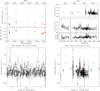 |
Fig. 1 Top panel: light curves of Cyg OB2 #5 and evolution of HR for XMM-Newton (left, pn in green, MOS1 in black, and MOS2 in red) and Swift data (right). Bottom panel: light curves folded with the two orbital periods of Cyg OB2 #5. XMM-Newton-pn data were divided by 10 and are shown as red stars, while Swift data are shown as black dots. On the left, quadratic ephemeris from Eq. (2) were used to derive the phase, while the ephemeris of the long orbit from Sect. 4.3 were used for the right panel. |
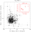 |
Fig. 2 Countrates compared to hardness ratios for Swift and XMM-Newton (in red, inset). For the XMM-Newton data, the vertical axis represents HR = (H + S)∕(H − S) rather than H∕S. |
4 Long-term optical monitoring
4.1 Photometry
The eclipses of the inner binary of Cyg OB2 #5 were first reported by Miczaika (1953). The primary eclipse (eclipse of the primary star by the secondary) is ~0.3 mag deep, whichis slightly more than the secondary eclipse which has a depth of ~0.25 mag. The eclipseshave been repeatedly observed since then and three types of information are available in the literature: (1) full datasets(Miczaika 1953; Hall 1974; Linder et al. 2009; Yaşarsoy & Yakut 2014; Kumsiashvili & Chargeishvili 2017; Laur et al. 2017, see also the Hipparcos, INTEGRAL Optical Monitoring Camera (OMC), and ASAS-SN databases6); (2) times of primary or secondary eclipses (Sazonov 1961; Häussler 1964; Romano 1969; Kurochkin 1985; Hubscher & Walter 2007; Zasche et al. 2017); and (3) light-curve modelling, often considering quadratic ephemeris (Hall 1974; Leung & Schneider 1978; Linder et al. 2009; Yaşarsoy & Yakut 2014; Laur et al. 2015; Antokhina et al. 2016).
The presence of Star C, a gravitationally bound companion to the inner, eclipsing binary should lead to light-time effects on the times of its photometric minima. These effects can be studied by comparing the observed times of primary minimum to those computed from the ephemeris of the eclipsing binary. To this aim, precise eclipse timing is needed. Unfortunately, discrepancies exist among the reported values. For example, Miczaika (1953) provided a primary eclipse time in Julian day of 2 434 265.73 whereas Hall (1974) quoted Miczaika’s time as 2 434 218.463; Kurochkin (1985) asserted that the eclipse times given by Miczaika (1953) and Sazonov (1961) are wrong while those of Romano (1969) deviate a lot from the ephemeris, suggesting they are all inaccurate. Yaşarsoy & Yakut (2014) also excluded some of the Romano (1969) times, although without justifying their decision to do so.
Given these problems, we rederived the primary eclipse times t0 and their uncertainties in a homogeneous way for all available data7. Long datasets were cut into smaller chunks, checking that the light-curve shape was indeed well sampled by individual subsets. Table 2 provides the considered time intervals and number of data points. No cleaning of the data was performed, except for the OMC datasets where some clear outliers exist8.
Using a χ2 criterion, we then searched for the primary eclipse times and magnitude offsets minimizing the deviations between the (folded) individual data points and the theoretical light curve of Linder et al. (2009). Our method is similar to the semi-automatic fitting procedure (AFP) used by Zasche et al. (2014). The steps in time and offsets were 2 × 10⁻⁴ d and 0.001 mag, respectively. Fitting offsets is necessary because some sources provide the magnitude of the star, whilst others provide its relative magnitude with respect to comparison stars. Moreover, the datasets use different filters that are not always perfectly calibrated to the standard V filter. Owing to the strong reddening, the observed spectral energy distribution of Cyg OB2 #5 is quite steep and the calibration of the magnitude outside eclipse is thus quite sensitive to the passband of the filter that was used. Yet, whilst this affects the zero point of the light curve, it does not impact its shape. Linder et al. (2009) indeed showed that light curves collected with narrow-band filters with central wavelengths ranging between 4686 and 6051 Å could all be fitted with the same synthetic light curve (see their Figs. 1 and 2). Hence, whilst different V -band filters have different zero points, the morphology of the light curve is identical, allowing us to perform the correlation with a single template. We note that individual errors on data points are available in all but two cases: from the standard deviations of points taken the same night, we found that typical errors are ~0.010 and 0.020 mag for data from Hall (1974) and Kumsiashvili & Chargeishvili (2017), respectively, and we used these values for the χ2 calculation.
Since the orbital period of the inner binary may vary with time, we performed this χ2 minimization considering periods ranging between 6.59777 and 6.59820 d, which bracket literature values, by steps of 10−5 d. We found that the minimum χ2 values do not depend on the period. In fact, the individual datasets are usually too short for such minute variation of the period to become detectable. However, this procedure allows us to assess how sensitive the best-fit parameters are and the resulting range of t0 values provides a first estimate of the uncertainty on t0.
As a second step, we derived an empirical photometric light curve consisting of normal points obtained by phase-folding all datasets using the best-fit individual t0 times and offsets and by performing a median in 50 phase bins. We then repeated the χ2 minimization procedure using this light curve as comparison. As could be expected, χ2 values were smaller than in previous cases and the best-fit t0/offset values were slightly different. Shifting the theoretical or empirical light curves also revealed in some cases the presence of several local minima in eclipse times. As an example of the adjustment of the phase-folded light curves we show the fit to the two epochs of new photometric measurements in Fig. 5.
To quantify the uncertainty on t0 we performed Monte Carlo simulations to account for the intrinsic variability. To do so, we proceeded in the following way. For each dataset, we first computed the residuals of the observed light curve over the Linder et al. (2009) model taken as a template. We then computed the Fourier periodogram of these residuals using the method of Heck et al. (1985) and Gosset et al. (2001). For the highest quality datasets this periodogram revealed power that decreased as a function of frequency, although there were no dominant peaks. This situation is reminiscent of the red noise that was found in various massive stars, including the massive binary HD 149 404 (Rauw et al. 2019). For lower quality data, the periodogram was typically dominated by white noise. We then used the characteristics of the Fourier periodogram as input to our Monte Carlo code (Rauw et al. 2019) to simulate 5000 synthetic light curves with the same temporal sampling as the actual data. These artificial light curves were again fitted with the Linder et al. (2009) model template and the resulting t0 and photometricoffsets were used to build the distributions of these parameters. In most cases, we find a nearly normal distribution for t0 resulting in σ values of about 0.01–0.02 d. In several cases however the distributions are asymmetric (e.g. strongly peaked witha wing extending mostly to one side) or display several peaks (due to local minima of the χ2). In those cases, the errors were enlarged so that the ± 1σ interval encompasses the two neighbouring minima; the resulting σ values are significantly larger and in the worst case up to 0.08 d.
All these tests were done to get a realistic value of the errors. Indeed, the light curves present some scatter around the eclipse variations that exceed the photometric errors on individual data points. This comes from the presence of intrinsic variability on top of the light curve of the eclipsing system (Linder et al. 2009), which is a major contributor to the uncertainties on the determination of the times of primary minimum. Hence the χ2 for the best-fit t0 and offset values are larger than expected. Using the usual χ2 + 1 method to derive 1σ errors therefore leads to underestimates. Comparing the scatter in eclipse times derived by shifting the two comparison curves for a set of periods as well as from the Monte Carlo simulations provides a more secure estimate, albeit with larger error values. To be as conservative as possible, we decided to adopt as the best estimate of the error on t0 the maximum of the uncertainty estimates between half of the full range of t0 values derived by the shifting method and the σ obtained in the Monte Carlo simulations. Table 2 yields the final, average values of the eclipse times, along with their errors. With these values at hand, we then computed the best-fit ephemerides. The best-fit linear ephemerides are written as
Revised times of primary photometric minimum resulting from the light-curve fitting
 (1)
(1)
We computed the residuals, labelled  in Fig. 6, of the t0 values. The Fourier periodogram of the
  residuals indicates significant power at low frequencies. The highest peak corresponds to a timescale of about 33 yr which is half the total duration spanned by the data. We concluded that there exist long-term trends on top of the linear ephemerides, most probably associated to the mass loss of the inner binary system (Singh & Chaubey 1986). To account for these long-term trends we thus considered quadratic ephemerides.
The best-fit quadratic ephemerides are written as
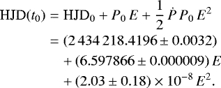 (2)
(2)
The quadratic ephemerides lead to a reduction of the χ2 of the fit from 89.2 (31 degrees of freedom) for Eq. (1) to 69.6 (30 degrees of freedom) for Eq. (2).
Compared to the quadratic ephemerides of Linder et al. (2009) and Laur et al. (2015), we find a value of Ṗ = (0.615 ± 0.055) 10−8 s s−1 = (0.19 ± 0.02) s yr−1, which is about one-third of the old value. The same reduction by a factor ~ 1∕3 applies to the mass-loss rate (computed according to case IV of Singh & Chaubey 1986) which would now be (7.7 ± 2.1) 10−6 M⊙ yr−1. The lower value of Ṗ is due to the much longer time series considered in this work, hence leading to a much better constrained value of Ṗ, and to the fact that we rederived the values of t0 in a self-consistent way rather than relying on published values. We note that this value of Ṁ is lower than that derived by Kennedy et al. (2010) from the thermal part of the radio emission, which was obtained assuming a larger distance than found by Gaia. The scaling of the result of Kennedy et al. (2010) is written as
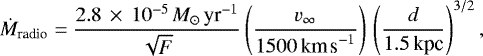 (3)
(3)
where F ≤ 1 stands for the volume filling factor. For reasonable values of F and v∞, the radio mass-loss rate appears thus larger than the optical value. However, in this comparison, we need to keep in mind that the primary radio component of Cyg OB2 #5 contains two wind interaction zones (between the winds of stars A and B and between the combined wind of stars A+B and the wind of Star C). Aside from the non-thermal radio emission that is seen to vary, these wind interaction zones can also contribute an extra thermal radio emission that could bias the determination of Ṁ from the radio flux towards higher values (Pittard 2010).
Figure 6 shows the residuals, labelled  , of the t0 values over the quadratic ephemerides; we then computed their Fourier periodogram (Fig. 7). For frequencies below 0.002 d−1, the highest peak is now present at a frequency9 of (0.0004227 ± 0.0000041) d−1, which corresponds to a period of (2366 ± 23) d or 6.48 yr. We note that this frequency is close to that of the second highest peak (at a frequency near 0.00038 d−1) in the periodogram of the
  data. This periodicity is interpreted in terms of reflex motion in Sect. 4.3. Finally, for completeness, Appendix B presents a detailed analysis of the combined light curve of the eclipsing binary.
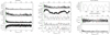 |
Fig. 3 Left panel: modified Fourier (with its spectral window on top), AOV, and conditional entropy periodograms considering all Swift data. Middle panel: modified Fourier periodograms for different sets of Swift data. Right, top panel: zoom on the low-frequency content of the modified Fourier periodogram calculated on all Swift data. Right, bottom panel: modified Fourier periodogram, with its spectral window, for Swift and XMM-Newton-pn data combined. The pn data were arbitrarily scaled by a factor 0.1. The two known periods (see also Sect. 4) are shown by dotted lines: green for 2366 d and red for 6.6 d. |
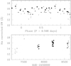 |
Fig. 4 Equivalent width of the Hα emission line measured on spectra collected with the HEROS spectrograph and corrected for the phase-locked variations of the continuum level. The data are shown as a function of orbital phase of the eclipsing binary (top panel, computed with the quadratic ephemerides, Eq. (2)) and as a function of date (bottom panel). Different symbols stand for different observing campaigns: crosses, open squares, filled triangles, filled circles and stars indicate data collected in 2015, 2016, 2017, 2018 and 2019, respectively. |
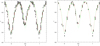 |
Fig. 5 Our new photometry folded with P = 6.59787 d and the best-fit eclipse times of Table 2. The green dashed curve corresponds to the theoretical light curve of Linder et al. (2009), whereas the red dotted curve corresponds to the empirical median light curve. Left and right panels:epochs (HJD-2 400 000) 58 262–58 333 and 58 358–58 426, respectively. |
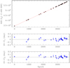 |
Fig. 6 Top panel: observed times of primary minimum as a function of epoch, along with the best-fit quadratic ephemerides (red line). Middle and bottom panels: O– C of the times of primary minimum as a function of epoch E for the linear ephemerides (middle panel) and the quadratic ephemerides (bottom panel). |
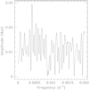 |
Fig. 7 Fourier periodogram of the |

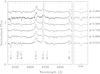 |
Fig. 8 Blue spectrum of Cyg OB2 #5 as a function of orbital phase as observed with the Aurélie spectrograph during our June 2014 OHP campaign. For clarity the consecutive spectra are shifted vertically by 0.3 continuum units. Right panel: zoom on the He II λ 4542 line. The blue and red tick marks above the spectra indicate the position of the primary and secondary absorptions, respectively, for those spectra where the lines were resolved. |
4.2 Spectroscopy
Figure 8 illustrates the phase dependence of the blue spectrum of Cyg OB2 #5 during our OHP campaign of 2014. Although the spectra clearly reveal the signature of the orbital motion of the eclipsing binary, assessing the nature and the properties of the components of this eclipsing binary is notoriously difficult. Indeed, as already noted by previous studies (e.g. Rauw et al. 1999), the visibility and nature of the absorption lines in the spectrum of Cyg OB2 #5 change considerably with orbital phase. For instance, the Hγ and He I λ 4471 lines display a P-Cygni type profile at phases around 0.35–0.55 and near phase 0.0. Whilst the orbital motion of the primary can clearly be traced by the RVs of the He II λλ 4542, 5412 and O III λ 5592 lines, measuring the RVs of the secondary is more difficult because of the appearance of P-Cygni absorption troughs at some orbital phases.
The spectrum also features a number of emission lines. Some of these emissions (Hα, He I λ 5876) arise mostly from the wind–wind collision zone (Rauw et al. 1999). Others, such as He II λ 4686, N III λλ 4634-40, Si IV λλ 4089, 4116, 6668, 6701 and S IV λλ 4486, 4504 closelyfollow the orbital motion of the secondary, although with a phase shift probably due to the contribution of a wind interaction region (Rauw et al. 1999). On the contrary, the C III λ 5696 emission follows the orbital motion of the primary.
Table A.3 lists our RV measurements of various absorption lines and of the peak of the He II λ 4686 emission. In Appendix C, we use these new RVs of the absorption lines to revise the orbital solution of the eclipsing binary. Unfortunately though, the RVs of the absorption lines are clearly not appropriate to detect a possible reflex motion of the eclipsing binary. Instead, we measured the RVs of the peak of the He II λ 4686 emission line. These RVs describe a sine wave that is slightly shifted in phase with respect to the RV curve of the secondary (see Rauw et al. 1999). This feature is most likely related to the wind–wind interaction in the eclipsing binary and turned out to be remarkably stable over more than two decades.
The red dots in Fig. 9 show the measured heliocentric velocities from Rauw et al. (1999) along with our new data folded with the quadratic ephemerides. The data were taken over 14 observing seasons (see Table 3). For each season, we adjusted an S-wave relation
 (4)
(4)
where the amplitude  was requested to be the same at all epochs. In this way, we thus obtained the values of the systemic velocity vz as a function of epoch (Table 3). We tested various values of the sine-wave amplitudes between 229 and 239 km s−1 and found stable values of the epoch-dependent vz velocities. The black dots in Fig. 9 indicate the RVs of the peak of He II λ 4686 after correcting for the variations of vz with epoch. Whilst the raw RVs have |O − C| = 16.9 km s−1 about the best-fit curve, the RVs corrected for the epoch dependence of vz have |O − C| = 13.6 km s−1. This may atfirst sight seem a small difference, but we show in next section its significance for the study of reflex motion.
4.3 Orbital signatures of Star C
Two observational pieces of evidence point towards the presence of reflex motion in the A+B system in Cyg OB2 #5 due to the presence of Star C: regularly changing eclipse times and changes in systemic velocities. Figure 10 shows the  data folded with the period of 2366 d. The modulation displays a peak-to-peak amplitude around 0.1 d. Provided we are dealing with a hierarchical triple system we can express the light-time effect as
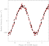 |
Fig. 9 Radial velocities of the peak of the He II λ 4686 emission line as a function of phase of the eclipsing binary. The orbital phases are computed with the quadratic ephemerides. The red dots yield the raw heliocentric RVs, whereas the black dots were corrected for the epoch-dependence of the systemic velocity. The best-fit S-wave relation (corresponding to vx = 28.8 km s−1, vy = 232.3 km s−1 and vz = 24.8 km s−1) is shown overplotted on the data. |
 (5)
(5)
where aAB, eAB+C, iAB+C, ϕAB+C(t) and ωAB indicate, respectively, the semi-major axis of the orbit of the A+B inner binary around the centre of mass of the A+B+C triple system, the eccentricity of this outer orbit, its inclination, the true anomalie at time t of the inner binary on the outer orbit, and the argument of periastron measured from the ascending node of the inner binary on the outer orbit.
We then folded the vz values with the 2366 d period (Fig. 10). Assuming they reflect an SB1 orbital motion, we can express them via
![Mathematical equation: \begin{eqnarray*} v_z(t) & = & v_{z,0} + \frac{a_{\textrm{AB}}\,\sin{i_{\textrm{AB+C}}}}{\sqrt{1 - e_{\textrm{AB+C}}^2}}\,\left(\frac{2\,\pi}{P_{\textrm{AB+C}}}\right)\,\left[\cos{(\phi_{\textrm{AB+C}}(t) + \omega_{\textrm{AB}})}\right. \nonumber \\ & & \left. + e_{\textrm{AB+C}}\,\cos{\omega_{\textrm{AB}}}\right].\end{eqnarray*}](/articles/aa/full_html/2019/07/aa35637-19/aa35637-19-eq13.png) (6)
(6)
Combining Eqs. (5) and (6), the orbital motion of the inner binary around centre of mass of the triple system can be described by five parameters: aAB siniAB+C, eAB+C, ωAB, vz,0 and tAB+C,0. The last of these parameters stands for the time of periastron passage of the outer orbit which is used along with PAB+C = 2366 d in Kepler’s equation to compute the true anomaly ϕAB+C(t). We searched for the combination of these five parameters that provides the best simultaneous fit to Eqs. (5) and (6). The best fit is illustrated in Fig. 10, and the 1σ and 90% confidence contours projected onto five parameter planes are shown in Fig. 11.
At the 1σ level, the best-fit parameters are  km s−1,
 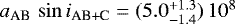 km,
km, 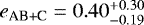 ,
, 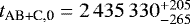 , and
, and 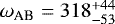 . Some parameters span a wide range of possible values. This is especially the case for eAB+C. Other parameters exhibit correlations (i.e., tAB+C,0 and ωAB). From these results, we can estimate the mass function of the outer orbit as
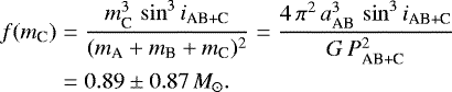 (7)
(7)
Considering the masses of the A and B components (see Appendix C) and the probable inclination of the orbit (see Sect. 5), we derive  M⊙, placing this star in the B-type range if it is a supergiant as the A and B components. Our value of mC is a factor 1.6 lower than the estimate of Kennedy et al. (2010), although both estimates overlap within their errors. Our best values of the orbital parameters are summarized in Table 4 along with those of the inner orbit (derived in Appendix C).
From the third light value found in Appendix B and accounting for the contributions from Star D, we can estimate a magnitude difference between Star C and the eclipsing binary of about 2.1. Whilst spectral lines associated to Star C could easily remain hidden in the complex A+B spectrum, a direct detection of Star C is certainly within the reach of modern long baseline interferometry. At a distance of 1.5 kpc, the semi-major axis of the tertiary orbit (13.2 AU) corresponds to an angular separation of 0.009′′. These parameters along with the near-infrared magnitude of Cyg OB2 #5 make it a promising target for the refurbished Center of High Angular Resolution Astronomy (CHARA) interferometric array. The most favourable time for detecting Star C via this technique would probably be around the next apastron passage, which is predicted for mid-August 2023.
Epoch-dependence of the systemic velocity of He II λ 4686.
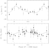 |
Fig. 10 Top: vz velocity of the peak of the He II λ 4686 emissionline as a function of epoch folded with the 2366 d period. Bottom: |

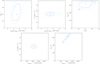 |
Fig. 11 χ2 contours of the combined fit of the 6.5 yr orbit corresponding to uncertainties of 1σ (blue contour) and the 90% confidence range (cyan contour) projected on planes consisting of various pairs of parameters. The best-fit solution is shown by the black dots. The magenta square (with error bars) in the third and fifth figure yields the parameters and their 1σ errors as determined from the fit of the radio light curve for s = 2 (see Sect. 5). |
Orbital parameters of the triple system in Cyg OB2 #5.
5 Revisiting the radio light curve
The first evidence for the presence of Star C in Cyg OB2 #5 came from radio observations. In this section, we revisit the published radio data in view of our optical results. We first folded the 4.8 and 8.4 GHz VLA data from Kennedy et al. (2010) and the 8.4 GHz VLBA data from Dzib et al. (2013) with our ephemerides. The VLBA data indicate fluxes that are significantly lower than those of the VLA observations. Dzib et al. (2013) estimated that about one-fourth of the non-thermal flux was resolved out by the VLBA. In addition, most of the more extended thermal fluxis also resolved out. To match the level of the two sets of data, we have thus multiplied the VLBA fluxes by a factor four-thirds and added 5 mJy. This scaling is somewhat arbitrary, and we include the VLBA data only for illustrative purpose. The results are shown in Fig. 12. Except for one strongly deviating VLBA point, our best-fit period of 2366 d yields a smooth radio light curve and allows us to reconcile the Kennedy et al. (2010) and Dzib et al. (2013) data. We also note that the radio minima coincide well with the time of periastron.
We then implemented the model of Kennedy et al. (2010), originally proposed by Williams et al. (1990), to describe the variations ofthe radio emission of Cyg OB2 #5. In this model, the observed radio flux (in mJy) is given by the sum of the constant free–free thermal emission of the wind and a phase-dependent non-thermal emission associated with the shock between the winds of A+B and C which undergoes a phase-dependent free-free absorption by the wind of A+B, i.e.
![Mathematical equation: \begin{equation*} S_{\nu}(t) = 2.5\,\left(\frac{\nu}{4.8\,\textrm{GHz}}\right)^{0.6} + S_{4.8}(t)\,\left(\frac{\nu}{4.8\,\textrm{GHz}}\right)^{\alpha}\,\exp{[-\tau_{\nu}(t)]}.\end{equation*}](/articles/aa/full_html/2019/07/aa35637-19/aa35637-19-eq21.png) (8)
(8)
In this equation, ν, S4.8, α, and τν (t) are the frequency (in GHz), the level of the non-thermal emission at 4.8 GHz, its spectral index, and the optical depth of the wind, respectively (Williams et al. 1990; Kennedy et al. 2010). We assumed that S4.8 (t) scales with the orbital separation as
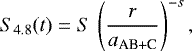 (9)
(9)
and that the optical depth varies with frequency as
 (10)
(10)
The optical depth τ4.8(t) is expressed as a function of time and of the orbital parameters (see Williams et al. 1990, and Appendix D).
We compared the radio fluxes of Kennedy et al. (2010) folded with our period to grids of synthetic radio light curves computed with Eq. (8). We computed four grids, corresponding to the values of s considered by Kennedy et al. (2010), i.e. 0.0, 0.5, 1.0, and 2.0. The parameter space spans seven dimensions as our grid samples eAB+C between 0.0 and 0.8 (21 steps), t0 with 100 steps of 0.01 PAB+C, ωC between 0 and 2 π (120 steps), τ0 between 0.4 and 4.0 (10 steps), α between − 1.1 and − 0.2 (10 steps), S between 6.0 and 13.0 mJy (15 steps), and iAB+C between 45° and 90° (4 steps).
Kennedy et al. (2010) found inclinations very close to 90°, although with rather large uncertainties. Our calculations confirmed this situation. Overall, the best-fit quality is obtained for s = 2.0. Considering all models that are acceptable at the 1σ level, we find the following parameters from the radio light curve: eAB+C = 0.215 ± 0.059,  , tAB+C,0 = 34909 ± 90, τ0 = 3.11 ± 0.68, α = −0.80 ± 0.14, S = (10.50 ± 1.65) mJy, and
  . The synthetic curves corresponding to these parameters are shown on top of the observations in Fig. 12 and some parameters and their errors are shown in Fig. 11. We find a fair agreement between the two totally independent determination of those parameters (eAB+C, ωAB+C, tAB+C,0) that are in common with the orbit determination in Sect. 4.3. This further supports our determination of the properties of Star C.
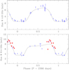 |
Fig. 12 Radio fluxes of Cyg OB2 #5 as a function of phase in the 2366 d cycle (with tAB+C,0 = 34909) along with the best-fit model with s = 2 (see text). The crosses stand for the VLA data from Kennedy et al. (2010), whereas the filled dots indicate the VLBA fluxes from Dzib et al. (2013) multiplied by a factor 4/3 and with a 5 mJy offset added (see text). The VLBA data were not used in the fit but they nevertheless agree well with VLA results. |
6 Discussion and conclusions
Cyg OB2 #5 is a highly interesting, but extremely challenging massive multiple system. In particular, previous radio studies of the system hinted at the possible presence of a star orbiting the inner binary, which remained to be confirmed. In this context, a number of open issues exist, notably on the exact nature of the radio and X-ray emission.
Using photometric data spanning more than six decades, we have shown for the first time that there exists a light-time effect in the times of primary eclipses of the innermost binary. This indicates a periodic motion with a period of 6.5 yr. We further found the signature of this reflex motion in the systemic velocity of the He II λ 4686 emission line. Whilst the orbital parameters are still subject to relatively large uncertainties, we note that they favour a moderate eccentricity. Folding the radio data with our newly determined period, we found that they are best fitted with a model where the intrinsic non-thermal radio emission from the wind interaction zone falls off with orbital separation as r−2.
Concerning the X-ray emission, we found considerable variability on timescales of months, but no clear indication of a phase-locked variability with either the period of the eclipsing binary or the 6.5 yr period of the triple system. Though the X-ray overluminosity of Cyg OB2 #5 most likely stems from the existence of several wind interaction zones in this system, the variability cannot be directly connected to the orbital phases of the A+B or AB+C systems and thus seems to have different origins. We tentatively suggest that transient variations of the mass-loss rate of the eclipsing binary might be responsible for part of these changes of the X-ray emission.
Future work, notably using a proper treatment of atmospheric eclipses, may further shed light on the exact nature of Star B and the remaining discrepancy in distance estimate (see Appendix B).
Acknowledgements
We acknowledge support from the Fonds National de la Recherche Scientifique (Belgium), the Communauté Française de Belgique (including notably support for the observing runs at OHP), the European Space Agency (ESA) and the Belgian Federal Science Policy Office (BELSPO) in the framework of the PRODEX Programme (contract XMaS). G.R. acknowledges the continuous efforts of the administration of Liège University, especially the finance department, to make his life more complicated. We thank the Swift team for their kind assistance as well as Drs Yakut, Laur, and Paschke for their help in locating data. Our thanks also go to Dietmar Bannuscher and Klaus Häußler for providing us with a copy of the Harthaer Beobachtungszirkulare and to Dr P.M. Williams for advices on the modelling of the radio light curve. We thank Dr Zasche for his constructive referee report. ADS and CDS were used for this research.
Appendix A Journal of X-ray and optical spectroscopy observations
In this appendix, we provide the detailed list of the XMM-Newton and Swift observations of Cyg OB2 #5 (Tables A.1 and A.2), as well as the list of the new optical spectra and the corresponding RVs (Table A.3).
Journal of the XMM-Newton observations.
Journal of the Swift observations.
Journal of the new RV measurements of the eclipsing binary.
Appendix B Analysis of the light curve of the eclipsing binary
As pointed out above, we combined all the available photometric measurements to construct an empirical V -band light curve consisting of points which are obtained by taking the median of the data in 50 equally spaced phase bins. Unlike the original data, this empirical light curve is essentially free of intrinsic variability. We thus took advantage of this light curve to perform a new photometricsolution of the eclipsing binary with the nightfall code (version 1.86) developed by R. Wichmann, M. Kuster and P. Risse10 (Wichmann 2011). This code relies on the Roche potential to describe the shape of the stars. For the simplest cases (two stars on a circular orbit with neither stellar spots nor discs), the model is thus fully described by six parameters: the mass-ratio, the orbital inclination, the primary and secondary filling factors (defined as the ratio of the stellar polar radius to the polarradius of the associated Roche lobe), and the primary and secondary effective temperatures. We set the mass-ratio to 3.2 and the stellar effective temperatures to 36 000 K. Following Antokhina et al. (2016), we adopted a square-root limb-darkening law. Reflection effects were accounted for by considering the mutual irradiation of all pairs of surface elements of the two stars (Hendry & Mochnacki 1992). In accordance with Linder et al. (2009), we found that including a bright spot on the secondary star significantly improves the quality of the fits.
Previous photometric solutions, not accounting for the presence of third light, yielded orbital inclinations in the range from 64° to 68° (Leung & Schneider 1978; Linder et al. 2009; Yaşarsoy & Yakut 2014; Laur et al. 2015; Antokhina et al. 2016). As shown by Cazorla et al. (2014), accounting for a third light contribution leads to higher inclinations. Third light arises from components C and D. According to Mason et al. (2001), Star D is 2.5 mag fainter than the combination of A, B and C (assuming that the Mason et al. 2001 magnitude refers to the maximum light of the eclipsing binary). This implies that the third light contribution from Star D should be lD ∕(lA + lB + lC + lD) ≤ 0.1. Our best-fit parameters for the V -band light curve (Table B.1) hence suggest a third light contribution due to star C around lC ∕(lA + lB + lC + lD) ~ 0.13.
In line with previous studies (Leung & Schneider 1978; Linder et al. 2009; Yaşarsoy & Yakut 2014; Laur et al. 2015; Antokhina et al. 2016), we can achieve a reasonable fit of the light curve for an overcontact configuration (see Fig. B.1). Yet, whilst the fit looks reasonable, there are two major problems which remain unsolved: the conflict between the visual brightness ratio inferred from photometry and spectroscopy, and the distance problem.
The light-curve solutions that we obtained yield a visual brightness ratio of 3.6 ± 0.4 between the primary and secondary star. This value is significantly larger than the brightness ratio near 1.4 inferred from the strengths of the primary and secondary spectral lines (Rauw et al. 1999).
Hall (1974) quoted mV = 9.05 and B–V = 1.72 outside eclipses. This is in good agreement with the zero points of the photometric data in our analysis which suggest mV = 9.10 ± 0.05 outside eclipse. We thus adopt mV = 9.10 ± 0.05 and B– V = 1.72 ± 0.07 outside eclipse, along with  (Martins & Plez 2006) and RV = 3.0 (Massey & Thompson 1991), resulting in AV = 5.97 ± 0.21. With the Gaia-DR2 distance modulus of
  (Bailer-Jones et al. 2018), we thus estimate an absolute magnitude of
  . Adopting the bolometric corrections from Martins & Plez (2006), we can convert the parameters of the best-fitting nightfall models into an absolute magnitude of MV,model = −7.33 ± 0.10. This value is significantly fainter than the Gaia-DR2 absolute magnitude, indicating that we are missing about one-third of the total flux of the system.
Parameters of the best fit with nightfall to the V -band light curve ofCyg OB2 #5.
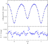 |
Fig. B.1 Best-fit nightfall solution of the V -band light curve of Cyg OB2 #5. The model parameters are given in Table B.1. In the model, the secondary features a bright spot on the side facing the primary. |
A possible solution to the distance problem could be a higher temperature and thus higher luminosity of the primary star. Yet, we emphasize that the strength of the primary’s He I λ 4471 line relative to that of the He II λ 4542 line is fully compatible with an O6.5-7 spectral type for the primary, although this conclusion could be somewhat affected by blends with spectral features of Star C. We further note that the spectra display no N V λλ 4604, 4620 absorptions, indicating a spectral type later than O4 (Walborn et al. 2002) and thus a temperature < 40 000 K. Therefore, the primary temperature is unlikely to significantly exceed 36 000 K. The interstellar absorption towards Cyg OB2 is very large. Whilst our values of E(B − V) and AV are in line with other determinations (Leitherer et al. 1982; Massey & Thompson 1991; Hanson 2003), Torres-Dodgen et al. (1991) derived a higher value of AV = 6.40. Adopting this value of the visual extinction would worsen the distance problem as it would bring the discrepancy between the two absolute magnitude estimates to 0.85 mag instead of 0.42 mag.
The distance problem would disappear if the secondary were as bright as the primary in the V band, which is actually what the spectroscopic data suggest. However, this is clearly at odds with the light-curve analysis. The unequal eclipse depths indicate a primary star that should be hotter than the secondary. Therefore, to have similar optical brightnesses, the secondary should be at least as big as the primary. This is clearly not possible for a contact or overcontact configuration with q = mA∕mB = 3.1.
As pointed out above, the light-curve model assumes that the shape of the stars is given by the Roche potential. Antokhina et al. (2016) suggested that the presence of an accretion disc around one of the components of the eclipsing binary could affect the light curve. Yet, Doppler tomography of the Hα and He II λ 4686 emission lines revealed no evidence of a disc-like structure around any of the stars (Linder et al. 2009). Therefore, there is no observational justification for including such a disc in the photometric solution. Alternatively, the presence of a strong wind around one of the components could also affect the light curve via the formation of atmospheric eclipses. As shown by Anthokhina et al. (2013), optically thick stellar winds can lead to non-equal eclipse depths for stars that have otherwise identical properties. There are some indications in favour of such a scenario. We can first cite the large difference of the systemic velocities between the primary and secondary star (see Table C.1 and Fig. C.1), as well as the shift in systemic velocity between different lines and compared to the systemic velocities of other early-type binaries in Cyg OB2 (Kobulnicky et al. 2014). These results indicate that both stars have a strong stellar wind, and that the secondary wind is probably denser than that of the primary. Further support comes from the appearance of variable P-Cygni type profiles at certain orbital phases. Atmospheric eclipses can indeed result in variable absorption troughs of P-Cygni profiles (Auer & Koenigsberger 1994). At first sight, because of the wavelength-dependence of the opacity, we would expect a stellar wind to produce light curves with differences in morphology as a function of wavelength. This is best probed with narrow-band filters that mainly encompass continuum versus filters that specifically focus on wind emission lines. Such a set of filters was used by Linder et al. (2009). Whereas the He II λ 4686 line-bearing filter showed no strong deviation from the continuum filters, significant differences were found for the He I λ 5876 line-bearing filter. Whilst the former result suggests that the opacity of the He II λ 4686 line in the wind does not exceed that of the continuum, the latter situation was explained by Linder et al. (2009) as a consequence of the variable He I λ 5876 P-Cygni absorption trough. The most likely picture is thus that of a secondary wind that is optically thick in the continuum (due to free electron scattering; Anthokhina et al. 2013), as is the case for Wolf-Rayet stars. Under such circumstances, the “pseudo-photosphere” of the secondary might actually extend beyond the size of the Roche equipotential filled by the hydrostatic core of the secondary star.
From the above considerations, we see that both issues of the photometric solution could possibly be solved via the inclusion of the wind absorption into the model. Including wind parameters (mass-loss rate, wind terminal velocity and velocity law) introduces however a number of degeneracies (Anthokhina et al. 2013). Designing an algorithm to solve the light curve accounting for the effects of the stellar wind and overcoming the limitations of these degeneracies is a long and strenuous task unrelated to the goal of this paper and that we defer to future work.
Appendix C Revised orbital solution of the eclipsing binary
We used our newly determined RVs (Table A.3) along with the quadratic ephemerides (Eq. (2)) to revise the orbital solution of the inner binary system. For the primary star, the He II λ 5412 and O III λ 5592 lines consistently yield a semi-amplitude of the RV curve of KA ~ 88 km s−1 (see Fig. C.1). This value is about seven percent larger than the semi-amplitude inferred for the same lines by Rauw et al. (1999), although the results overlap within the error bars. The RVs of the He I λ 4471 and He II λ 4542 lines of the primary yield larger values of KA (between 110 and 115 km s−1). The dispersion of the data points around the best-fit RV curve is larger for those two lines. These differences in K and their dispersion certainly reflect the difficulties due to the lines displaying P-Cygni type profiles at some orbital phases. For the secondary, the cleanest results are obtained from the RVs of the He II λ 5412 line. This line yields KB ~ 325 km s−1. Unfortunately, because of the change in line morphology around phase 0.25, our new secondary RV measurements are extremely scarce at this phase and this situation could bias our determination of KB. Indeed, the He I λ 4471 and He II λ 4542 lines yield KB values of 261 and 255 km s−1, respectively. In view of these uncertainties, we thus adopted KA = (87.7 ± 6.1) km s−1 from the He II λ 5412 and O III λ 5592 RVs, and KB = (280 ± 31) km s−1, i.e. the average of the KB values of the three spectral lines for which the second component can be measured. The mass-ratio hence becomes 3.2 ± 0.4, whilst the minimum masses of the primary and secondary stars are mA sin3iA+B = (25.8 ± 8.6)M⊙ and mB sin3iA+B = (8.1 ± 1.9)M⊙, respectively. The corresponding projected orbital separation is aA+B siniA+B = (47.8 ± 4.0)R⊙.
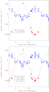 |
Fig. C.1 Radial velocity curves of the eclipsing binary. The orbital phases were computed with the quadratic ephemerides (Eq. (2)). Top panel: results obtained from the He II λ 5412 and O III λ 5592 RVs. Blue symbols stand for the primary star, whilst red symbols indicate the secondary. The primary RVs of O III λ 5592 were shifted to match the systemic velocity of the He II λ 5412 line (see Table C.1). The solid and dashed curves correspond to the best-fit orbital solution based on this line. Bottom panel: full set of RV measurements along with the preferred RV curves (see Table 4). For each star, the RVs of the various lines were shifted to match the systemic velocities of the He II λ 5412 line. |
Apparent systemic velocities of the absorption lines of Cyg OB2 #5.
We note that the different lines yield different apparent systemic velocities (see Table C.1). This situation probably reflects the presence of optically thick stellar winds, especially for the secondary star.
The revised orbital solution is shown in Fig. C.1 and summarized in Table 4. Although the errors on the revised orbital solution are larger than for the solution of Rauw et al. (1999), the new solution is to be preferred. In fact, the errors now account for the uncertainties related to the choice of the lines in the orbital solution, whilst this was not the case in the solution of Rauw et al. (1999).
Appendix D Expression of the free–free optical depth towards a point-like source
Williams et al. (1990) provided expressions for the free–free optical depth τ4.8(t) as a function of the orbital parameters. These authors used expressions that include the tangent of the orbital inclination. Yet, for inclinations near 90°, it is advantageous to use expressions that involve the cotangent of the orbital inclination instead. In this appendix, we provide these expressions.
For an orbital inclination iAB+C = 90°, we have
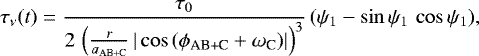 (D.1)
(D.1)
where τ0 is a fitting parameter, ωC = ωAB − π and ψ1 is given by
![Mathematical equation: \begin{align}&\psi_1 = \frac{\pi}{2} + (\phi_{\textrm{AB+C}} + \omega_{\textrm{C}}), \ \ \ \ \textrm{if}\ \ (\phi_{\textrm{AB+C}} + \omega_{\textrm{C}}) \in \left[0,\frac{\pi}{2}\right],\\ &\psi_1 = \frac{3\,\pi}{2} - (\phi_{\textrm{AB+C}} + \omega_{\textrm{C}}), \ \ \textrm{if}\ \ (\phi_{\textrm{AB+C}} + \omega_{\textrm{C}}) \in \left[\frac{\pi}{2},\frac{3\,\pi}{2}\right],\\ &\psi_1 = (\phi_{\textrm{AB+C}} + \omega_{\textrm{C}}) - \frac{3\,\pi}{2}, \ \ \textrm{if} \ \ (\phi_{\textrm{AB+C}} + \omega_{\textrm{C}}) \in \left[\frac{3\,\pi}{2},2\,\pi\right].\nonumber\\ \end{align}](/articles/aa/full_html/2019/07/aa35637-19/aa35637-19-eq30.png)
For an orbital inclination iAB+C < 90°, we obtain
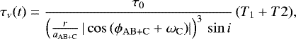 (D.5)
(D.5)
where
![Mathematical equation: \begin{equation*} T_1 = \frac{C'}{2\,\theta^3\,A'^{3/2}}\,\left[\textrm{arctan}{\left(\frac{2\,A'\,x+B'}{2\,\sqrt{A'}\,\theta}\right)}-\textrm{arctan}{\left(\frac{B'}{2\,\sqrt{A'}\,\theta}\right)}\right],\end{equation*}](/articles/aa/full_html/2019/07/aa35637-19/aa35637-19-eq32.png) (D.6)
(D.6)
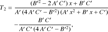 (D.7)
(D.7)
with
 (D.8)
(D.8)
 (D.9)
(D.9)
 (D.10)
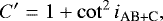 (D.11)
 (D.12)
and ψ1 has the same definition as above. Attention must be paid in the expression of T1 (Eq. (D.6)) to substitute  by
by  when the arctangent becomes negative.
References
- Antokhina, E. A., Antokhin, I. I., & Cherepashchuk, A. M. 2013, Astron. Astrophys. Trans., 28, 3 [NASA ADS] [Google Scholar]
- Antokhina, E. A., Kumsiashvili, M. I., & Chargeishvili, K. B. 2016, Astrophysics, 59, 68 [NASA ADS] [CrossRef] [Google Scholar]
- Auer, L. H., & Koenigsberger, G. 1994, ApJ, 436, 859 [NASA ADS] [CrossRef] [Google Scholar]
- Bailer-Jones, C. A. L., Rybizki, J., Fouesneau, M., Mantelet, G., & Andrae, R. 2018, AJ, 156, 58 [NASA ADS] [CrossRef] [Google Scholar]
- Bohannan, B., & Conti, P. S. 1976, ApJ, 204, 797 [NASA ADS] [CrossRef] [Google Scholar]
- Cazorla, C., Nazé, Y., & Rauw, G. 2014, A&A, 561, A92 [NASA ADS] [CrossRef] [EDP Sciences] [Google Scholar]
- Cincotta, P. M. 1999, MNRAS, 307, 941 [NASA ADS] [CrossRef] [Google Scholar]
- Cincotta, P. M., Helmi, A., Mendez, M., Nunez, J. A., & Vucetich, H. 1999, MNRAS, 302, 582 [NASA ADS] [CrossRef] [Google Scholar]
- Contreras, M. E., Rodríguez, L. F., Tapia, M., et al. 1997, ApJ, 488, L153 [NASA ADS] [CrossRef] [Google Scholar]
- Cuypers, J. 1987, Mededelingen van de Koninklijke academie voorWetenschappen, Letteren en Schone Kunsten van België, Academiae Analecta, 49, 3 [Google Scholar]
- De Becker, M., Rauw, G., Sana, H., et al. 2006, MNRAS, 371, 1280 [NASA ADS] [CrossRef] [Google Scholar]
- Dzib, S. A., Rodríguez, L. F., Loinard, L., et al. 2013, ApJ, 763, 139 [NASA ADS] [CrossRef] [Google Scholar]
- Gaia Collaboration (Brown, A.G.A, et al.) 2018, A&A, 616, A1 [NASA ADS] [CrossRef] [EDP Sciences] [Google Scholar]
- Gillet, D., Burnage, R., Kohler, D., et al. 1994, A&AS 108, 181 [NASA ADS] [Google Scholar]
- Gosset, E., & Nazé, Y. 2016, A&A, 590, A113 [NASA ADS] [CrossRef] [EDP Sciences] [Google Scholar]
- Gosset, E., Royer, P., Rauw, G., Manfroid, J., & Vreux, J.-M. 2001, MNRAS, 327, 435 [NASA ADS] [CrossRef] [Google Scholar]
- Graham, M. J., Drake, A. J., Djorgovski, S. G., Mahabal, A. A., & Donalek, C. 2013, MNRAS, 434, 2629 [NASA ADS] [CrossRef] [Google Scholar]
- Hall, D. S. 1974, Acta Astron., 24, 69 [NASA ADS] [Google Scholar]
- Hanson, M. M. 2003, ApJ, 597, 957 [NASA ADS] [CrossRef] [Google Scholar]
- Harnden, F. R., Jr. Branduardi, G., Elvis, M., et al. 1979, ApJ, 234, L51 [NASA ADS] [CrossRef] [Google Scholar]
- Häussler K., Harthaer Beobachtungs-Zirkular (HBZ), #23 [Google Scholar]
- Heck, A., Manfroid, J., & Mersch, G. 1985, A&AS, 59, 63 [NASA ADS] [Google Scholar]
- Hendry, P. D., & Mochnacki, S. W. 1992, ApJ, 399, 603 [NASA ADS] [CrossRef] [Google Scholar]
- Hinkle, K., Wallace, L., Valenti, J., & Harmer, D. 2000, Visible and Near Infrared Atlas of the Arcturus Spectrum 3727-9300 A, eds. K. Hinkle, L. Wallace, J. Valenti, & D. Harmer (San Francisco: ASP) [Google Scholar]
- Hubscher, J., & Walter, F. 2007, IBVS, 5761, 1 [NASA ADS] [Google Scholar]
- Jurkevich, I. 1971, Ap&SS, 13, 154 [NASA ADS] [CrossRef] [Google Scholar]
- Kennedy, M., Dougherty, S. M., Fink, A., & Williams, P. M. 2010, ApJ, 709, 632 [NASA ADS] [CrossRef] [Google Scholar]
- Kobulnicky, H. A., Kiminki, D. C., Lundquist, M. J., et al. 2014, ApJS, 213, 34 [NASA ADS] [CrossRef] [Google Scholar]
- Kumsiashvili, M. I., & Chargeishvili, K. B. 2017, Astrophysics, 60, 165 [NASA ADS] [CrossRef] [Google Scholar]
- Kurochkin, N. E. 1985, Peremennye Zvezdy, 22, 219 [NASA ADS] [Google Scholar]
- Laur, J., Tempel, E., Tuvikene, T., Eenmäe, T., & Kolka, I. 2015, A&A, 581, A37 [NASA ADS] [CrossRef] [EDP Sciences] [Google Scholar]
- Laur, J., Kolka, I., Eenmäe, T., Tuvikene, T., & Leedjärv, L. 2017, A&A, 598, A108 [NASA ADS] [CrossRef] [EDP Sciences] [Google Scholar]
- Leitherer, C., Hefele, H., Stahl, O., & Wolf, B. 1982, A&A, 108, 102 [NASA ADS] [Google Scholar]
- Leung, K.-C., & Schneider, D. P. 1978, ApJ, 224, 565 [NASA ADS] [CrossRef] [Google Scholar]
- Linder, N., Rauw, G., Manfroid, J., et al. 2009, A&A, 495, 231 [NASA ADS] [CrossRef] [EDP Sciences] [Google Scholar]
- Lomax, J. R., Nazé, Y., Hoffman, J. L., et al. 2015, A&A, 573, A43 [NASA ADS] [CrossRef] [EDP Sciences] [Google Scholar]
- Martins, F., & Plez, B., 2016 A&A, 457, A637 [Google Scholar]
- Mason, B. D., Wycoff, G. L., Hartkopf, W. I., Douglass, G. G., & Worley, E. 2001, AJ, 122, 3466 [Google Scholar]
- Massey, P., & Conti, P. S. 1977, ApJ, 218, 431 [NASA ADS] [CrossRef] [Google Scholar]
- Massey, P., & Thompson, A. B. 1991, AJ, 101, 1408 [NASA ADS] [CrossRef] [Google Scholar]
- Miczaika, G. R. 1953, PASP, 65, 141 [NASA ADS] [CrossRef] [Google Scholar]
- Miralles, M. P., Rodríguez, L. F., Tapia, M., et al. 1994, A&A, 282, 547 [NASA ADS] [Google Scholar]
- Mittag, M., Hempelmann, A., González-Pérez, J. N., & Schmitt, J. H. M. M. 2010, Adv. Astron. 101502 [Google Scholar]
- Nazé, Y., Mahy, L., Damerdji, Y., et al. 2012, A&A, 546, A37 [NASA ADS] [CrossRef] [EDP Sciences] [Google Scholar]
- Ortiz-León, G. N., Loinard, L., Rodríguez, L. F., Mioduszewski, A. J., & Dzib, S. A. 2011, ApJ, 737, 30 [NASA ADS] [CrossRef] [Google Scholar]
- Pandey, J. C., Pandey, S. B., & Karmakar, S. 2014, ApJ, 788, 84 [NASA ADS] [CrossRef] [Google Scholar]
- Pittard, J. M. 2010, MNRAS, 403, 1657 [NASA ADS] [CrossRef] [Google Scholar]
- Qian, S.-B., Kreiner, J. M., Liu, L., et al. 2007, Binary Stars as Critical Tools & Tests in Contemporary Astrophysics (Cambridge: Cambridge University Press), Proc. IAU Symp., 240, 331 [NASA ADS] [Google Scholar]
- Rauw, G. 2011, A&A, 536, A31 [NASA ADS] [CrossRef] [EDP Sciences] [Google Scholar]
- Rauw, G., & Nazé, Y. 2016, Adv. Space Res., 58, 761 [NASA ADS] [CrossRef] [Google Scholar]
- Rauw, G., Vreux, J.-M., & Bohannan, B. 1999, ApJ, 517, 416 [NASA ADS] [CrossRef] [Google Scholar]
- Rauw, G., Mahy, L., Nazé, Y., et al. 2014, A&A, 566, A107 [NASA ADS] [CrossRef] [EDP Sciences] [Google Scholar]
- Rauw, G., Pigulski, A., Nazé, Y., et al. 2019, A&A, 621, A15 [NASA ADS] [CrossRef] [EDP Sciences] [Google Scholar]
- Romano, G. 1969, Mem. Soc. Astron. It., 40, 375 [NASA ADS] [Google Scholar]
- Sazonov, V. 1961, Peremennye Zvezdy, 13, 445 [NASA ADS] [Google Scholar]
- Scargle, J. D. 1982, ApJ, 263, 835 [NASA ADS] [CrossRef] [Google Scholar]
- Schmitt, J. H. M. M., Schröder, K.-P., Rauw, G., et al. 2014, Astron. Nachr., 335, 787 [NASA ADS] [CrossRef] [Google Scholar]
- Schwarzenberg-Czerny, A. 1989, MNRAS, 241, 153 [NASA ADS] [CrossRef] [Google Scholar]
- Singh, M., & Chaubey, U. S. 1986, Ap&SS 124, 389 [NASA ADS] [CrossRef] [Google Scholar]
- Stellingwerf, R. F. 1978, ApJ, 224, 953 [NASA ADS] [CrossRef] [Google Scholar]
- Torres-Dodgen, A.V., Tapia, M., & Carroll, M. 1991, MNRAS, 249, 1 [NASA ADS] [CrossRef] [Google Scholar]
- Vreux, J.-M. 1985, A&A, 143, 209 [NASA ADS] [Google Scholar]
- Walborn, N. R., Howarth, I. D., Lennon, D. J., et al. 2002, AJ, 123, 2754 [NASA ADS] [CrossRef] [Google Scholar]
- Whittaker, E. T., & Robinson, G. 1944, The calculus of observations; a treatise on numerical mathematics, eds. E. T. Whittaker & G. Robinson (London: Blackie) [Google Scholar]
- Wichmann, R. 2011, Astrophysics Source Code Library [record ascl:1106.016] [Google Scholar]
- Williams, P. M., van der Hucht, K. A., Pollock, A. M. T., et al. 1990, MNRAS, 243, 662 [NASA ADS] [Google Scholar]
- Willis, A. J., Schild, H., & Stevens, I. R. 1995, A&A, 298, 549 [NASA ADS] [Google Scholar]
- Yaşarsoy, B.,& Yakut, K. 2014, New Astron., 31, 32 [NASA ADS] [CrossRef] [Google Scholar]
- Yoshida, M., Kitamoto, S., & Murakami, H. 2011, PASJ, 63, S717 [NASA ADS] [Google Scholar]
- Zasche, P., Wolf, M., Vraštil, J., et al. 2014, A&A, 572, A71 [NASA ADS] [CrossRef] [EDP Sciences] [Google Scholar]
- Zasche, P., Uhlar, R., Svoboda, P., et al. 2017, IBVS, 6204, 1 [NASA ADS] [Google Scholar]
- Zechmeister, M., & Kürster, M. 2009, A&A, 496, 577 [NASA ADS] [CrossRef] [EDP Sciences] [Google Scholar]
Throughout this paper, we adopt the naming convention of Kennedy et al. (2010) which is different from that used in the Washington Double Star Catalog (Mason et al. 2001).
This actually confirmed an early periodicity detection in the system from Miralles et al. (1994).
SAS threads, see http://xmm.esac.esa.int/sas/current/documentation/threads/
These papers also note that the method of Scargle (1982), while popular, is not fully correct, statistically.
Available from Vizier catalogue I/239/hip_va_1, http://sdc.cab.inta-csic.es/omc/ and https://asas-sn.osu.edu/, respectively; the few data from the Northern Survey for Variable Stars do not well cover the light curve.
Unfortunately, many publications only provide the value of t0 and do not quote the original photometric data on which the analysis was based. For these references it is impossible to establish an estimate of the uncertainty on t0.
Points that were kept have V < 9.45 for all phases and V < 9.35 in ϕ = 0.1–0.2, V < 9.2 in ϕ = 0.2–0.4, V < 9.35 in ϕ = 0.4–0.65, V < 9.2 in ϕ = 0.65–0.7, V < 9.15 in ϕ = 0.7–0.85, V < 9.2 in ϕ = 0.85–0.9.
Inspecting the periodogram at higher frequencies, we noted several peaks of similar strength. However, they correspond to timescales of less than 500 d, which are actually not well sampled by our
 data.
data.
The code is available at: http://www.hs.uni-hamburg.de/DE/Ins/Per/Wichmann/Nightfall.html
All Tables
Revised times of primary photometric minimum resulting from the light-curve fitting
Parameters of the best fit with nightfall to the V -band light curve ofCyg OB2 #5.
All Figures
|
Fig. 1 Top panel: light curves of Cyg OB2 #5 and evolution of HR for XMM-Newton (left, pn in green, MOS1 in black, and MOS2 in red) and Swift data (right). Bottom panel: light curves folded with the two orbital periods of Cyg OB2 #5. XMM-Newton-pn data were divided by 10 and are shown as red stars, while Swift data are shown as black dots. On the left, quadratic ephemeris from Eq. (2) were used to derive the phase, while the ephemeris of the long orbit from Sect. 4.3 were used for the right panel. |
| In the text | |
|
Fig. 2 Countrates compared to hardness ratios for Swift and XMM-Newton (in red, inset). For the XMM-Newton data, the vertical axis represents HR = (H + S)∕(H − S) rather than H∕S. |
| In the text | |
|
Fig. 3 Left panel: modified Fourier (with its spectral window on top), AOV, and conditional entropy periodograms considering all Swift data. Middle panel: modified Fourier periodograms for different sets of Swift data. Right, top panel: zoom on the low-frequency content of the modified Fourier periodogram calculated on all Swift data. Right, bottom panel: modified Fourier periodogram, with its spectral window, for Swift and XMM-Newton-pn data combined. The pn data were arbitrarily scaled by a factor 0.1. The two known periods (see also Sect. 4) are shown by dotted lines: green for 2366 d and red for 6.6 d. |
| In the text | |
|
Fig. 4 Equivalent width of the Hα emission line measured on spectra collected with the HEROS spectrograph and corrected for the phase-locked variations of the continuum level. The data are shown as a function of orbital phase of the eclipsing binary (top panel, computed with the quadratic ephemerides, Eq. (2)) and as a function of date (bottom panel). Different symbols stand for different observing campaigns: crosses, open squares, filled triangles, filled circles and stars indicate data collected in 2015, 2016, 2017, 2018 and 2019, respectively. |
| In the text | |
|
Fig. 5 Our new photometry folded with P = 6.59787 d and the best-fit eclipse times of Table 2. The green dashed curve corresponds to the theoretical light curve of Linder et al. (2009), whereas the red dotted curve corresponds to the empirical median light curve. Left and right panels:epochs (HJD-2 400 000) 58 262–58 333 and 58 358–58 426, respectively. |
| In the text | |
|
Fig. 6 Top panel: observed times of primary minimum as a function of epoch, along with the best-fit quadratic ephemerides (red line). Middle and bottom panels: O– C of the times of primary minimum as a function of epoch E for the linear ephemerides (middle panel) and the quadratic ephemerides (bottom panel). |
| In the text | |
|
Fig. 7 Fourier periodogram of the |
| In the text | |
|
Fig. 8 Blue spectrum of Cyg OB2 #5 as a function of orbital phase as observed with the Aurélie spectrograph during our June 2014 OHP campaign. For clarity the consecutive spectra are shifted vertically by 0.3 continuum units. Right panel: zoom on the He II λ 4542 line. The blue and red tick marks above the spectra indicate the position of the primary and secondary absorptions, respectively, for those spectra where the lines were resolved. |
| In the text | |
|
Fig. 9 Radial velocities of the peak of the He II λ 4686 emission line as a function of phase of the eclipsing binary. The orbital phases are computed with the quadratic ephemerides. The red dots yield the raw heliocentric RVs, whereas the black dots were corrected for the epoch-dependence of the systemic velocity. The best-fit S-wave relation (corresponding to vx = 28.8 km s−1, vy = 232.3 km s−1 and vz = 24.8 km s−1) is shown overplotted on the data. |
| In the text | |
|
Fig. 10 Top: vz velocity of the peak of the He II λ 4686 emissionline as a function of epoch folded with the 2366 d period. Bottom: |
| In the text | |
|
Fig. 11 χ2 contours of the combined fit of the 6.5 yr orbit corresponding to uncertainties of 1σ (blue contour) and the 90% confidence range (cyan contour) projected on planes consisting of various pairs of parameters. The best-fit solution is shown by the black dots. The magenta square (with error bars) in the third and fifth figure yields the parameters and their 1σ errors as determined from the fit of the radio light curve for s = 2 (see Sect. 5). |
| In the text | |
|
Fig. 12 Radio fluxes of Cyg OB2 #5 as a function of phase in the 2366 d cycle (with tAB+C,0 = 34909) along with the best-fit model with s = 2 (see text). The crosses stand for the VLA data from Kennedy et al. (2010), whereas the filled dots indicate the VLBA fluxes from Dzib et al. (2013) multiplied by a factor 4/3 and with a 5 mJy offset added (see text). The VLBA data were not used in the fit but they nevertheless agree well with VLA results. |
| In the text | |
|
Fig. B.1 Best-fit nightfall solution of the V -band light curve of Cyg OB2 #5. The model parameters are given in Table B.1. In the model, the secondary features a bright spot on the side facing the primary. |
| In the text | |
|
Fig. C.1 Radial velocity curves of the eclipsing binary. The orbital phases were computed with the quadratic ephemerides (Eq. (2)). Top panel: results obtained from the He II λ 5412 and O III λ 5592 RVs. Blue symbols stand for the primary star, whilst red symbols indicate the secondary. The primary RVs of O III λ 5592 were shifted to match the systemic velocity of the He II λ 5412 line (see Table C.1). The solid and dashed curves correspond to the best-fit orbital solution based on this line. Bottom panel: full set of RV measurements along with the preferred RV curves (see Table 4). For each star, the RVs of the various lines were shifted to match the systemic velocities of the He II λ 5412 line. |
| In the text | |
Current usage metrics show cumulative count of Article Views (full-text article views including HTML views, PDF and ePub downloads, according to the available data) and Abstracts Views on Vision4Press platform.
Data correspond to usage on the plateform after 2015. The current usage metrics is available 48-96 hours after online publication and is updated daily on week days.
Initial download of the metrics may take a while.