| Issue |
A&A
Volume 627, July 2019
|
|
|---|---|---|
| Article Number | A31 | |
| Number of page(s) | 10 | |
| Section | Extragalactic astronomy | |
| DOI | https://doi.org/10.1051/0004-6361/201935475 | |
| Published online | 27 June 2019 | |
SHALOS: Statistical Herschel-ATLAS lensed objects selection⋆
1
Departamento de Física, Universidad de Oviedo, C. Federico García Lorca 18, 33007 Oviedo, Spain
e-mail: gnuevo@uniovi.es
2
Departamento de Matemáticas, Universidad de Oviedo, C. Federico García Lorca 18, 33007 Oviedo, Spain
3
Instituto de Física de Cantabria (CSIC-Universidad de Cantabria), Avda. de los Castros s/n, 39005 Santander, Spain
4
Departamento de Informática, Universidad de Oviedo, C. Federico García Lorca 18, 33007 Oviedo, Spain
5
Departamento de Explotación y Prospección de Minas, Universidad de Oviedo, Oviedo, 33004 Asturias, Spain
Received:
15
March
2019
Accepted:
6
May
2019
Context. The statistical analysis of large sample of strong lensing events can be a powerful tool to extract astrophysical or cosmological valuable information. Their selection using submillimetre galaxies has been demonstrated to be very effective with more than ∼200 proposed candidates in the case of Herschel-ATLAS data and several tens in the case of the South Pole Telescope. However, the number of confirmed events is still relatively low, i.e. a few tens, mostly because of the lengthy observational validation process on individual events.
Aims. In this work we propose a new methodology with a statistical selection approach to increase by a factor of ∼5 the number of such events within the Herschel-ATLAS data set. Although the methodology can be applied to address several selection problems, it has particular benefits in the case of the identification of strongly lensed galaxies: objectivity, minimal initial constrains in the main parameter space, and preservation of statistical properties.
Methods. The proposed methodology is based on the Bhattacharyya distance as a measure of the similarity between probability distributions of properties of two different cross-matched galaxies. The particular implementation for the aim of this work is called SHALOS and it combines the information of four different properties of the pair of galaxies: angular separation, luminosity percentile, redshift, and the ratio of the optical to the submillimetre flux densities.
Results. The SHALOS method provides a ranked list of strongly lensed galaxies. The number of candidates within ∼340 deg2 of the Herschel-ATLAS surveyed area for the final associated probability, Ptot > 0.7, is 447 and they have an estimated mean amplification factor of 3.12 for a halo with a typical cluster mass. Additional statistical properties of the SHALOS candidates, as the correlation function or the source number counts, are in agreement with previous results indicating the statistical lensing nature of the selected sample.
Key words: gravitational lensing: strong / methods: data analysis / submillimeter: galaxies
SHALOS catalogues are only available at the CDS via anonymous ftp to cdsarc.u-strasbg.fr (130.79.128.5) or via http://cdsarc.u-strasbg.fr/viz-bin/qcat?J/A+A/627/A31
© ESO 2019
1. Introduction
In the last decade, surveys at submillimetre wavelengths have revolutionized our understanding of the formation and evolution of galaxies by revealing an unexpected population of high-redshift, dust-obscured galaxies, which are usually referred to as submillimetre galaxies (SMGs). These galaxies are forming stars at a tremendous rate, i.e. star formation rate, of SFR ≳ 1000 M⊙ yr−1 (Blain 1999). Data collected before the advent of the European Herschel Space Observatory (Herschel; Pilbratt et al. 2010) and the South Pole Telescope (Carlstrom et al. 2011) suggested that the number density of SMGs drops off abruptly at relatively bright submillimetre flux densities (∼50 mJy at 500 μm), indicating a steep luminosity function and a strong cosmic evolution for this class of sources (e.g. Granato et al. 2004; Coppin et al. 2006; Negrello et al. 2007; Cai et al. 2013).
Several authors argued that the bright tail of the submillimetre number counts may contain a significant fraction of strongly lensed galaxies (SLGs; Blain 1996; Negrello et al. 2007). The Herschel Multi-tiered Extragalactic Survey (HerMES; Oliver et al. 2012) and the Herschel Astrophysical Terahertz Large Area Survey (H-ATLAS; Eales et al. 2010) are wide-field surveys (∼380 deg2 and ∼610 deg2, respectively) conducted by the Herschel space observatory. Thanks to the sensitivity and frequency coverage of these instruments, both surveys have led to the discovery of several lensed SMGs (Negrello et al. 2017 and references therein). The selection of SLGs at these wavelengths is made possible by the steep number counts of SMGs (Blain 1996; Negrello et al. 2007); in fact, almost only those galaxies whose flux density has been boosted by an event of lensing can be observed above a certain threshold, namely ∼100 mJy at 500 μm. Similarly, at millimetre wavelengths, the South Pole Telescope survey has already discovered several tens of SLGs (e.g. Vieira et al. 2013; Spilker et al. 2016) and other lensing events have been found in the Planck all-sky surveys (Cañameras et al. 2015; Harrington et al. 2016).
With Herschel data, Negrello et al. (2010) produced the first sample of five SLGs by means of a simple selection in flux density at 500 μm. Preliminary source catalogues derived from the full H-ATLAS were then used to identify the submillimetre brightest candidate lensed galaxies for follow-up observations with both ground-based and space telescopes to measure their redshifts (see Negrello et al. 2017 with 80 SLG candidates and references therein) and confirm their nature (Negrello et al. 2010, 2014; Bussmann et al. 2012, 2013; Fu et al. 2012; Calanog et al. 2014; Messias et al. 2014). Using the same methodology, i.e. a cut in flux density at 500 μm, Wardlow et al. (2013) have identified 11 SLGs over 95 deg2 of HerMES, while, more recently, Nayyeri et al. (2016) have published a catalogue of 77 candidate-lensed galaxies with S500 μm ≳ 100 mJy extracted from the HerMES Large Mode Survey (HeLMS; Oliver et al. 2012) and the Herschel Stripe 82 Survey (HerS; Viero et al. 2014), over an area of 372 deg2. Altogether, the extragalactic surveys carried out with Herschel are expected to deliver a sample of ∼200 submillimetre bright SLGs.
Moreover, as argued by González-Nuevo et al. (2012), this number might increase to more than a thousand if the selection is based on the steepness of the luminosity function of SMGs (Lapi et al. 2012) rather than that of the number counts. The Herschel-ATLAS Lensed Objects Selection (HALOS) method relies on the fact that SLGs tend to dominate the brightest end of the high-z luminosity function. An alternative identification strategy consists in looking for close associations (within 3.5 arcsec) with VISTA Kilo-Degree Infrared Galaxy Survey (VIKING) galaxies (Fleuren et al. 2012) that may qualify the VIKING galaxies to be the lenses after a primary selection to the background galaxies based on Herschel photometry (S350 μm > 85 mJy, S250 μm > 35 mJy, S350 μm/S250 μm > 0.6, and S500 μm/S350 μm > 0.4). To be conservative, the candidates were further restricted to objects whose VIKING counterparts have redshifts z > 0.2. After comparing both SLGs candidate lists, it was shown that about 70% of SMGs with luminosities in the top 2% percentile were also identified with the second method.
The HALOS method is a step forward to increase the number of SLGs candidates. However, its conclusions are based on a second identification methodology with the very specific and restrictive selection criteria described above to select only the best potential candidates. The final performance of the HALOS method in a more general case, for example with a larger matched radius or without a S350 μm limit, is not clear and not easily verifiable without follow-up observations. Moreover, the main parameter of the method, the top luminosity percentile, does not have a clear optimal value and the choice of such value makes the method very subjective.
For the above reasons, in this work we propose a new methodology based on the similarity between probability distributions associated with a set of observables as the redshift and angular separation of pairs of galaxies in two different catalogues: the first comprised of potential foreground galaxies acting as lenses and a second comprised of potential background sources. The characteristics of this method make it more objective and easily reproducible, providing a final probability ranked list of SLGs candidates. This ranked list can be used to easily select the “best” event candidates that complies with the specific follow-up campaign criteria. Moreover, with very few initial constraints, the statistical properties of the SLGs candidates are not biased and can be studied statistically before the observational confirmation of each individual case. The data sets and the initial selection criteria are presented in Sect. 2. The general methodology is discussed in Sect. 3, while the details of the particular implementation of the general methodology to the identification of SLGs and the main results are described in Sect. 4. Some of the statistical properties of the SHALOS SLGs candidates are estimated and discussed in Sect. 5. Finally the main conclusions are presented in Sect. 6.
2. Data
In this work we use the official H-ATLAS catalogues, the largest area extragalactic survey carried out by the Herschel space observatory (Pilbratt et al. 2010). With its two instruments Photoconductor Array Camera and Spectrometer (PACS; Poglitsch et al. 2010) and Spectral and Photometric Imaging Receiver (SPIRE; Griffin et al. 2010) operating between 100 and 500 μm, it covers about 610 deg2. The survey is comprised of five different fields, three of which are located on the celestial equator (denominated GAMA fields or G09, G12, and G15; Valiante et al. 2016; Bourne et al. 2016; Rigby et al. 2011; Pascale et al. 2011; Ibar et al. 2010) covering in total an area of 161.6 deg2. The other two fields are centred on the north and south Galactic poles (NGP and SGP fields; Smith et al. 2017; Maddox et al. 2018; Furlanetto et al. 2018) covering areas of 180.1 deg2 and 317.6 deg2, respectively. As described in detail in Bourne et al. (2016), for the GAMA fields, and Furlanetto et al. (2018), for the NGP field, a likelihood ratio (LR) method was used to identify counterparts in the Sloan Digital Sky Survey (SDSS; Abazajian et al. 2009) within a search radius of 10 arcsec of the H-ATLAS sources with a 4σ detection at 250 μm.
Taking into account that we focussed only on those sources with a cross-matched optical counterpart, we were not able to use the SGP field in this work because there is no overlap with the SDSS survey. Moreover, there is an implicit 4σ detection at 250 μm initial selection criteria because of the way the catalogues were generated. In addition, we discarded sources flagged as stars and those galaxies without an optical redshift estimation, spectroscopic, or photometric because of the requirements of the methodology (see Sect. 3 for the methodology details).
Photometric redshift are provided in the H-ATLAS catalogues but they are based on the optical cross-matched information. This means that if the cross-matched sources are different galaxies, the estimated redshifts tend to correspond to those at lower redshift. We used the spectroscopic redshift when available.
To obtain an independent estimation of the redshift for the potential SMGs (the high redshift counterparts) we followed the usual approach to derive photometric redshifts from submillimetre photometry. Following previous works (Lapi et al. 2011; Pearson et al. 2013; González-Nuevo et al. 2012, 2014; Ivison et al. 2016; González-Nuevo et al. 2017; Bonavera et al. 2019), the submillimetre photometric redshifts were estimated by means of a minimum χ2 fit of a template spectral energy distribution (SED) to the SPIRE data (using PACS data when possible). The SED of SMM J2135−0102 (“The Cosmic Eyelash” at z = 2.3; Ivison et al. 2010; Swinbank et al. 2010) is known to be the best overall template for computing submillimetre photometric redshifts for SMGs, at least for z > 0.8. When comparing with spectroscopic redshifts, the usage of this template provides the best performance with a minimum offset of Δz/(1 + z) = − 0.07 and a dispersion of 0.153 (Ivison et al. 2016; González-Nuevo et al. 2012; Lapi et al. 2011).
To obtain more reliable submillimetre photometric redshifts, we restrained ourselves to those sources with at least 3σ photometric estimations at 350 and 500 μm. Moreover, we further focussed only on those sources with estimated submillimetre photometric redshifts with z > 0.8. Finally, using the estimated photometric redhsift and the SED of SMM J2135−0102 we calculated the bolometric luminosity for each of the SMGs.
3. Methodology
For our purposes, we compared the probability distributions associated with various observables, such as as the position and redshifts, of pairs of sources from two different surveys or catalogues. Then we combined such information to estimate a final probability to each pair related with the fulfillment of our criteria. Therefore, we needed a method to compare two different probability distributions deriving a quantity that can be interpreted as a probability to combine the information obtained from the comparison of the various observables.
Among the different defined statistical distances between distributions, we find that the Bhattacharyya distance fulfilled our requirements. In statistics, the Bhattacharyya distance (Bhattacharyya 1943) measures the similarity of two discrete or continuous probability distributions. It is closely related to the Bhattacharyya coefficient (BC; Bhattacharyya 1943), i.e. the overlap estimate of two probability distributions. Among other applications, the Bhattacharyya distance is widely used in research of feature extraction and selection (e.g., Ray 1989; Choi & Lee 2003).
The Bhattacharyya distance for two continuous probability distributions p and q can be expressed as
where BC(p,q) denotes the Bhattacharyya kernel or BC, with 0 ≤ DB ≤ ∞ and 0 ≤ BC ≤ 1. When p and q are two normal distributions, the Bhattacharyya distance can be computed as
where  is the variance of the p (q) distribution and μp (μq) is the mean of the p (q) distribution.
The usage of the Bhattacharyya distance, or distance in general, is a novel approach in the identification of specific source characteristics or events based on cross-matched pair of galaxies. Moreover, it has some advantages with respect to more traditional approaches.
The calculation of a distance between two probability distributions relies only on the parameters describing such distributions, such as beam size, positional uncertainty, and redshift uncertainties, and these parameters are determined by observations. Therefore, this calculation does not require any assumptions of previous knowledge, such as source number counts or clustering properties of one of the samples; priors, such as a power-law auto- or cross-correlation function or a constant value for the statistics of the brightest galaxies that are not well sampled; or limits, such as search radius or flux density cuts.
As an extension of the previous point, the usage of the distance avoids complicated calculations of several probabilities of the samples and model parameters required in LR approaches (e.g. Richter 1975; Sutherland & Saunders 1992; Smith et al. 2011). The LR approach was proposed to identify the most probable optical counterparts of sources in non-optical catalogues, which generally have significant positional uncertainties that render the identification potentially ambiguous. One piece of basic information needed by the LR technique is the probability distribution function in magnitude and “type” over an ensemble of non-optical sources in the optical band, q(m, c), that is not known a priori. Therefore, this value has to be assumed, modelled, or estimated directly from the data. In the latest case, although the estimation is possible, this became non-trivial owing to effects such as clustering, gravitational lensing, and lack of enough bright sources. Furthermore, the situation becomes even worse if the non-optical sample is divided by subpopulations with different statistical properties, for example the SMGs.
There are other statistical methods for similarity measurements between probability distributions. Most of these consist in statistical hypothesis tests, such as the two sample t-test. However, these methods work with p-values, a measure of the statistical evidence for the validation of certain hypothesis, which is usually misunderstood and wrongly used as a measurement of probability. On the contrary, the BC gives a similarity measurement that can be safely interpreted as a probability.
Moreover, if we have two or more similarity measurements it is not clear how to combine the p-values obtained from each measurement. In the distance approach, the combination of these similarity measurements is straightforward because it consists in the multiplication of the BC estimated values (similar to the general rule in probabilities).
Finally, we note that the Bayesian alternative to classical hypothesis testing has some limitations. The usage of the Bayes factors can be individually applied to each observational property, but this brings up the issue of how to combine the “strength of the evidence” for each individual observable. In general, Bayes factors are used as a Bayesian model comparison methodology (a generalization of the LR technique). With this approach an ideal model has to be defined to be compared with and it requires knowledge about prior distributions (Budavári & Szalay 2008; Budavári 2011). For our purpose, such characteristics make the Bayesian alternative a limited or biased approach. Some improvements were introduced to overcome these limitations such as the intrinsic Bayes factor presented in Berger & Pericchi (1996), but this requires the estimation of intrinsic priors and overcomplicates the calculation.
Therefore, we propose the combination of various distance measurements between two probability distributions associated with different observable quantities related to the pair of galaxies. We present this approach as a new simple, objective (without any prior and based on observational probability distributions), modular (additional information can be added at any time to review the overall final probabilities); flexible (can be adapted for different purposes such as identifying strong lensing events, discriminate subpopulations, and star-galaxy classification) methodology to identify particular kind of sources or events by cross-matching different catalogues. A natural extension of this methodology could be to implement a neural network to be trained to perform the same task, as already used in other contexts (e.g. Odewahn et al. 1992; Storrie-Lombardi et al. 1992).
4. SHALOS
Our main objective in this work is to identify a list of the most probable cases of a strong lensing event between optical galaxies acting as lenses and SMGs acting as sources. We named as SHALOS1 (Statistical Herschel-ATLAS Lensed Object Selection) the specific implementation details to this particular scientific task of the methodology in Sect. 3. The intention of SHALOS is to produce a probability ranked list of potential SLGs. This ranked list attempts to be as objective as possible and easily reproducible.
In general, gravitational lensing events between two different samples share the following characteristics: two different objects close in the sky (small angular separation) at different distances (different redshifts) with the background flux density amplified with respect the rest of the source population (higher luminosity). Therefore, we focus on the following observables: angular separation, optical versus submillimetre flux density comparison, redshift, and background luminosity.
– Angular separation (BCpos). The closer in the sky is the lens-source pair, the higher is the gravitational lensing probability. For this observable we compare the positional uncertainty distributions of each pair of galaxies described as Gaussian distributions centred in the galaxy position with a dispersion equal to the positional uncertainty (Eq. (2)). In this case, a higher overlap, i.e. higher BC value, implies a potential higher lensing probability. The global astrometric RMS precision of SDSS is ∼0.1 arcsec2 while it is ∼2.4 arcsec for H-ATLAS catalogues (Bourne et al. 2016; Furlanetto et al. 2018). Because of the huge difference between the probability distribution dispersion for both cases, the maximum overlap is BCpos ∼ 0.3 for a zero angular separation. Therefore, for aesthetic purposes (i.e. to have the best candidates near BCpos ∼ 1.0), we normalize the BCpos to the maximum overlap value.
– Redshift (1–BCz). In this case, we are interested in objects at different redshifts and, therefore, with a minimum redshift probability distribution overlap, i.e. 1 − BCz. Similar to the previous case, we compare the redshift uncertainties of a pair of galaxies described as Gaussian distributions centred in the lens or source redshift best values with a dispersion equal to the redshift uncertainties. As the source has to be at higher redshift than the lens, any residual of the source redshift probability distribution at lower redshift than that of the lens is considered to be part of the overlap. In particular, we consider as overlap any residual probability distribution area of the source galaxy that was at lower redshift than < μz, lens − 3σz, lens, where μz, lens and σz, lens are the mean readshift and its associated Gaussian dispersion. This modification becames important when dealing with spectroscopic redshift with very small redshift uncertainties. For the lens candidates, the uncertainty is 0.01 when a spectroscopic redshift measurement is available or there is a 1σ error for the photometric estimations. For the sources, the uncertainty is the maximun value between the photometric estimation method 1σ error or the statistical error, 0.153 (Ivison et al. 2016).
– Optical versus submillimetre flux density ratio (1–BCr). To help to distinguish if the source or lens galaxies are the same, we also consider the ratio of the optical r band to the submillimetre 350 μm flux densities. This additional information can be useful when the redshifts are similar (typically z ∼ 0.8 − 1.0). For each matched galaxy pair, we estimate the flux densities ratio and its uncertainty and we compare this value with that expected from Smith et al. (2012), i.e. a stacked SED for typical galaxies at z < 0.5. If the measured ratio is similar to the stacked SED, the matched galaxies are probably the same galaxy with redshift z < 0.8. Therefore, as in the redshift case, we are interested in those cases with minimum probability distributions overlap, i.e. 1 − BCr.
– Luminosity percentile (Lperc)3. A source galaxy amplified owing to a strong lensing effect tends to have higher luminosity with respect to other galaxies at similar redshift (González-Nuevo et al. 2012). The bolometric luminosity of each source galaxy candidate is compared with those at similar redshift (μz − σz < z < μz + σz): the higher the associated percentile the more probable is the hypothesis of a strong lensing event. Taking into account the results from González-Nuevo et al. (2014, 2017) and Bonavera et al. (2019), most of the event candidates are produced by weak lensing with typical amplifications below 50%. In these cases, we expect luminosity percentiles fluctuating around ∼0.5.
Finally, we combine the information from the four observables to obtain a total strong lensing probability associated with each SLGs candidate:

4.1. SHALOS produced catalogues and usage
The SHALOS methodology can be applied to any pair of catalogues and start the cross-matching process from scratch. However, we decided to apply this using the cross-match information that already exists in the official H-ATLAS catalogues (see Sect. 2).
There are some pros and cons to this decision. On the one hand, the H-ATLAS cross-match was limited to pairs of objects within angular distance < 10 arcsec. In addition when multiple counterparts were possible the LR technique was used to chose the most probable cross-match. We considered that initializing the SHALOS methodology using a pair list limited to angular separation < 10 arcsec does not introduce any bias in identifying SLGs: taking into account the typical positional uncertainties, separation distances larger than this limit are severely penalized within the proposed methodology. This is not true anymore when trying to study the weak lensing regime, with potential gravitational effects at even larger angular separation, depending on the lens mass. On the other hand, the H-ATLAS catalogues provide not only spectroscopic redshift (when available), but also photometric redshifs for most of the optical counterparts, which we would have had to compute otherwise.
Overall, using the H-ATLAS catalogues also provided us with the opportunity to compare our estimated Ptot, tailored to identify gravitational lensing events, with respect the more general reliability parameter, R, derived with the LR technique. This comparison is very interesting and invites a discussion on the differences between both methodologies and their optimal applicability cases.
Therefore, for each entry in one of the H-ATLAS catalogues with a cross-matched optical galaxy, we estimated the associated Ptot as described before (Sect. 4). Then all the entries with Ptot < 0.1 were removed and the remaining were sorted by their Ptot associated value in decreasing order. The SHALOS catalogues can be found at the CDS. From the official H-ATLAS catalogues, we maintained the most critical information: name, the Herschel flux densities and r magnitude, angular separation, LR reliability, and the optical spectroscopic and photometric redshift. Then we added the SHALOS intermediate information as submillimetre redshifts, bolometric luminosity, the four associated probabilities of the observables and the final total probability.
We foresee the usage of the produced SHALOS catalogues mainly as the ranked input list of submillimetre strong lensing targets for follow-up campaigns with high resolution facilities such as the Hubble Space Telescope, Keck Observatories, or Atacama Large Millimeter Array (ALMA). The SHALOS ranked list can be used to easily select the best event candidates that comply with the observational campaign criteria as sky region, flux density limits, and redshift range.
However, the SHALOS method is an approach based mainly on observable measured quantities with minimal assumptions and minimal a priori limits; the main limit is the need for an optical counterpart, which automatically excludes lensing systems in which the lens is fainter than the optical detection limit. This means that we can statistically consider most of the top ranked selected events as real and safely perform their analysis, also comparing with previous results on this field. This comparison can be used as a validation by induction of the SHALOS method and new results can be obtained with respect to previous analyses, which are based only on confirmed events.
4.2. SHALOS results
Most of the detected galaxies in the H-ATLAS catalogue do not even have an optical counterpart within 10 arcsec. As a consequence these galaxies are not considered by the SHALOS method. From this point, we focus our work only on those event candidates with a Ptot > 0.1 at least. We consider that below such value of the associated probability there is a completely negligible probability for the event of being a SLG.
Figure 1 summarizes the behaviour of the four probabilities, related to the observable quantities previously described, considered in the SHALOS method. The variation of the number of selected galaxies with respect to the associated probability is an indication of their relative importance. The redshift (dot-dashed red line) and flux ratio (dashed magenta line) observables are introduced to ensure that the pair of galaxies are different objects at different distances. They are not very restrictive because the criteria used to select the initial sample was already able to discard potential dubious pairs and low redshift candidates. Their effect is more important for those cases with background redshift near the imposed lower limit, z > 0.8.
 |
Fig. 1. Comparison for the GAMA12 field of the variation of the number of sources with the different probabilities associated with the observables considered in this work. Similar results are obtained for the other fields. The total probability is shown as a thick black line while the estimated probability of random pairs is shown as a grey line. |
On the contrary, the luminosity percentile (dotted green line) and the angular separation (blue line) information are the most restrictive. As anticipated by the HALOS method (González-Nuevo et al. 2012), the former helps to select those candidates with higher probability of a stronger gravitational lensing effect. The latter simply prefers the closest pairs, that normally translate into higher lensing amplifications.
The total associated probability, Ptot, is shown as a thick black line indicating that the number of SLGs decreases with Ptot, as expected. The estimated number of potential random pairs that fulfil all the methodology criteria is shown as a grey solid line: for Ptot > 0.1 it can be considered negligible. This value was estimated by maintaining the same SDSS sample and simulating the background sources. The simulated background sample mimic the real background sample statistics (redshift distribution; source number counts at 250 μm; Lapi et al. 2011; “The Cosmic Eyelash” SED, Ivison et al. 2010) but with random positions. Then, we applied the same selection sample criteria and we cross-matched it with the lens sample using the same 10 arcsec as the maximum angular distance radius. Finally, for each of the random event candidates we applied the SHALOS methodology to obtain the associated total probability, as shown in Fig. 1. This process was repeated ten times to derive a mean value for each Ptot and its dispersion.
Similar conclusions can be obtained from a principal component analysis (PCA). The PCA is a statistical procedure that uses an orthogonal transformation to convert a set of observations of possibly correlated variables into a set of values of linearly uncorrelated variables called principal components. In the PCA, a linear combination of the (standardized) components is made to predict a certain variable (in our case the observables probability). The loadings are the coefficients of this linear combination and, for each component, the sum of the squared loading values are the eigenvalues, i.e. the variances of the components. Because of the transformation definition, the first principal component has the largest possible variance, accounting for as much data variability as possible. The remaining identified components have the highest variance possible under the constraint of being orthogonal to the preceding component. In our case, this is performed to set the relative relevance of the four considered probabilities by determining their separate influence on the principal components. For this PCA analysis, only the Ptot > 0.1 cases were considered.
The PCA results show that, for the two most relevant components (components 1 and 2), BCpos and Lperc are the most influencing observables. In particular, BCpos is the most important for component 1 and Lperc for component 2. The other two principal components correspond almost entirely to (1 − BCz) (components 3) and to (1 − BCr) (component 4), whose weights are the highest in absolute value (see Table 1).
Loadings of PCA for each of the considered observables (BCpos, (1 − BCr), (1 − BCz), Lperc), and their correspondent influence on each of the components.
The importance of each observable can be inferred from the proportion of variance and explained by each principal component considering the information obtained from the loadings. According to the proportion of variance shown in Table 2, component 1 explains most of the variance (51.22%), followed by component 2 (31.83%). Thus, the most relevant observables are Ppos and Lperc. The proportions of variance for components 3 and 4 are lower, and consequently the observables (1 − BCz) and, mostly (1 − BCr), are less important.
Relevancy of PCA components considering standard deviation, proportion of explained variance and the cumulative proportion of variance.
Nonetheless, in Fig. 2 the estimated total probability for sources with Ptot > 0.1 is compared with the reliability estimated in the official H-ATLAS catalogues based on the LR cross-match approach; the reliability quantity identifies the goodness of the cross-matched SDSS local galaxies. It is clear that both quantities differ and show almost a bimodal distribution. Cases with low reliability values, R < 0.3, also have relatively low associated Ptot < 0.5 values. This is mainly because of the effect of the angular separation in both methodologies. However, more than half of the sources shown in Fig. 2 have high reliability (R > 0.8) with Ptot > 0.1. This is because those matches have a smaller angular separation. In the LR methodology, small angular separation results into a higher reliability. However, at the same time, this is also one of the required characteristic in a gravitational lensing event. Without additional information, as redshift or luminosity, the LR method lacks the proper information in the case of SLGs to associate a low reliability, as already pointed out in previous works (Negrello et al. 2010; González-Nuevo et al. 2012, 2014; Bourne et al. 2014).
 |
Fig. 2. Comparison between Ptot and the likelihood reliability. |
The redshift distribution of sources (red) and lenses (blue) identified with Ptot > 0.5 in the G09 field are shown in Fig. 3. The other fields have almost identical redshift distributions. The redshift distribution of the sources covers a wide range of redshift: from ∼0.9 to ∼3.6 with a mean value of z ∼ 2.3. Sources below z ≃ 1.5 are penalized mainly because of their photometric redshift uncertainties. On the other hand, lenses show a redshift distribution with mean value of z ∼ 0.5 as expected from theoretical estimations (see Lapi et al. (2012) for more details) for sources around z ∼ 2.5. It is interesting that the SHALOS method also identifies several events with lenses at z < 0.2 because there is no lower limit on the redshift contrary to previous work as González-Nuevo et al. (2012).
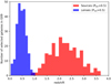 |
Fig. 3. Comparison between the redshift distributions of the lenses (blue) and sources (red) selected by SHALOS with Ptot > 0.5. |
In Table 3 there is a summary of the number of galaxies initially in the H-ATLAS catalogues and the number of identified SLGs at different Ptot values for each of the four fields considered. We also show the number of selected sources (with SDSS counterparts, estimated optical redshifts, and not flagged as stars) at high redshift (z > 0.8) with reliable flux density measurements (at least 3σ photometric estimations at 350 and 500 μm).
Summary of the SHALOS results statistics.
There are already several interesting conclusions that can be extracted from these results: i) Only ∼7% of the initial H-ATLAS sources have an optical counterpart and are considered reliable high redshift sources, z > 0.8 with our current selection criteria; ii) The results are homogeneous among the different fields and have minimal percentage variations; iii) More than half of the high redshift selected sources have a close low-z optical counterpart and, therefore, they have a non-negligible associated probability, Ptot > 0.1, of being a SLG. This result is in agreement with the strong magnification bias signal measured by González-Nuevo et al. (2014, 2017), which implies that many of the H-ATLAS high-z sources are slightly enhanced by weak gravitational lensing; iv) The probability of a stronger gravitational effect is boosted by increasing the Ptot limit due to the luminosity percentile observable effect. The number of candidates with Ptot > 0.5 is greater than 1000, confirming the HALOS predictions (González-Nuevo et al. 2012) that with more complex selection procedures it is possible to reach such numbers; v) Finally, the most probable candidates, Ptot > 0.7, correspond to 447 (or 0.19%) that it is ∼5 times the 80 H-ATLAS candidates found with flux density above 100 mJy at 500 μm (Negrello et al. 2017). Taking into account that Negrello et al. (2017) found 30 SLG candidates in the SGP field, this factor increases to 447/50 ∼ 9 for the common area.
As a check of our results, we compared SHALOS SLG candidates with those found in Negrello et al. (2017). In the common NGP and GAMA fields, Negrello et al. (2017) found 50 SLG candidates, but only 32 are identified in SHALOS. We excluded the other 18 objects either because they have no estimated optical redshift (needed by SHALOS) or because, in the case of three, they are flagged as stars, and we are not interested in such objects. We would like to remark that the fact that we found three potential optical counterparts flagged as stars in the Negrello et al. (2017) list of candidates only indicates that the lens galaxy was detected by SDSS or it was not correctly matched to the background sources with the LR technique. The Negrello et al. (2017) identification method is based only on galaxy source photometry and therefore is completely independent of any potential optical counterpart.
On the one hand, following the Negrello et al. (2017) selection criteria, we selected those SHALOS SLG candidates with a flux density at 500 μm greater than 100 mJy and redshift greater than 0.1, to avoid very local objects. By applying such redshift and flux density selection in SHALOS, we obtained a list of 42 objects with Ptot > 0.1, again with the common 32 SLG candidates. There are new 10 objects that are in SHALOS and not in Negrello et al. (2017). Six of these have Ptot < 0.5, i.e. a very low probability of being actual SLGs; 3 are identified as blazars (see Table 1 in Negrello et al. 2017, i.e. they have estimated photometric redshifts much higher than the potential lenses and therefore they obtain a high Ptot); and 1 is a local extended source (NGC 5705) so that its SPIRE photometry is not reliable for the possible, if there is any, background source.
Therefore, not only is the SHALOS method as effective as the Negrello et al. (2017) approach for S500 μm > 100 mJy (for lensing systems in which the lens is detected in SDSS), but it is also able to extend the identification methodology at lower flux density limits.
5. Validation by induction
Only a follow-up campaign using top instruments with high resolution and sensitivity could establish the overall performance of the proposed methodology by studying each individual SLG candidate one by one. However, even obtaining observational time in such facilities, it will take months, if not years, to built a database large enough to derive some meaningful statistics.
For this reason, we propose an alternative and complementary approach to validate the SHALOS methodology: validation by induction. In this section we assume that all the lensing event candidates are confirmed SLGs and study some of their statistical properties. Then, we can compare such properties with previous results or theoretical expectations to check if they are in agreement. If this is the case, we can conclude that the SHALOS provided list is consistent with being mainly composed by SLGs. Therefore, we can use the SHALOS list to obtain additional valuable statistical information about these kinds of events thanks to its less restrictive limits.
5.1. Amplification factors
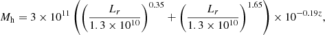
The first statistical property calculated is a tentative amplification factor, μ, produced by the gravitational lensing effect: there is enough information in the SHALOS list to derive an approximate μ for each of the event candidates. The SHALOS purpose is to identify SLGs and therefore the selected candidates are expected to have amplification factors at least of > 1.2 − 1.5. Taking into account the relative uncertainty in the estimation, if the results had shown that statistically all the amplification factors are ∼1 then this would have been a serious indication of the failure of the methodology.
Following mainly the same procedure as in González-Nuevo et al. (2014), we estimated for each lens the stellar mass, M⋆, from the r-band luminosity, Lr. We considered two different scenarios: first, the gravitational lensing effect is produced mainly by the galactic halo surrounding the lens galaxy; second, lens galaxies are typically the central galaxy of a group or cluster of galaxies as indicated by the conclusions obtained by González-Nuevo et al. (2014) and González-Nuevo et al. (2017). In this case we thus estimated a group or cluster of galaxies halo mass.
In the first case, we considered a singular isothermal sphere (SIS) mass density profile and we derived the galactic halo mass, Mh, directly from the r-band luminosity (Shankar et al. 2006; Bernardi et al. 2003) as follows:
with Mh and Lr in M⊙ and L⊙, respectively.
For the second scenario, we considered a Navarro–Frank–White mass density profile (Navarro et al. 1996). We calculated the stellar mass using a modified version of the luminosity-stellar mass relationship (Bernardi et al. 2003, 2010), i.e.

with M⋆ and Lr in M⊙ and L⊙, respectively. Then we estimated the cluster halo mass by applying the stellar to halo mass relationship derived by Moster et al. (2010).
Finally, the amplification factors, i.e. total amplification, for both scenario were estimated following the traditional gravitational lensing framework (see for example Schneider et al. 2006), taking into account the derived halo masses and the source and lens redshifts. We used the concentration formula derived by Prada et al. (2012).
The results, for all the different areas together, are shown in Fig. 4 for two different Ptot cuts. Even with these tentative estimations about the amplification factors, these results are encouraging, as stated at the beginning of this section. The mean (median) values of the SHALOS list for Ptot > 0.5 is 1.90 (1.26) for the galactic halo case and 2.51 (1.39) for the cluster case. For a more conservative cut, with Ptot > 0.7, the obtained amplification factors are on average bigger: 2.28 (1.33) for the galactic halo and 3.12 (1.47) for the cluster case. With these estimated amplification factors, the fraction of SHALOS candidates with Ptot > 0.5 that have μ > 2 are 17.2% and 25.8% for the galactic and cluster scenarios, respectively. These percentages increase to 24.3% and 31.5%, respectively, for the Ptot > 0.7 cut.
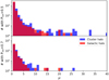 |
Fig. 4. Tentative amplification factors derived assuming a galactic and cluster halo masses (see text for more details). |
5.2. Auto-correlation function
The number of SHALOS candidates is large enough to measure their two-point correlation function. If the SHALOS candidates were simply random associations their correlation function would have been negligible or noise dominated; they are too sparse to be affected by the clustering properties of the background sample. At maximum they could have resembled the correlation of the SMGs or background sample. On the contrary, if they are real SLGs their correlation function would be in agreement with that expected from a foreground sample with the lens derived masses.
To check these possibilities, we estimated the two points correlation function of the SHALOS candidates using the Landy & Szalay (1993) estimator,
where DD, DR, and RR are the normalized unique pairs of galaxies, data-random pairs, and random-random pairs, respectively.
The measured correlation functions for Ptot > 0.5 & 0.7 are shown in Fig. 5. Although the uncertainties are significant, the SHALOS candidates have a non-zero or noise dominated correlation function. This result immediately discards the random association hypothesis. Moreover, the SHALOS candidates correlation is stronger than those measured by González-Nuevo et al. (2017) for the Herschel SMGs at z > 1.2 (black diamonds) or those found in the more recent Amvrosiadis et al. (2019). These galaxies are the same galaxies that constitute our background sample. Therefore, it is confirmed that there is something special about the SHALOS selected background galaxies.
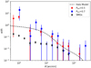 |
Fig. 5. Auto-correlation of SHALOS SLGs with Ptot > 0.5 & 0.7 compared with the theoretical estimation using the González-Nuevo et al. (2017) observed cross-correlation parameters. The González-Nuevo et al. (2017) measured auto-correlation of the H-ATLAS high-z sources (black circles) is also shown as a comparison. |
Finally, we calculated, for comparison, the correlation function expected for a sample of lenses with the observed redshift distribution (blue histogram in Fig. 3) and the mass and halo occupation distribution properties derived by González-Nuevo et al. (2017) for the foreground lenses sample: minimum halo mass of ∼1.3 × 10¹³ M⊙, a pivotal mass to have at least one satellite galaxy of ∼3.7 × 10¹⁴ M⊙ and the slope of the number of satellites, ∼2. These values were measured by studying the cross-correlation signal between a foreground sample of GAMA galaxies with spectroscopic redshifts in the range 0.2 < z < 0.8, and a background sample of H-ATLAS galaxies with photometric redshifts ≳1.2. By using the same halo model formalism of González-Nuevo et al. (2017), mainly based on Cooray & Sheth (2002), we derived the dashed black line that corresponds to the correlation properties of the foreground lenses. This theoretical estimation is in good agreement with our measured correlation function.
Therefore, we can conclude that the angular correlation properties of the SHALOS selected candidates closely resemble those expected for the sample of foreground lenses and not to the background parent population sources. It is not a direct validation of the gravitational lensing nature of the SHALOS candidates but it is an additional statistical property that agrees with the expectations.
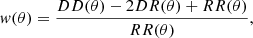
5.3. Source number counts
The integral source number counts at 500 μm of the SHALOS candidates, combining the results for all the four H-ATLAS fields, are shown in Fig. 6. We applied two different Ptot cuts to check the number counts dependence on the associated probability. Above 100 mJy, we can compare the SHALOS source number counts with those derived with the most simple but robust identification methodology by Negrello et al. (2017) (grey diamonds) using the same H-ATLAS catalogues. Nayyeri et al. (2016) obtained almost identical source number counts with the same methodology but for the HeLMS+HerS survey (not shown in the figure).
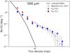 |
Fig. 6. Integrated source number counts at 500 μm of the SHALOS candidates with Ptot > 0.5 & 0.7 (red circles and blue squares, respectively). These counts are compared with the integrated number counts of candidate lensed galaxies derived by Negrello et al. (2017) from all the H-ATLAS fields (grey diamonds). The error bars correspond to the 95% confidence interval. We also show the model source number counts for the unlensed SMGs (black line; Lapi et al. 2011; Cai et al. 2013). |
In general, there is good agreement between both sets of lensed candidates source number counts. However, the fact that Negrello et al. (2017) identified additional SLGs without optical counterparts explains the slightly higher source number counts around 100 mJy.
On the other hand, the SHALOS methodology allows us to extend the measurement of the source number counts down to 50 mJy. It is at these fainter flux densities that the effect of the different Ptot cuts is more relevant. A lower probability cut tend to select more lensed candidates but mainly at fainter flux limits, S500 μm < 100 mJy. Although we are reaching flux densities that start to be dominated by the unlensed SMGs, the SHALOS methodology seems to be effective to discriminate between the lensed or unlensed nature of the considered SMGs, at least for the Ptot > 0.7 cut, as also indicated by the results of Sect. 5.2.
We can conclude that the SHALOS candidates source number counts at 500 μm above 100 mJy are in good agreement with previous estimations, where many of the candidates were confirmed by follow-up observations. Therefore, both methodologies are equivalent at such flux densities. The advantage of the SHALOS approach is that it is able to extend the identification of reliable SLG candidates down to lower flux densities, ∼50 mJy.
6. Conclusions
We propose a new methodology for the identification of objects with particular properties by cross-matching various catalogues based on the similarity of probability distribution (the BC) associated with different observables. This new approach is more simple, objective, and flexible than other traditional approaches to the problem, such as the LR or the Bayes factor.
As a practical application, in this work we have focussed on the identification of SMGs in the Herschel-ATLAS whose flux density was strongly amplified by the gravitational lensing effect produced by SDSS galaxies at z < 0.8, acting as the lenses. In particular, we derived the total estimated probability, Ptot, of being lensed based on four observables: the angular separation, the bolometric luminosity percentile compared with SMGs at similar redshift, the redshift difference, and the ratio of the optical to the submillimetre emissions. The results indicate, as also confirmed by a PCA analysis, that the first two are the most discriminant for the identification task. The other two help to confirm that the cross-matched pairs are not the same galaxy, but two galaxies at different redshfits.
The SHALOS method identified 1451 SLG candidates with Ptot > 0.5, which correspond to 0.61% of the H-ATLAS sources. This number decreases to 447 (or 0.19%) with a more conservative Ptot > 0.7, that it is still ∼5 times the number of SLGs found by Negrello et al. (2017). When comparing both SLGs lists, the SHALOS method was able to identify 32 of the 50 SLGs with flux density at 500 μm greater than ∼100 mJy. The remaining 18 SLG candidates were excluded by SHALOS because of the lack of an optical redshift estimation or because they were flagged as stars. On the contrary, the SHALOS method found 4 SLG candidates with Ptot > 0.5 not in Negrello et al. (2017): 3 are identified blazars (see Table 1 in Negrello et al. 2017) and 1 is a local extended galaxy (NGC 5705).
Finally, we studied some characteristic statistical properties of the SHALOS SLG candidates as the estimated amplifications factors: the two-point correlation function and the source number counts. For Ptot > 0.7, the tentative amplification factors were found to have mean(median) of 2.28 (1.33) for a galactic mass halo and 3.12 (1.47) for a cluster mass halo. The number of SHALOS candidates with Ptot > 0.7 and μ > 2 are 24.3% and 31.5% for the galactic and cluster scenarios recpectively. Moreover, the SHALOS candidates have a non-zero correlation function that is stronger than that measured for the background SMG sample in González-Nuevo et al. (2017). It is in agreement with the correlation function expected for the foreground lenses (massive elliptical galaxies or even group of galaxies as anticipated by González-Nuevo et al. 2014 and confirmed by González-Nuevo et al. 2017). The SHALOS candidates source number counts at 500 μm above 100 mJy are in good agreement with previous results confirming that both methodologies are equivalent. However, the SHALOS method allows us to reach much lower flux densities, i.e. ∼50 mJy. At such faint flux densities, the total source number counts start to be dominated by unlensed SMGs, but the derived source number counts seems to indicate the effectiveness of the SHALOS methodology even in distinguishing between lensed or unlensed SMGs
Acknowledgments
We would like to thank Dr. Mattia Negrello for his exhaustive and valuable comments that helped us to improve the clarity a robustness of the present work. JGN, LB, FA, LT, and SLSG acknowledge financial support from the I+D 2015 project AYA2015-65887-P (MINECO, FEDER) and the PGC 2018 project PGC2018-101948-B-I00 (MINECO, FEDER). JGN acknowledges financial from the Spanish MINECO for a “Ramon y Cajal” fellowship (RYC-2013-13256). DH, FA, and LT acknowledge financial support from the I+D 2015 project AYA2015-64508-P (MINECO, FEDER). DH also acknowledges partial financial support from the RADIOFOREGROUNDS project, funded by the European Comission’s H2020 Research Infrastructures under the Grant Agreement 687312. JDCJ acknowledge financial support from the I+D 2017 project AYA2017-89121-P and support from the European Union’s Horizon 2020 research and innovation programme under the H2020-INFRAIA-2018-2020 grant agreement No 210489629. The Herschel-ATLAS is a project with Herschel, which is an ESA space observatory with science instruments provided by European-led Principal Investigator consortia and with important participation from NASA. The H-ATLAS website is http://www.h-atlas.org/. This research has made use of TopCat (Taylor et al. 2005), and the python packages ipython (Pérez & Granger 2007), matplotlib (Hunter 2007), Scipy (Jones et al. 2001), and Astropy, a community-developed core Python package for Astronomy (Astropy Collaboration 2013).
References
- Abazajian, K. N., Adelman-McCarthy, J. K., Agüeros, M. A., et al. 2009, ApJS, 182, 543 [NASA ADS] [CrossRef] [Google Scholar]
- Amvrosiadis, A., Valiante, E., Gonzalez-Nuevo, J., et al. 2019, MNRAS, 483, 4649 [CrossRef] [Google Scholar]
- Astropy Collaboration (Robitaille, T. P., et al.) 2013, A&A, 558, A33 [NASA ADS] [CrossRef] [EDP Sciences] [Google Scholar]
- Berger, J. O., & Pericchi, L. R. 1996, J. Am. Stat. Assoc., 91, 109 [CrossRef] [Google Scholar]
- Bernardi, M., Sheth, R. K., Annis, J., et al. 2003, AJ, 125, 1849 [NASA ADS] [CrossRef] [Google Scholar]
- Bernardi, M., Shankar, F., Hyde, J. B., et al. 2010, MNRAS, 404, 2087 [NASA ADS] [Google Scholar]
- Bhattacharyya, A. 1943, Bull. Calcutta Math. Soc., 35, 99 [Google Scholar]
- Blain, A. W. 1996, MNRAS, 283, 1340 [NASA ADS] [CrossRef] [Google Scholar]
- Blain, A. W. 1999, MNRAS, 304, 669 [NASA ADS] [CrossRef] [Google Scholar]
- Bonavera, L., González-Nuevo, J., Suárez Gómez, S. L., et al. 2019, JCAP, submitted [arXiv:1902.03624] [Google Scholar]
- Bourne, N., Maddox, S. J., Dunne, L., et al. 2014, MNRAS, 444, 1884 [CrossRef] [Google Scholar]
- Bourne, N., Dunne, L., Maddox, S. J., et al. 2016, MNRAS, 462, 1714 [NASA ADS] [CrossRef] [Google Scholar]
- Budavári, T. 2011, ApJ, 736, 155 [NASA ADS] [CrossRef] [Google Scholar]
- Budavári, T., & Szalay, A. S. 2008, ApJ, 679, 301 [NASA ADS] [CrossRef] [PubMed] [Google Scholar]
- Bussmann, R. S., Gurwell, M. A., Fu, H., et al. 2012, ApJ, 756, 134 [NASA ADS] [CrossRef] [Google Scholar]
- Bussmann, R. S., Pérez-Fournon, I., Amber, S., et al. 2013, ApJ, 779, 25 [NASA ADS] [CrossRef] [Google Scholar]
- Cañameras, R., Nesvadba, N. P. H., Guery, D., et al. 2015, A&A, 581, A105 [NASA ADS] [CrossRef] [EDP Sciences] [Google Scholar]
- Cai, Z.-Y., Lapi, A., Xia, J.-Q., et al. 2013, ApJ, 768, 21 [NASA ADS] [CrossRef] [Google Scholar]
- Calanog, J. A., Fu, H., Cooray, A., et al. 2014, ApJ, 797, 138 [NASA ADS] [CrossRef] [Google Scholar]
- Carlstrom, J. E., Ade, P. A. R., Aird, K. A., et al. 2011, PASP, 123, 568 [NASA ADS] [CrossRef] [Google Scholar]
- Choi, E., & Lee, C. 2003, Pattern Recognit., 36, 1703 [CrossRef] [Google Scholar]
- Cooray, A., & Sheth, R. 2002, Phys. Rep., 372, 1 [NASA ADS] [CrossRef] [Google Scholar]
- Coppin, K., Chapin, E. L., Mortier, A. M. J., et al. 2006, MNRAS, 372, 1621 [NASA ADS] [CrossRef] [Google Scholar]
- Eales, S., Dunne, L., Clements, D., et al. 2010, PASP, 122, 499 [NASA ADS] [CrossRef] [Google Scholar]
- Fleuren, S., Sutherland, W., Dunne, L., et al. 2012, MNRAS, 423, 2407 [NASA ADS] [CrossRef] [Google Scholar]
- Fu, H., Jullo, E., Cooray, A., et al. 2012, ApJ, 753, 134 [NASA ADS] [CrossRef] [Google Scholar]
- Furlanetto, C., Dye, S., Bourne, N., et al. 2018, MNRAS, 476, 961 [NASA ADS] [Google Scholar]
- González-Nuevo, J., Lapi, A., Fleuren, S., et al. 2012, ApJ, 749, 65 [NASA ADS] [CrossRef] [Google Scholar]
- González-Nuevo, J., Lapi, A., Negrello, M., et al. 2014, MNRAS, 442, 2680 [NASA ADS] [CrossRef] [Google Scholar]
- González-Nuevo, J., Lapi, A., Bonavera, L., et al. 2017, JCAP, 10, 024 [CrossRef] [Google Scholar]
- Granato, G. L., De Zotti, G., Silva, L., Bressan, A., & Danese, L. 2004, ApJ, 600, 580 [Google Scholar]
- Griffin, M. J., Abergel, A., Abreu, A., et al. 2010, A&A, 518, L3 [Google Scholar]
- Harrington, K. C., Yun, M. S., Cybulski, R., et al. 2016, MNRAS, 458, 4383 [NASA ADS] [CrossRef] [Google Scholar]
- Hunter, J. D. 2007, Comput. Sci. Eng., 9, 90 [NASA ADS] [CrossRef] [Google Scholar]
- Ibar, E., Ivison, R. J., Cava, A., et al. 2010, MNRAS, 409, 38 [NASA ADS] [CrossRef] [Google Scholar]
- Ivison, R. J., Swinbank, A. M., Swinyard, B., et al. 2010, A&A, 518, L35 [NASA ADS] [CrossRef] [EDP Sciences] [Google Scholar]
- Ivison, R. J., Lewis, A. J. R., Weiss, A., et al. 2016, ApJ, 832, 78 [NASA ADS] [CrossRef] [Google Scholar]
- Jones, E., Oliphant, T., Peterson, P., et al. 2001, SciPy: Open source scientific tools for Python [Google Scholar]
- Landy, S. D., & Szalay, A. S. 1993, ApJ, 412, 64 [NASA ADS] [CrossRef] [Google Scholar]
- Lapi, A., González-Nuevo, J., Fan, L., et al. 2011, ApJ, 742, 24 [NASA ADS] [CrossRef] [Google Scholar]
- Lapi, A., Negrello, M., González-Nuevo, J., et al. 2012, ApJ, 755, 46 [NASA ADS] [CrossRef] [Google Scholar]
- Maddox, S. J., Valiante, E., Cigan, P., et al. 2018, ApJS, 236, 30 [NASA ADS] [CrossRef] [Google Scholar]
- Messias, H., Dye, S., Nagar, N., et al. 2014, A&A, 568, A92 [NASA ADS] [CrossRef] [EDP Sciences] [Google Scholar]
- Moster, B. P., Somerville, R. S., Maulbetsch, C., et al. 2010, ApJ, 710, 903 [NASA ADS] [CrossRef] [Google Scholar]
- Navarro, J. F., Frenk, C. S., & White, S. D. M. 1996, ApJ, 462, 563 [NASA ADS] [CrossRef] [Google Scholar]
- Nayyeri, H., Keele, M., Cooray, A., et al. 2016, ApJ, 823, 17 [NASA ADS] [CrossRef] [Google Scholar]
- Negrello, M., Perrotta, F., González-Nuevo, J., et al. 2007, MNRAS, 377, 1557 [NASA ADS] [CrossRef] [Google Scholar]
- Negrello, M., Hopwood, R., De Zotti, G., et al. 2010, Science, 330, 800 [NASA ADS] [CrossRef] [Google Scholar]
- Negrello, M., Hopwood, R., Dye, S., et al. 2014, MNRAS, 440, 1999 [NASA ADS] [CrossRef] [Google Scholar]
- Negrello, M., Amber, S., Amvrosiadis, A., et al. 2017, MNRAS, 465, 3558 [NASA ADS] [CrossRef] [Google Scholar]
- Odewahn, S. C., Stockwell, E. B., Pennington, R. L., Humphreys, R. M., & Zumach, W. A. 1992, AJ, 103, 318 [NASA ADS] [CrossRef] [Google Scholar]
- Oliver, S. J., Bock, J., Altieri, B., et al. 2012, MNRAS, 424, 1614 [NASA ADS] [CrossRef] [EDP Sciences] [Google Scholar]
- Pascale, E., Auld, R., Dariush, A., et al. 2011, MNRAS, 415, 911 [NASA ADS] [CrossRef] [Google Scholar]
- Pearson, E. A., Eales, S., Dunne, L., et al. 2013, MNRAS, 435, 2753 [NASA ADS] [CrossRef] [Google Scholar]
- Pérez, F., & Granger, B. E. 2007, Comput. Sci. Eng., 9, 21 [Google Scholar]
- Pilbratt, G. L., Riedinger, J. R., Passvogel, T., et al. 2010, A&A, 518, L1 [CrossRef] [EDP Sciences] [Google Scholar]
- Poglitsch, A., Waelkens, C., Geis, N., et al. 2010, A&A, 518, L2 [NASA ADS] [CrossRef] [EDP Sciences] [Google Scholar]
- Prada, F., Klypin, A. A., Cuesta, A. J., Betancort-Rijo, J. E., & Primack, J. 2012, MNRAS, 423, 3018 [NASA ADS] [CrossRef] [Google Scholar]
- Ray, S. 1989, Pattern Recognit. Lett., 9, 315 [CrossRef] [Google Scholar]
- Richter, G. A. 1975, Astron. Nachr., 296, 65 [NASA ADS] [CrossRef] [Google Scholar]
- Rigby, E. E., Maddox, S. J., Dunne, L., et al. 2011, MNRAS, 415, 2336 [NASA ADS] [CrossRef] [Google Scholar]
- Schneider, P., Kochanek, C., & Wambsganss, J. 2006, Gravitational Lensing: Strong, Weak and Micro (Springer) [Google Scholar]
- Shankar, F., Lapi, A., Salucci, P., De Zotti, G., & Danese, L. 2006, ApJ, 643, 14 [NASA ADS] [CrossRef] [MathSciNet] [Google Scholar]
- Smith, D. J. B., Dunne, L., Maddox, S. J., et al. 2011, MNRAS, 416, 857 [NASA ADS] [CrossRef] [Google Scholar]
- Smith, D. J. B., Dunne, L., da Cunha, E., et al. 2012, MNRAS, 427, 703 [NASA ADS] [CrossRef] [Google Scholar]
- Smith, M. W. L., Ibar, E., Maddox, S. J., et al. 2017, ApJS, 233, 26 [NASA ADS] [CrossRef] [Google Scholar]
- Spilker, J. S., Marrone, D. P., Aravena, M., et al. 2016, ApJ, 826, 112 [NASA ADS] [CrossRef] [Google Scholar]
- Storrie-Lombardi, M. C., Lahav, O., Sodre, Jr., L., & Storrie-Lombardi, L. J. 1992, MNRAS, 259, 8P [NASA ADS] [CrossRef] [Google Scholar]
- Sutherland, W., & Saunders, W. 1992, MNRAS, 259, 413 [NASA ADS] [CrossRef] [Google Scholar]
- Swinbank, A. M., Smail, I., Longmore, S., et al. 2010, Nature, 464, 733 [Google Scholar]
- Taylor, M. B. 2005, in Astronomical Data Analysis Software and Systems XIV, eds. P. Shopbell, M. Britton, & R. Ebert, ASP Conf. Ser., 347, 29 [Google Scholar]
- Valiante, E., Smith, M. W. L., Eales, S., et al. 2016, MNRAS, 462, 3146 [NASA ADS] [CrossRef] [Google Scholar]
- Vieira, J. D., Marrone, D. P., Chapman, S. C., et al. 2013, Nature, 495, 344 [NASA ADS] [CrossRef] [Google Scholar]
- Viero, M. P., Asboth, V., Roseboom, I. G., et al. 2014, ApJS, 210, 22 [NASA ADS] [CrossRef] [Google Scholar]
- Wardlow, J. L., Cooray, A., De Bernardis, F., et al. 2013, ApJ, 762, 59 [NASA ADS] [CrossRef] [Google Scholar]
All Tables
Loadings of PCA for each of the considered observables (BCpos, (1 − BCr), (1 − BCz), Lperc), and their correspondent influence on each of the components.
Relevancy of PCA components considering standard deviation, proportion of explained variance and the cumulative proportion of variance.
All Figures
|
Fig. 1. Comparison for the GAMA12 field of the variation of the number of sources with the different probabilities associated with the observables considered in this work. Similar results are obtained for the other fields. The total probability is shown as a thick black line while the estimated probability of random pairs is shown as a grey line. |
| In the text | |
|
Fig. 2. Comparison between Ptot and the likelihood reliability. |
| In the text | |
|
Fig. 3. Comparison between the redshift distributions of the lenses (blue) and sources (red) selected by SHALOS with Ptot > 0.5. |
| In the text | |
|
Fig. 4. Tentative amplification factors derived assuming a galactic and cluster halo masses (see text for more details). |
| In the text | |
|
Fig. 5. Auto-correlation of SHALOS SLGs with Ptot > 0.5 & 0.7 compared with the theoretical estimation using the González-Nuevo et al. (2017) observed cross-correlation parameters. The González-Nuevo et al. (2017) measured auto-correlation of the H-ATLAS high-z sources (black circles) is also shown as a comparison. |
| In the text | |
|
Fig. 6. Integrated source number counts at 500 μm of the SHALOS candidates with Ptot > 0.5 & 0.7 (red circles and blue squares, respectively). These counts are compared with the integrated number counts of candidate lensed galaxies derived by Negrello et al. (2017) from all the H-ATLAS fields (grey diamonds). The error bars correspond to the 95% confidence interval. We also show the model source number counts for the unlensed SMGs (black line; Lapi et al. 2011; Cai et al. 2013). |
| In the text | |
Current usage metrics show cumulative count of Article Views (full-text article views including HTML views, PDF and ePub downloads, according to the available data) and Abstracts Views on Vision4Press platform.
Data correspond to usage on the plateform after 2015. The current usage metrics is available 48-96 hours after online publication and is updated daily on week days.
Initial download of the metrics may take a while.