| Issue |
A&A
Volume 627, July 2019
|
|
|---|---|---|
| Article Number | A118 | |
| Number of page(s) | 17 | |
| Section | The Sun | |
| DOI | https://doi.org/10.1051/0004-6361/201935233 | |
| Published online | 10 July 2019 | |
Temporal evolution and correlations of optical activity indicators measured in Sun-as-a-star observations⋆
1
INAF – Osservatorio Astronomico di Palermo, Piazza del Parlamento 1, 90134 Palermo, Italy
e-mail: This email address is being protected from spambots. You need JavaScript enabled to view it.
2
Harvard-Smithsonian Center for Astrophysics, 60 Garden Street, Cambridge, MA 02138, USA
3
Observatoire Astronomique de l’Université de Genève, 51 Chemin des Maillettes, 1290 Sauverny, Switzerland
4
SUPA, School of Physics and Astronomy, University of St Andrews, North Haugh, St Andrews KY16 9SS, UK
5
Centre for Exoplanet Science, University of St Andrews, St Andrews, UK
6
INAF – Osservatorio Astrofisico di Catania, Via S. Sofia 78, 95123 Catania, Italy
7
Astrophysics Group, Cavendish Laboratory, University of Cambridge, J.J. Thomson Avenue, Cambridge CB3 0HE, UK
8
INAF – Osservatorio Astrofisico di Torino, Via Osservatorio 20, 10025 Pino Torinese, Italy
9
SUPA, Institute for Astronomy, Royal Observatory, University of Edinburgh, Blackford Hill, Edinburgh EH9 3HJ, UK
10
Centre for Exoplanet Science, University of Edinburgh, Edinburgh, UK
11
Department of Physics, Harvard University, 17 Oxford Street, Cambridge, MA 02138, USA
12
INAF – Fundación Galileo Galilei, Rambla José Ana Fernandez Pérez 7, 38712 Breña Baja, Tenerife, Spain
13
Astrophysics Research Centre, School of Mathematics and Physics, Queen’s University Belfast, University Road, Belfast BT7 1NN, UK
14
INAF – Osservatorio Astronomico di Cagliari, Via della Scienza 5, 09047 Selargius, Italy
15
INAF – Osservatorio Astronomico di Padova, Vicolo dell’Osservatorio 5, 35122 Padova, Italy
16
Dipartimento di Fisica e Astronomia “Galileo Galilei”, Università di Padova, Vicolo dell’Osservatorio 3, 35122 Padova, Italy
17
INAF – Osservatorio Astronomico di Brera, Via E. Bianchi 46, 23807 Merate LC, Italy
Received:
8
February
2019
Accepted:
6
June
2019
Abstract
Context. Understanding stellar activity in solar-type stars is crucial for the physics of stellar atmospheres as well as for ongoing exoplanet programmes.
Aims. We aim to test how well we understand stellar activity using our own star, the Sun, as a test case.
Methods. We performed a detailed study of the main optical activity indicators (Ca II H & K, Balmer lines, Na I D1 D2, and He I D3) measured for the Sun using the data provided by the HARPS-N solar-telescope feed at the Telescopio Nazionale Galileo. We made use of periodogram analyses to study solar rotation, and we used the pool variance technique to study the temporal evolution of active regions. The correlations between the different activity indicators as well as the correlations between activity indexes and the derived parameters from the cross-correlation technique are analysed. We also study the temporal evolution of these correlations and their possible relationship with indicators of inhomogeneities in the solar photosphere like sunspot number or radio flux values.
Results. The value of the solar rotation period is found in all the activity indicators, with the only exception being Hδ. The derived values vary from 26.29 days (Hγ line) to 31.23 days (He I). From an analysis of sliding periodograms we find that in most of the activity indicators the spectral power is split into several “bands” of periods around 26 and 30 days. They might be explained by the migration of active regions between the equator and a latitude of ∼30°, spot evolution, or a combination of both effects. A typical lifetime of active regions of approximately ten rotation periods is inferred from the pooled variance diagrams, which is in agreement with previous works. We find that Hα, Hβ, Hγ, Hϵ, and He I show a significant correlation with the S index. Significant correlations between the contrast, bisector span, and the heliocentric radial velocity with the activity indexes are also found. We show that the full width at half maximum, the bisector, and the disc-integrated magnetic field correlate with the radial velocity variations. The correlation of the S index and Hα changes with time, increasing with larger sun spot numbers and solar irradiance. A similar tendency with the S index and radial velocity correlation is also present in the data.
Conclusions. Our results are consistent with a scenario in which higher activity favours the correlation between the S index and the Hα activity indicators and between the S index and radial velocity variations.
Key words: Sun: activity / Sun: chromosphere / Sun: rotation / techniques: spectroscopic
Table A.1 is only available at the CDS via anonymous ftp to cdsarc.u-strasbg.fr (130.79.128.5) or via http://cdsarc.u-strasbg.fr/viz-bin/qcat?J/A+A/627/A118
NASA Sagan Fellow.
CHEOPS Fellow, SNSF NCCR-PlanetS.
© ESO 2019
1. Introduction
Our own star, the Sun, constitutes a benchmark in the study of stellar magnetic activity. Unlike other stars, the solar surface can be resolved, and direct information about the size, contrast, or the location of surface inhomogeneities can be obtained.
Understanding stellar activity is crucial for the detection of small, rocky, potentially habitable planets around low-mass stars (e.g. Fischer et al. 2016). The detection of Earth-twins via the radial velocity technique requires a radial velocity precision of the order of 10 cm s−1 which is an order of magnitude lower than the radial velocity variations induced by the presence of inhomogeneities (cool spots, hot faculae, and plages) in the stellar surface, typically between 1 and 200 ms−1 with timescales of 2−50 days in solar-type stars (e.g. Hatzes 2016). The apparent radial velocity variations of the Sun-as-a-star are between 1 and 20 ms−1 over timescales from days to years (Meunier et al. 2010a; Dumusque et al. 2015; Haywood et al. 2016; Lanza et al. 2016). Variations as large as 200 ms−1 are localised into spotted and facular regions (Meunier et al. 2010a), but they are much reduced when averaged over the whole solar disc.
With the aim of a better understanding of stellar signals the small solar telescope at the Telescopio Nazionale Galileo (TNG) is able to obtain precise full-disc radial velocity measurements of the Sun using the HARPS-N spectrograph (Dumusque et al. 2015; Phillips et al. 2016; Milbourne et al. 2019; Cameron et al. 2019). The approach is to observe the Sun-as-a-star, allowing us to directly correlate any change in the observed surface inhomogeneities with variations in the full-disc radial velocity.
The HARPS-N solar data offer an unique opportunity to acquire a deeper understanding of how solar (and by extension stellar) activity produces apparent radial velocity variations. Therefore, in this paper we present a detailed analysis of the main optical activity indicators (Ca II H & K, Balmer lines, Na I D1 D2, and He I D3) measured during the first three years of the solar telescope operations.
This paper is organised as follows. Section 2 describes the observations. The periodogram analysis and the correlations between different activity indicators is presented in Sect. 3. The results are discussed at length in Sect. 4. Our conclusions follow in Sect. 5.
2. Observations
To date, the Sun has been observed for a period of 1049 days (i.e. ∼2.9 yr) from Barycentric Julian Date BJD = 2457218 (July 14, 2015) to BJD = 2458267 (May 29, 2018), corresponding to the late phase of the 24th solar cycle. A total of 48335 HARPS-N observations were collected during this period. The median number of observations per day is 45, although in some days the number of observations can be as high as 80.
HARPS-N spectra cover the wavelength range 383−693 nm with a resolving power of R ∼ 115 000. Data were reduced using the latest version of the Data Reduction Software (DRS V3.7, Lovis & Pepe 2007) which implements the typical corrections involved in échelle spectra reduction, including bias level, flat-fielding, order extraction, wavelength calibration, and merging of individual orders. Radial velocities (RVs) are computed by cross-correlating the spectra of the target star with an optimised binary mask (Baranne et al. 1996; Pepe et al. 2002). For the Sun the G2 mask was used. The HARPS-N DRS also provides several CCF asymmetry diagnostics, such as the CCF width (FWHM), the bisector span (BIS), and the CCF contrast. Typical values of the signal-to-noise ratio (S/N) around 5500 Å are ∼380, although in the period between BJD 2458060 and 2458160 the achieved S/N decreases due to a damaged optical fibre and typical values are around 130.
Activity indexes in the main optical indicators, Ca II H & K, Balmer lines (from Hα to Hϵ), Na I D1 D2, and He I D3 were computed. Our definition of the bandpasses for the Ca II H & K activity S index is made following Henry et al. (1996), using a triangular filter in the core of the lines. We note that this is the only index for which a triangular shape is used. S index values were corrected for the presence of ghosts and transformed to the Mount Wilson scale using the relationship provided by Lovis et al. (2011). We note that the use of R′HK is not needed for the purpose of this work. Our scope is to compare different activity indicators and analogous quantities to the R′HK have not been defined for other activity-sensitive lines. For the Hα, He I, and Na I indexes the definitions by Gomes da Silva et al. (2011) were followed. For the rest of the Balmer lines the prescriptions given by West & Hawley (2008) were used. In some cases, small changes in the width of the continuum passbands were introduced. Our bandpasses are summarised in Table 1. Fluxes were measured using the IRAF1 task SBANDS. Before measuring the fluxes, each individual spectrum was corrected for its corresponding radial velocity (see below) using the IRAF task DOPCOR. Uncertainties in the activity indexes are computed from the uncertainties in each bandpass which are computed as:
Bandpasses for the activity indexes considered in this work.
![Mathematical equation: $$ \begin{aligned} \Delta F = \frac{1}{\sqrt{n}} \left[\frac{F}{S/N}\right] \end{aligned} $$](/articles/aa/full_html/2019/07/aa35233-19/aa35233-19-eq1.gif) (1)
(1)
where F is the mean flux in the band, S/N is the signal-to-noise ratio, and n is the number of integration points. Here, we assume that both the flux and the S/N are constants in each bandpass, which is a reasonable assumption given their small width. A conservative approach was taken and for each index the S/N of the red bandpass was chosen as the representative value for all the bandpass. Nevertheless, given the high S/N of our spectra, uncertainties in the activity indexes are quite small, of the order of 0.16% for the S index and approximately 0.04% for the Hα index.
The solar RVs derived by the DRS are dominated by the motion of the Solar System’s giant planets (Jupiter and Saturn). The RV effects of these motions are removed following the procedure by Cameron et al. (2019) which can be consulted for further details.
In order to remove outliers in the different activity indexes a 3σ clipping procedure was applied for all indexes. A quick inspection of the activity indexes reveals a daily variation correlated with the airmass of the observations. In order to correct for this effect we compute a daily median index. The quantity (log (index) – log (median daily index)) is then plotted against the airmass and a linear fit is performed, see Fig. 1 for the Ca II H & K index. We note that the daily median values are only used to keep the indexes in their original scale values thus favouring possible comparisons with other works or stars. The fit is used to correct for the airmass effect. Finally, the median values are added again. It is clear from the figure that the airmass effect has a minor impact on the indexes. Nevertheless, we prefer to perform this correction in order to avoid possible annual periods in the analysis. We note that the scatter in the S index data is approximately 0.0019 (value corresponding to the standard deviation of the data) which is consistent with a scatter dominated by photon noise error. The final median daily indexes used in this work are given in Table A.1 which is available in electronic form at the CDS.
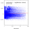 |
Fig. 1. Airmass effect correction for the Ca II H & K index. |
3. Data analysis
3.1. Periodogram analysis
Figure 2 (left) shows the temporal variations of the analysed activity indexes. The median index per day is shown. From now on, we refer to the median index per day in all the analysis performed. A search for periodicities was performed by using the generalised Lomb-Scargle periodograms (GLS, Zechmeister & Kürster 2009). The periodograms are dominated by long-term signals. In order to clearly identify signals at the solar rotation period, we subtracted the main long-period trends for each index by fitting a sinusoidal function (a procedure usually referred to as prewhitening). The subtracted periods are close to 27000 days for Ca II, and Hϵ, near 3800 days for Hα, and of the order of 1200 days for Hβ, Hγ and Hδ. Additional long-term signals with periods between 200 and 600 days were removed from most of the indexes. The subtracted periods as well as the number of prewhitenings performed are given in Table 2 while Fig. 2 (right) shows the corresponding GLS periodograms. Periods were subtracted in a sequential way, until a period inside the time interval of the Sun’s rotation (between 25 and 34 days) dominates the periodogram. For example, for the S index, the period labelled as P1 in Table 2 was subtracted, while for Hβ the periods labelled as P1 and P2 were prewhitened. We note that the time series are those of the original datasets, that is, before any prewhitening procedure is applied, while we show the periodograms after the described prewhitening procedure. Several conclusions can be drawn from this figure. First, long-periods still remain, in particular for the Hβ index. Second, the solar rotation is found in all activity indicators with the exception of Hδ where it is not clearly detected and which shows a lot of periods close to 22 days. The most significant periods that we identify with the solar rotation for each index are given in Table 2. Their uncertainties are those provided by the GLS analysis. We note that these are synodic periods and therefore not corrected from effects due to the Earth’s revolution around the Sun. Our results show that the rotation period depends on the indicator used. It varies from 26.29 days (Hγ index) to 31.23 days (He I).
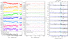 |
Fig. 2. Activity indexes time series and periodograms. Left: activity indexes (defined in the text) as a function of time. Daily median values are shown. Centre: zoom on the time series covering a period of two rotations. Right: corresponding generalised Lomb-Scargle periodograms (after the subtraction of the main long-term periods, see text for details). The light blue lines indicate the solar synodic period of 27.2753 days (Allen 1977) while values corresponding to a FAP of 10%, 1%, and 0.1% are shown with dashed lines. |
Periods found in the GLS periodogram analysis, assumed rotation periods, and relative spread in rotation period α, potentially indicative of differential rotation, measured from the sliding periodograms for the different activity indicators.
Figure 2 also reveals an increase in the Hβ, Hγ, and to a lesser extent Hδ values at BJD approximately equal to 2457800 days. Then, around BJD 2458100 days the indexes show a small decline. These values do not correspond to the period of reduced S/N. We checked whether large plages were present in the solar surface at these epochs by carefully analysing the USET images2 at the Solar Influence Data Analysis Center of the Royal Observatory of Belgium as well as the NASA/SDO AIA 1600 images3. We find that while at BJD around 2457800 days the solar surface does not differ in a significant way from other epochs, at BJD around 2458000 days (where the Hβ index shows a peak) several active regions (with associated NOAA numbers from 12673 to 12677) formed by plages and dark spots are visible across the solar surface.
Furthermore, for the He I, Na I, and perhaps Hα lines several periods of low values can be seen. As they are separated by approximately 350 days we suspect that this effect could be related to the presence of weak telluric lines contaminating the cores or continua of these indexes and thus inducing annual variations.
We finally study the impact of the prewhitening in the determination of the rotation period. This is illustrated in Fig. 3 where we show the periodograms corresponding to the S index (left panel) and Hα index (right panel) after each prewhitening. The plot shows a zoom around the region of the solar rotation. It is clear from the figure that the prewhitening procedure does not change the found periods, only their relative strength. The GLS power of the periods increase after each prewhitening. The periodogram corresponding to the S index show a more complex pattern than in the Hα case. For the S index three main periods at 26.30, 27.31, and 28.62 days are clearly dominant in all cases. The latest period is broad and seems to be mixed with a close period at 29.44 days. In addition, two secondary peaks appear at 25.33 and 32.08 days, respectively. Regarding Hα, another three period structure can be seen that dominates the periodogram with power at approximately 26.57, 29.42, and 32.58 days. We note that the period at 32 days which is dominant in Hα is also seen in the S index, although it is not among the dominant signals for this indicator. The other main difference between the S index and Hα periodograms is that the periods at approximately 27.3 days and 26.3 days which are dominant in the S index are much less significant in the Hα data.
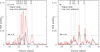 |
Fig. 3. GLS periodograms of the S (left) and Hα indexes (right) after each prewhitening zoomed around the periods of interest. Vertical dashed-to-dot lines show the periods discussed in the text. |
3.2. Temporal evolution of active regions
In order to study the temporal evolution of active regions we made use of the pooled variance technique (Donahue et al. 1997a,b; Lanza et al. 2004; Scandariato et al. 2017). In brief, for a given time interval, t, the data are binned into segments of length t, and the average variance of the set of these segments is computed. It is expected that as the time scale increases, the effects from processes at longer time scales become more noticeable and therefore the pooled variance increases.
For example, the light curve of a star with a fixed, non evolving, spot pattern and rigid rotation will be perfectly periodic. The variance of this light curve will increase with t, until Prot is reached. For timescales longer than the rotation period, the mean variance will stay approximately constant. If we now introduce the evolution of active regions, and the timescale of evolution is significantly longer than Prot, the variance of the light curve will increase for timescales longer than Prot until the mean timescale of evolution of the active regions is reached. We will have a change in slope because the increase of the variance with t is generally different from that produced by rotation, given that the shape of the rotational modulation is different from the light changes associated with active region evolution.
The corresponding pooled variance diagrams for the activity indexes analysed in this work are shown in Fig. 4. The pooled variance was computed from t = 5 days up to one third of the total time of the observations, with a time step of 10 days. The analysis of the data shows two slope changes, one around 30 days which corresponds to the solar rotation period and a second one around 300 days from which we infer a typical lifetime for active regions of approximately 10 rotation periods. We note that the second slope change around 300 days is not so strong in the He I and Na I activity indicators. The time scale of approximately 300 days is quite similar to the mean life time of complexes of activity dominated by faculae and plage (e.g. Castenmiller et al. 1986) while sun spots are known to live for hours to months (e.g. Solanki 2003). We finally note the peculiar behaviour of the Hα index, which shows almost no variation after 300 days in contrast to the other indexes.
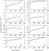 |
Fig. 4. Pooled variance diagrams for the different activity indicators analysed in this work (see text). The red line is a smoothed function for ease reading of the plots. |
We study solar rotation via time-varying periodogram power of the activity indexes. Power spectra are computed for each activity index time series in overlapping segments of 600 days, with a two day time shift between consecutive segments. Before computation, the long-term periods identified in the GLS analysis described above were prewhitened in a sequential way. Additionally, we perform a linear detrending of the data in each 600 days temporal window independently. The corresponding sliding periodograms are shown in Fig. A.1.
We note that a large window is needed if we want to average the effect of the different surface inhomogeneities (e.g. Bertello et al. 2012). Figure A.2 shows the corresponding sliding periodogram for the S index computed using a temporal window of 300, 600, and 900 days, respectively. Although similar in form, that is, the Scargle power is found at roughly the same periods, it is clear from the figure than when using a small temporal window the revealed signals tend to be broader. In addition, discontinuities appear for periods larger than approximately 40 days. If a window of 900 days (i.e. almost the full temporal coverage of our data) is considered (bottom panel) the periods appear significantly narrower, but many white vertical strips (meaning that no temporal window is centred at the corresponding date) appear in the plot. We note that gaps in the data should not been quite different from one window size to another. After all, all windows are quite large. However, with increasing the temporal window we are covering a shorter global time scale (i.e. we are making a kind of zoom, see the range of dates in the X axis for the different plots of Fig. A.2) so the gaps in the data are more easily seen in the plots. We choose 600 days as a compromise between having a large temporal window (so periods are narrow enough) and having a large temporal coverage. We also investigated whether the prewhitening procedure performed to the data does have an impact on the sliding periodograms. This is illustrated in Fig. A.3 where sliding periodograms for the S index are shown for the original time series (up panel), and after prewhitening the long-term signal (middle panel), see Table 2 for the exact values of the subtracted periods. We can see that the periodograms are nearly identical, with only very small differences. We conclude that the prewhitening procedure has a small impact on the periodograms.
We use the periodograms to search for a signature of differential rotation. Table 2 shows the spread in rotation periods, α, defined as (PMax − PMin)/PMax being PMax and PMin the maximum and minimum rotation periods. It was measured by visual inspection of the drift in the mean frequency of the forest of peaks around the rotation frequency. Uncertainties on α are computed by assuming an error on PMax and PMin of 0.07 days (median values of the errors in the periods listed in Table 2) and applying uncertainties propagation. These uncertainties are clearly underestimated. This is because our real uncertainty depends on the choice of PMax and PMin which in turn rely on the noise level of each index. This effect might lead to a lower α value as peaks on the outside are in general weaker and most likely to be missed. Furthermore, a period which is present in one index might not be present in another index with a higher level of noise. The value of α depends significantly on the index. It is higher for the S index and Hϵ. We note that for Hδ and He I we were not able to determine α. That (in addition to the previous results) suggests that either the Hδ line is less sensitive to stellar activity than other indicators or that the definition of this index should be revised. Finally, for Hγ the value of α was derived from the first harmonic of the rotation period.
It is important to note that we cannot unambiguously attribute the splitting of the rotation period peaks to differential rotation. It is well known that spot or active region evolution can induce similar beat patterns, broadening or splitting peaks in the periodograms (e.g. Lanza et al. 1994; Aigrain et al. 2015). As discussed, we measured typical activity complex lifetimes of 10 rotation periods. However, the presence of small-scale features evolving over shorter timescales cannot be excluded. The presence of several close periods might, indeed, be a combination of differential rotation and spot evolution.
In addition to the periods inside the 20−36 days time interval of the Sun’s rotation, other periodicities are found in the sliding periodograms, see Fig. A.1. In particular, one period at approximately 14.5 days is visible in most of the indicators, specially in Hγ. When considering the S index, a secondary peak close to 13.5 days is also visible. We believe that these features might correspond to a 12−14 days periodicity previously identified in the literature. This period has been shown to be an effect of an active longitude, that is the result from two different active regions separated by 180° in longitude (Donnelly 1988; Donnelly & Puga 1990; Bouwer 1992). The harmonic of the rotation period is also present and both effects contribute to this signal. It is also partly caused by the light curve of a single spot being similar to a truncated sinusoid (it is flat when the spot is on the invisible hemisphere).
A period at approximately 18 days is seen in Hα. To the best of our understanding, no reference to such a period has been found in the literature. Periodicities around 43.5 and 47.5 days are visible in the S index analysis, in agreement with previous works (e.g. Ziȩba et al. 2001). For Hγ a periodicity close to 51 days is found. The origin of this periodicity at 51 days is still unclear, although it seems that it appears most strongly in measurements related to emerging magnetic flux (Bouwer 1992).
Finally, several signals at larger periods are found. For the S index, there is a signal ranging from 70 to 76 days, as well as another one from 86 to 92 days. Additional signals around 125 and 135 days also appear in the periodogram of the S index. A clear signal at 100 days is seen in Hγ, while Hϵ show a signal at approximately 80 days and another one ranging from approximately 98 to 113 days. Signals at these periods have already been reported in other solar studies (e.g. Ziȩba et al. 2001).
Another clear signal at approximately 170 days appears in the periodogram of the S index. This periodicity is a bit longer to the so-called Rieger cycles discovered in the periodicity of high-energy solar flares Rieger et al. (1984) and it has been also found in indicators for solar activity such as sunspot areas (e.g. Oliver et al. 1998). It has a periodicity around 155−160 days, and it usually appears only near the maxima of solar cycles. Zaqarashvili et al. (2010) suggested that this periodicity might be connected to the dynamics of magnetic Rosbby waves in the tachocline.
We finally comment on the large period of 31.23 days derived from the analysis of the He I time series. This line is known to be formed at somewhat higher temperatures than other optical diagnostics of activity (Saar et al. 1997) and it is often used to study prominences and flares (Zirin 1988). We note that such a period would correspond to active regions located at significant high latitudes, approximately 60° (but see next section). From Fig. 2 it can be seen that its significance level is lower (false alarm probability, FAP approximately 1%) than the periods corresponding to other indexes that show FAP values highly below 0.1%. This is also evident in the corresponding sliding periodogram, Fig. A.1 (bottom left panel) where the period is not seen, as only periods with FAPs lower than 0.01 are shown. Instead, two periods are clearly visible, although only at the end of the observing window. These are the period at 12−14 days discussed above, and another period at approximately 40 days.
3.3. Comparison with previous work
It is not straightforward to determine the rotation period from a periodogram analysis. For the Sun, we usually take advantage of the fact that we already know the value of the rotation period we are searching for (see Hall & Lockwood 1998). An early attempt to measure the solar surface differential rotation of the Sun-as-a-star was made by Donahue & Keil (1995) based on the periodogram analysis of Ca II K disc-integrated data. The authors reproduce the expected behaviour of the rotation period with time (with periods ranging from 22.8 to 28.0 days) with an abrupt jump in period in the transition between cycles 21 and 22. They also studied the pooled variance, finding that the evolution of active regions contribute to the total variance of the disc-integrated Ca II K line at time scales from 20 to 400 days, which is a time scale compatible, although slightly longer time scale, than our results, see Fig. 4.
Hempelmann & Donahue (1997) performed a wavelet analysis of disc-integrated solar Ca II K line core emission measurements. The authors found the solar synodic rotation with a maximum power at a period of 28.3 days corresponding to the solar rotation at latitude 30°. They also found a second (less dominant) period at 26.8 days as well as a third peak at 30.2 days related to the existence of active regions at 5° and 50°, respectively. Our data, see Fig. 2, shows a period of 27.31 days as the dominant one, while secondary peaks at 28.62 and approximately 26.30 days also appear. Using the known relationship between solar rotation rate and latitude it is possible to estimate the latitude of active regions at which our peaks would correspond. There is a large amount of determinations of the solar rotation rate which depend on the methods and the type of data used, that is, the type of feature used as a tracer, for a review see Beck (2000). It is known that chromospheric indicators provide higher rotation rates than those based on photospheric disc observations. This can be easily shown by comparing the equatorial rotation rates provided in Table2 (based on measurements of solar features) and Table 1 (spectroscopic measurements) provided by Beck (2000). It is also clear from Table 2 that our assumed rotation periods are more similar to the values derived from Table 1 of Beck (2000). Snodgrass & Ulrich (1990) derived three relationships, one related to magnetic features, a second one that refers to the rotation of supergranules (which are found to rotate faster than magnetic structures), and a third spectroscopic (i.e. based on doppler measurements of spectral features) relation. Using the coefficients provided by the latest relationship, our peaks would correspond to active regions located between the equator and 30°.
We have checked whether this could be the case by analysing the available data on active regions and solar spots at the Heliophysics Feature Catalogue4. Given the dates of our observations, the beginning of our time series should correspond to a fast rotation rate, while the end to a low rotation rate. At the beginning of our observations, active regions were located at latitudes between −30° and 20° and sunspots were distributed into two regions between −10° and −20° and between 10° and 20°. At the end of our observing window, active regions are mostly located between −10° and 20°, while spots are seen into three groups at −10°, 5°, and 15°, respectively. We conclude that the presence of active regions located between the equator and 30° are indeed a plausible explanation for the observed periods. We also see that there seems to be no significant variation in the maximum latitude of active regions during our observation window.
In their wavelet analysis, Hempelmann & Donahue (1997) found three bands of periods at around 26, 28, and 30 days. This is consistent with our sliding periodogram shown in Fig. A.1 where we see three main periods at around 26, 28, and 30 days. A fourth period beginning at approximately 32 days is also visible.
More recently Bertello et al. (2012) measured disc-integrated Ca II K line and observed periods in the range between 27.7 and 28 days. They find most of the power spectral density concentrated into a narrow band, whose central value varies in the range 26.3−28.6 days, consistent with the migration of active regions from latitudes between 30 and 35° to the equator. This result is consistent with the findings from our work. It is worth noticing that while these authors found a single narrow band in their spectral analysis, the results from our power spectra are split into several main bands. Bertello et al. (2012) noted that while parameters defined in terms of wavelength separation show a spectrum with a single predominant peak, intensity-related parameters (like our measured indexes) show a power spectrum with a more complex pattern. Further differences can arise from the spectral estimator used by these authors (the maximum entropy method) that seems to produce less complex spectral patterns than the generalised Lomb-Scargle periodogram used here.
Other attempts to measure the solar differential rotation have been performed using a combination of UV and optical lines using UARS SOLSTICE data (Hasler et al. 2002; Hempelmann 2002) but no clear signatures of differential rotation were detected. We note that this result refers to integrated light. Using Sun-as-a-star radial velocities measured during an eclipse, Takeda et al. (2015) tried to determine the coefficients of the solar rotation law5 finding a relationship between the coefficients A, and B. However, an individual estimate of the parameters A and B were not possible.
Livingston (1969) noted an increase of the order of 8% of the angular velocity measured in the chromospheric Hα line with respect to other photospheric lines. Regarding the activity indexes measured in this work, Na I D1 D2 is known to form in the upper photosphere and lower chromosphere, Hα, Hβ, and Ca II H & K in the middle cromosphere, while He I D3 is formed in the upper chromosphere (e.g. Montes et al. 2000). No clear relationship between formation height and rotation rate is seen in our data. This conclusion is based on three facts: (i) the rotation period derived from the Na I D1 D2 is similar to the one from Hβ; (ii) Hα show a higher period (between 2.5 and 7%) than Ca II and Hβ; and (iii) as discussed above the rotation period found for the He I index is less significant. Nevertheless, we acknowledge that further studies should be performed, in particular the analysis of photospheric and coronal lines as well as a better knowledge of the lines’ formation height would help to clarify this issue. We also tried to plot the assumed rotation period as a function of the line’s excitation potential but no clear trend was evident. We finally checked for a tendency with the quantum number within the Balmer series, where Hα show a higher period than Hβ and both lines provide higher rotation levels than Hϵ. Unfortunately, we were not able to detect the rotation period in Hδ and the rotation period of Hγ does not follow this tendency.
3.4. Correlation between activity indexes
We also investigated the correlations between the different activity indexes described in Table 1. Using the code MCSpearman6 (Curran 2014) we calculated correlations using a bootstrap Monte Carlo by adding a Gaussian random variate with standard deviation equal to the measurement uncertainty to each data point. For each pair of activity indexes, the corresponding Spearman coefficient correlation, ρ, and its z-score7 were determined from 104 synthetic datasets. Figure 5 shows the correlations between the different activity indexes, and the results from the statistical tests are provided in Table 3. We note that the analysis presented in this section was made on the original time series (i.e. without any prewhitening applied).
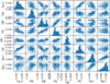 |
Fig. 5. Correlation plot between the different activity indexes. The diagonal panels show the histogram of each index. |
It can be seen that Hα, Hβ, Hγ, and He I show a significant anti-correlation with the S index although the correlation coefficients are rather modest: 0.3−0.5. The Hϵ line, however, shows a positive correlation. Hδ, and Na I show no statistically significant correlation with the S index.
Table 3 also reveals that the strongest correlation is typically with the closest index in wavelength (i.e. Ca II with Hϵ, Hα with He I, Na I with HeI, and Hβ with Hγ). While this could be an instrumental effect (scattered light as a function of wavelength), if real, it could indicate a dependence on the formation height of the different indexes.
Correlations between the activity indexes as defined in the text.
As mentioned, one result from Fig. 5 and the analysis presented in Table 3 is that S emission and Hα seem to anti-correlate. This might be an unexpected behaviour as both quantities are well known to correlate with the solar cycle (e.g. Livingston et al. 2007; Meunier & Delfosse 2009) and a good correlation between the S index and Hα has been found for other stars (Flores et al. 2016). However, it should be noted that these first works are based on nearly thirty and twenty years of observations, while the short-term correlation between S and Hα and its relationship with the level of activity is still not well understood (e.g. Giampapa et al. 1989; Strassmeier et al. 1990; Robinson et al. 1990; Montes et al. 1995). It is also worth noticing that a wide variety of correlations between −1 and +1 have been found in other stars with spectral types between F6 and M5 (Cincunegui et al. 2007; Gomes da Silva et al. 2011, 2014). It has also been shown that stars exhibiting a positive correlation show a tendency to be more active and that negative correlations are more present among higher metallicity stars (Gomes da Silva et al. 2014). In particular, we note that these authors found that stars more active than logR′HK = −4.7 showed positive correlations, while the median solar value is −4.907 (Mamajek & Hillenbrand 2008). Although the Sun is not a metal-rich star, we note that these authors found negative correlations even in stars with [Fe/H] values as low as −0.15 dex.
In order to test whether the negative correlation coefficient between S and Hα is related to the time scale of the observations we study how the correlation depends on the timescale of the observations. This is shown in Fig. 6. The correlation between S and Hα is computed for different time intervals and different starting times in the series (i.e. different cycle phases). For each time interval, individual circles correspond to a different starting time in the series. We overplot with red stars the lower boundary of the data presented in Meunier & Delfosse (2009, Fig. 3) while with green stars we show the upper boundary. The figure shows that shorter time lags lead to more negative correlation coefficients. In particular, negative correlation coefficients as the ones obtained in this work are consistent with the findings of Meunier & Delfosse (2009). However, unlike these authors we are not able to obtain correlations close to one in any of the inspected time lags.
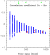 |
Fig. 6. Correlations between the S and Hα activity indexes as a function of the time span. Red and green stars denotes the lower and upper boundary of the data shown in Meunier & Delfosse (2009, Fig. 3). |
We conclude that correlation coefficients as low as approximately −0.30 can be obtained for short timescales in agreement with previous results. However, the question of why we do not get any value close to one remains open. At this point two explanations are possible: either the two lines show a different response to increasing activity or the correlation between S and Hα depends on the level of activity. We should note that the data by Meunier & Delfosse (2009) covers almost 30 years of observations, so they can really test different parts of the solar cycle in each temporal window. However, our observations do cover approximately 2.9 yr so even if we choose different starting times we do not trace different parts of the cycle, only the end of the decreasing phase and around the minimum. This is specially evident when large windows are considered, for example, if a window including 900 days is explored, starting dates can not be separated by more than 32 days, so we are essentially in the same phase of the cycle.
Regarding the behaviour of Ca II and Hα with activity, it is well known that the Hα line is radiation-dominated and it first shows a deeper absorption profile as activity increases until the electron density is high enough and the line becomes collisionally excited, then increasing the emission at its core. On the other hand, chromospheric Ca II H & K emission lines are collisionally dominated, thus the radiated flux steadily increases with electron pressure (Cram & Mullan 1979; Cram & Giampapa 1987; Rutten et al. 1989; Houdebine et al. 1995; Houdebine & Stempels 1997; Scandariato et al. 2017). On the other hand, the dependency of the correlation between S and Hα with the level of activity is discussed at length in Sect. 4.
Some degree of correlation between Ca II and Hα is however visible in our data. This can be seen in Fig. 2. At the beginning of the time series, the S index shows a variation due to the crossing of active regions (we have checked using solar images that several active regions were effectively crossing the solar disc during these days). This is also visible in Hα. There seems to be a correspondence between peaks in both indexes, although the higher noise level in the Hα index makes the comparison difficult. Another hint of correspondence between peaks in both indexes can be seen in the middle panel of Fig. 2 which shows a zoom around BJD = 2458000 days. We should note that we do not have a clear reason of why the Hα time series is noisier. We expeculate that it could be related to contamination by some non-corrected nearby telluric line. Whether the higher noise level in the Hα data might contribute to hide a clearer S index and Hα correlation is unclear. As mentioned, there are other factors that should be considered.
The results from the He I and Na I indexes also deserve further comments. In particular, we should note that clear cyclic variations in the Na I index have been found for the Sun (Hall & Lockwood 1998; Livingston et al. 2007) and a clear correlation between Na I and the S index in low activity M dwarfs has been reported (Gomes da Silva et al. 2011). However, from our results no statistical significant correlation is found between these two indexes. Regarding He I measurements, we find a statistical significant anti-correlation with the S index, while He I observations of the 1083 nm line have been shown to show variations correlated with the solar cycle (Livingston et al. 2007). We should note that the He I line at 1083 nm has been shown to be negatively correlated with activity, that is, it becomes deeper when the Sun is more active (Andretta & Giampapa 1995), in line with the findings of our work. Furthermore, Gomes da Silva et al. (2011) found little variation of He I index (measured in the same line than our work) as well as a low correlation with activity, although their results refers to M dwarfs.
We believe that as might happens with the Hα the lack of a clear (positive) correlation of these indexes with the S index is due to the relatively small temporal window covered in this work as well as a possible dependence of the correlations on the level of activity, we note that our observations cover the decreasing phase and the minimum of the solar cycle. Furthermore, these indexes also show higher levels of noise.
We finally caution that the presence of etalon ripples on the HARPS-N solar data has been reported (see Thompson et al., in prep.). In order to understand whether they can effect the correlations between activity indexes we took several random spectra and computed the GLS periodogram of 50 and 100 Å width regions centred around the activity indexes, finding no evidence of ripples in these regions. At the time of writing, we are not aware of any other possible anomaly in the data that might affect our measurements. A future analysis of the solar images covering the same time span analysed in this work would be helpful to clarify the trends between the different activity indicators found in this work as well as the different significance levels of the periods found in these indexes.
3.5. Correlation activity indexes – CCF parameters
Possible correlations between the RVs and several CCF asymmetry diagnostics were also investigated. We considered the CCF width (FWHM), the bisector span (Queloz et al. 2001, BIS), and its contrast. The heliocentric radial velocity (as described in Sect. 2) was also considered. In addition, FWHM values were also corrected to the sidereal frame, see Cameron et al. (2019). Spearman correlation coefficients, ρ and z-scores for these correlations are given in Table 4, and Fig. 7 shows the correlations for the Ca IIS index. The analysis presented in this section corresponds to the original time series (i.e. without any prewhitening applied).
Correlations between the different activity indexes and the CCF indexes.
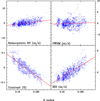 |
Fig. 7. CCF parameters vs. the Ca II H & K index. Best linear fits are shown in red lines. |
We search for significant correlations using a z-score larger than 3.0 in absolute value, the usual threshold for statistical significance. These are shown in bold face in Table 4. The Ca II index shows a significant correlation with the bisector and the heliocentric RV values while it shows an anti-correlation with the contrast. A similar behaviour is seen for the Hϵ line. Also Hβ shows the same correlations but in all cases with the opposite sign. Additional significant correlations are found between the Hα index and the CCF contrast and between the Hγ and Na I indexes and the contrast and bisector (with opposite signs). Furthermore, the He I index also correlates with the CCF contrast. No correlations are found between the Hδ index and the CCF parameters.
It is important to note the positive correlation between the heliocentric radial velocity and the activity index S. Our derived Spearman’s correlation coefficient of 0.40 ± 0.03 (with a 5.1σ confidence level) is in agreement with the value of 0.357 found by Lanza et al. (2016). The rms of the RV variations is 4.9 ms−1, also in agreement with these authors. Time delays between the FWHM and BIS values with the RV variations have been predicted by models (Dumusque et al. 2014) and found in the HARPS-N solar data by Cameron et al. (2019). We searched for similar time delays between the S index and RV variations but no evidence was found. The correlation between the emission in the Ca II line and the radial velocity supports the idea of the quenching of local convective motions in active regions being the main effect on the Sun-as-a-star radial velocities, as predicted by Meunier et al. (2010a) and Meunier & Lagrange (2013). This has been observationally confirmed by Haywood et al. (2016) and Milbourne et al. (2019). On the other hand, the effect of inhomogeneities in the solar surface (such as dark spots or bright faculae) can be either positive or negative depending on the filling factors and the location of active regions (receding or approaching half of the solar disc), leading to a weaker S index – RV correlation (Lagrange et al. 2010; Meunier et al. 2010a,b; Dumusque et al. 2014).
Along these lines, Haywood et al. (2016) searched for correlations between the RV variations of the Sun-as-a-star and the RV component due to the suppression of the convective blueshift with the log(R′HK) values. When considering the overall RV, they find a correlation coefficient of 0.18, i.e, significantly lower than our value, while the coefficient increases to 0.35 (more similar to our value) when only the RV due to the suppression of convective blueshift is taken into account. It is important to note that this comparison may be biased by the fact that the radial velocities from this previous work were taken at a different time in the activity cycle (in particular the Sun was more active than in our observing season), so the fact that we obtain similar correlation coefficients to the Haywood et al. (2016) values might be coincidental. We note that the data by Haywood et al. (2016) were collected from September 29 to December 7, 2011 and were spread over 38 nights for a total of 98 datapoints. In addition, the first part of the RV data suffered from an additional scatter owing to the finite diameter of the asteroid 4/Vesta being comparable with the fibre diameter on the focal plane.
In a recent work Lanza et al. (2018), studied the correlations of different CCF indicators, in particular the FWHM and the BIS, with the radial velocity variations for a sample of 15 solar-type stars. The authors found significant correlation in 13 (FWHM) and 27 (BIS) percent of the stars. A search for similar correlations were performed in our data. The results are shown in Fig. 8 where the FWHM and BIS values are plotted against the heliocentric radial velocity. Our analysis reveals a significant positive correlation between the FWHM and the BIS with the heliocentric radial velocity. For the FWHM the Spearman’s rank coefficient is 0.267 ± 0.033 with a z-score value of 3.310 ± 0.429. When considering the BIS values, we obtain a Spearman’s rank coefficient of 0.325 ± 0.032 and a z-score value of 4.075 ± 0.435.
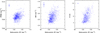 |
Fig. 8. Sidereal FWHM (left), bisector span (centre), and disc-integrated magnetic flux (right) as a function of the heliocentric radial velocity. |
Finally, we studied the relationship between the mean magnetic flux derived from SOLIS/VSM full-disc line-of-sight magnetograms which correspond to the core of the photospheric 630.15 nm Fe line (Jones et al. 2002)8 and the heliocentric radial velocity. The corresponding plot is shown in the right panel of Fig. 8. A significant correlation is found with a Spearman’s rank coefficient of 0.463 ± 0.04 and a significance z-score of 5.026 ± 0.452. We note that our derived Spearman’s coefficient is significantly larger than the 0.131 found by Lanza et al. (2016), and is in agreement with the 0.58 value found by Haywood et al. (2016). It is lower than the 0.87 value found when only the radial velocity contributions from convective blueshift (the factor that dominates the radial velocity of the Sun-as-a-star) is considered (Haywood et al. 2016).
4. Discussion
The temporal variation of the correlations coefficients described in Sects. 3.4 and 3.5 was also studied. As in Sect. 3.2, correlations tests were performed considering a large window of 600 days period of observations every two days. We focus on two correlations: those between Hα and the Ca II H & K indexes and between the heliocentric RV and the Ca II H & K index. The top of Fig. 9 shows variations in the correlation of these quantities changes with time.
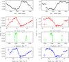 |
Fig. 9. Slope of the relationship between Ca, and Hα indexes (left), and slope of the relationship between Ca, and the heliocentric RV (right) as a function of time, the sunspot index, the solar irradiance, and the solar radio flux. |
4.1. Understanding the Ca – Hα correlation
In order to understand the correlations between the emission in the Ca II H & K and the Hα lines, in each temporal window the slope of the S versus Hα index relationship was computed. The slopes are then plotted versus the mean time of the temporal window as well as versus the mean values of different observables related to the evolution of magnetic structures in the solar atmosphere, Fig. 9 (left). These observables are (i) the daily total sunspot number by the Royal Observatory of Belgium9; (ii) the total solar irradiance data from the University of Colorado10; and (iii) the solar f10.7 radio flux from the University of Colorado11. While other possible diagnostics are available, they do not cover the dates of our HARPS-N observations.
In this analysis we use the original time series of the indexes. The figure reveals a tendency of less negative slopes as we move towards larger sun spot numbers, irradiance, or radio flux values. We finally tested whether the derived slope correlates with these quantities. For this purpose we use the procedure described in Sect. 3.4. The results are given in Table 5. It shows the correlation coefficient and z-score between the slopes (of the S index vs. Hα index relationship) and the sun spot, irradiance, and radio flux values. The results from this statistical test do not exclude that correlations are present but suggest that they are relatively weak. A dependence of the correlation between the S index and Hα with the level of activity has also been found in FGK stars (Gomes da Silva et al. 2014) as well as in a sample of early-M dwarfs by Gomes da Silva et al. (2011). It is interesting to note that Gomes da Silva et al. (2014) also found this correlation to be dependent on the stellar metallicity suggesting that negative correlations were present among higher metallicity stars, but as we are studying one single star we are not able to test this result.
Correlations between the slope of the S index and Hα relationship and different observables of the evolution of magnetic structures in the solar atmosphere.
It is well known that at short time scales the emission in the Ca II H & K and Hα do not always correlate. Meunier & Delfosse (2009) suggest that the presence of plages might lead to a correlation coefficient lower than one as the surface covered by the Hα plages is slightly smaller than the surface covered in Ca (the calcium lines are formed higher in the chromosphere), and that also the chromospheric network is more prominent in calcium. The different contrast of dark filaments in Ca and Hα might also decrease the correlation coefficient between Ca and Hα or even lead to an anti-correlation, if strong filaments correlated with plages are present (Meunier & Delfosse 2009). Indeed, it could be that filaments are actually more prominent in all Balmer’s lines, which might partly explain their anti-correlation with the Ca index (see Table 3).
Our results seem to be consistent with the scenario described above. At large sunspot numbers the emission in Ca and Hα show less negative slopes suggesting different relative contributions of the bright plages and dark filaments when compared to time intervals with a lower level of activity.
4.2. Understanding the Ca – RV correlation
We now search for correlations between the emission in the Ca II H & K and the heliocentric radial velocity. Figure 9 (right) shows the slope between the daily median S and the daily median heliocentric RV as a function of time and sunspot indexes.
A general tendency of a larger degree of correlation towards larger activity levels is present in the data, see Table 6, suggesting that a higher presence of surface inhomogeneities produces larger radial velocity variations. As mentioned, the correlation between the Ca II H & K and the heliocentric radial velocity is due to the suppression of convective blueshift by magnetic areas, leading to a net redshift. Therefore on cycle timescales, as total magnetic areas increase and decrease, the associated redshift will do likewise (e.g. Saar & Fischer 2000).
Correlations between the slope of the S index and heliocentric radial velocity relationship and different observables of the evolution of magnetic structures in the solar atmosphere.
It is worth noticing that the slope is not constant with time. That might be expected if larger filling fractions of magnetic regions effectively translate to larger radial velocity variations. Therefore, we conclude that there should be non-magnetic effects that swap the magnetic variations at epochs of low activity, thus reducing the apparent correlation.
5. Conclusions
In this work a detailed analysis of the main optical activity indicators including the Ca II H & K doublet, the Balmer lines, the Na I D1 D2 doublet, and the He I D3 measured in the Sun-as-a-star observations has been presented. Nearly three years of data were analysed.
The periodogram analysis of the data reveals the solar rotation period in almost all activity indicators with values ranging from 26.29 days to 31.23 days. The Hδ line is the only exception in which the rotation period was not found, suggesting that either this line is less sensitive to activity or that its definition should be revised. Furthermore, there is no clear reason why it does not correlate with other Balmer lines. The pooled variance analysis reveals two main slope changes. The first one is at around 30 days corresponding to the solar rotation period. The second slope change occurs at approximately 300 days, suggesting that the typical lifetime of complexes of activity dominated by plage and faculae is around 10 rotations periods, in agreement with previous results (e.g. Castenmiller et al. 1986). The study using sliding periodograms shows that the spectral power is usually split into several bands with periods ranging from 26 to 30 days. This effect might be due to differential rotation (migration of active regions between the solar equator and a latitude of approximately 30°), active region evolution, or a mixture of both phenomena. Again, no significant periods are found for the Hδ line.
We studied the correlations between the different activity indicators. Excluding Hδ and the Na II doublet, all the indicators show a modest but statistically significant correlation with the S index. In all cases, with the exception of Hϵ, the sign of the correlation is negative.
Significant positive correlations are found between the bisector and the heliocentric radial velocity with the S index and the Hϵ index, as well as an anti-correlation with the contrast. The Hβ line show similar correlations, but always with an opposite sign. Additional correlations with the bisector and the contrast and other activity indicators are also found. Further relationships between the FWHM, and the BIS with the radial velocity variations are found in agreement with previous results based on solar-type stars (Lanza et al. 2018). The disc-integrated magnetic field also is shown to correlate with the radial velocity variations as already found (Haywood et al. 2016; Lanza et al. 2016).
We finally focused on the temporal evolution of the S index and Hα correlation and the S index and radial velocity correlation. We show how these correlations depend on the presence of inhomogeneities on the solar surface (as measured by sun spot numbers, irradiance, and radio flux values). At larger levels of activity Ca and Hα (and Ca and radial velocity variations) show a higher degree of correlation, suggesting significant changes in the relative contributions of bright plages and dark filaments.
Combining the results from this work with additional studies of solar observations will help us to improve our understanding of stellar signals, allowing us to develop mitigation techniques that could be used to confirm small planets around low-mass stars. In particular, an in-depth analysis of solar images would help us to unravel the correlation between the S and Hα indexes, and to better understand the behaviour of these lines in the minimum phase of the activity cycle.
IRAF is distributed by the National Optical Astronomy Observatories, which are operated by the Association of Universities for Research in Astronomy, Inc., under cooperative agreement with the National Science Foundation.
ω = A + Bsin2ψ, where ψ is the latitude.
The z-score measures the degree of significance of the correlation. A z-score of z approximately corresponds to a Gaussian significance of the correlation of σ ∼ z.
Acknowledgments
J.M., A.F.L., G.M., A.S., L.M., E.M., G.P., and E.P. acknowledge the support by INAF/Frontiera through the “Progetti Premiali” funding scheme of the Italian Ministry of Education, University, and Research. D.F.P. is supported by NASA award number NNX16AD42G. X.D. is grateful to the Branco-Weiss Fellowship–Society in Science for financial support. A.C.C. acknowledges support from the Science and Technology Facilities Council (STFC) consolidated grant number ST/R000824/1. This work was performed in part under contract with the California Institute of Technology (Caltech)/Jet Propulsion Laboratory (JPL) funded by NASA through the Sagan Fellowship Program executed by the NASA Exoplanet Science Institute (R.D.H.) S.H.S. was supported by a NASA Heliophysics LWS grant NNX16AB79G. H.M.C. acknowledges support from the National Centre for Competence in Research (NCCR) “PlanetS” supported by the Swiss National Science Foundation (SNSF). L.M. acknowledges support from PLATO ASI-INAF agreement n.2015-019-R.1-2018. Based on observations made with the Italian Telescopio Nazionale Galileo (TNG), operated on the island of La Palma by the Fundación Galileo Galilei of the INAF (Istituto Nazionale di Astrofisica) at the Spanish Observatorio del Roque de los Muchachos of the Instituto de Astrofísica de Canarias. The solar telescope used in these observations was built and maintained with support from the Smithsonian Astrophysical Observatory, the Harvard Origins of Life Initiative, and the TNG. The HARPS-N project has been funded by the Prodex Programme of the Swiss Space Office (SSO), the Harvard University Origins of Life Initiative (HUOLI), the Scottish Universities Physics Alliance (SUPA), the University of Geneva, the Smithsonian Astrophysical Observatory (SAO), the Italian National Astrophysical Institute (INAF), the University of St Andrews, Queen’s University Belfast, and the University of Edinburgh. Based on SOLIS data obtained by the NSO Integrated Synoptic Program (NISP), managed by the National Solar Observatory, which is operated by the Association of Universities for Research in Astronomy (AURA), Inc. under a cooperative agreement with the National Science Foundation, data obtained by the WDC-SILSO, Royal Observatory of Belgium, Brussels, data obtained by the Solar Radiation and Climate Experiment (SORCE) satellite mission operated by the Laboratory for Atmospheric and Space Physics (LASP) at the University of Colorado (CU) in Boulder, Colorado, USA, and Penticton radio fluxes data from NOAA’s NGDC. We sincerely appreciate the careful reading of the manuscript and the constructive comments of the anonymous referee.
References
- Aigrain, S., Llama, J., Ceillier, T., et al. 2015, MNRAS, 450, 3211 [NASA ADS] [CrossRef] [Google Scholar]
- Allen, K. W. 1977, Astrophysical Quantities (London: Athlone Press) [Google Scholar]
- Andretta, V., & Giampapa, M. S. 1995, ApJ, 439, 405 [NASA ADS] [CrossRef] [Google Scholar]
- Baranne, A., Queloz, D., Mayor, M., et al. 1996, A&AS, 119, 373 [NASA ADS] [CrossRef] [EDP Sciences] [Google Scholar]
- Beck, J. G. 2000, Sol. Phys., 191, 47 [NASA ADS] [CrossRef] [Google Scholar]
- Bertello, L., Pevtsov, A. A., & Pietarila, A. 2012, ApJ, 761, 11 [NASA ADS] [CrossRef] [Google Scholar]
- Bouwer, S. D. 1992, Sol. Phys., 142, 365 [NASA ADS] [CrossRef] [Google Scholar]
- Cameron, A. C., Mortier, A., Phillips, D., et al. 2019, MNRAS, 1180 [Google Scholar]
- Castenmiller, M. J. M., Zwaan, C., & van der Zalm, E. B. J. 1986, Sol. Phys., 105, 237 [NASA ADS] [CrossRef] [Google Scholar]
- Cincunegui, C., Díaz, R. F., & Mauas, P. J. D. 2007, A&A, 469, 309 [NASA ADS] [CrossRef] [EDP Sciences] [Google Scholar]
- Cram, L. E., & Giampapa, M. S. 1987, ApJ, 323, 316 [NASA ADS] [CrossRef] [Google Scholar]
- Cram, L. E., & Mullan, D. J. 1979, ApJ, 234, 579 [NASA ADS] [CrossRef] [EDP Sciences] [Google Scholar]
- Curran, P. A. 2014, ArXiv e-prints [arXiv:1411.3816] [Google Scholar]
- Donahue, R. A., & Keil, S. L. 1995, Sol. Phys., 159, 53 [NASA ADS] [CrossRef] [Google Scholar]
- Donahue, R. A., Dobson, A. K., & Baliunas, S. L. 1997a, Sol. Phys., 171, 191 [NASA ADS] [CrossRef] [Google Scholar]
- Donahue, R. A., Dobson, A. K., & Baliunas, S. L. 1997b, Sol. Phys., 171, 211 [NASA ADS] [CrossRef] [Google Scholar]
- Donnelly, R. F. 1988, Ann. Geophys., 6, 417 [NASA ADS] [Google Scholar]
- Donnelly, R. F., & Puga, L. C. 1990, Sol. Phys., 130, 369 [NASA ADS] [CrossRef] [Google Scholar]
- Dumusque, X., Boisse, I., & Santos, N. C. 2014, ApJ, 796, 132 [NASA ADS] [CrossRef] [Google Scholar]
- Dumusque, X., Glenday, A., Phillips, D. F., et al. 2015, ApJ, 814, L21 [NASA ADS] [CrossRef] [Google Scholar]
- Fischer, D. A., Anglada-Escude, G., Arriagada, P., et al. 2016, PASP, 128, 066001 [NASA ADS] [CrossRef] [Google Scholar]
- Flores, M., González, J. F., Jaque Arancibia, M., Buccino, A., & Saffe, C. 2016, A&A, 589, A135 [NASA ADS] [CrossRef] [EDP Sciences] [Google Scholar]
- Giampapa, M. S., Cram, L. E., & Wild, W. J. 1989, ApJ, 345, 536 [NASA ADS] [CrossRef] [Google Scholar]
- Gomes da Silva, J., Santos, N. C., Bonfils, X., et al. 2011, A&A, 534, A30 [NASA ADS] [CrossRef] [EDP Sciences] [Google Scholar]
- Gomes da Silva, J., Santos, N. C., Boisse, I., Dumusque, X., & Lovis, C. 2014, A&A, 566, A66 [NASA ADS] [CrossRef] [EDP Sciences] [Google Scholar]
- Hall, J. C., & Lockwood, G. W. 1998, ApJ, 493, 494 [NASA ADS] [CrossRef] [Google Scholar]
- Hasler, K.-H., Rüdiger, G., & Staude, J. 2002, Astron. Nachr., 323, 123 [NASA ADS] [CrossRef] [Google Scholar]
- Hatzes, A. P. 2016, in Methods of Detecting Exoplanets: 1st Advanced School on Exoplanetary Science, eds. V. Bozza, L. Mancini, & A. Sozzetti, Astrophys. Space Sci. Lib., 428, 3 [Google Scholar]
- Haywood, R. D., Collier Cameron, A., Unruh, Y. C., et al. 2016, MNRAS, 457, 3637 [NASA ADS] [CrossRef] [Google Scholar]
- Hempelmann, A. 2002, A&A, 388, 540 [NASA ADS] [CrossRef] [EDP Sciences] [Google Scholar]
- Hempelmann, A., & Donahue, R. A. 1997, A&A, 322, 835 [NASA ADS] [Google Scholar]
- Henry, T. J., Soderblom, D. R., Donahue, R. A., & Baliunas, S. L. 1996, AJ, 111, 439 [NASA ADS] [CrossRef] [Google Scholar]
- Houdebine, E. R., & Stempels, H. C. 1997, A&A, 326, 1143 [NASA ADS] [Google Scholar]
- Houdebine, E. R., Doyle, J. G., & Koscielecki, M. 1995, A&A, 294, 773 [NASA ADS] [Google Scholar]
- Jones, H. P., Harvey, J. W., Henney, C. J., Hill, F., & Keller, C. U. 2002, in SOLMAG 2002. Proceedings of the Magnetic Coupling of the Solar Atmosphere Euroconference, ed. H. Sawaya-Lacoste, ESA SP, 505, 15 [NASA ADS] [Google Scholar]
- Lagrange, A.-M., Desort, M., & Meunier, N. 2010, A&A, 512, A38 [NASA ADS] [CrossRef] [EDP Sciences] [Google Scholar]
- Lanza, A. F., Rodono, M., & Zappala, R. A. 1994, A&A, 290, 861 [NASA ADS] [Google Scholar]
- Lanza, A. F., Rodonò, M., & Pagano, I. 2004, A&A, 425, 707 [NASA ADS] [CrossRef] [EDP Sciences] [Google Scholar]
- Lanza, A. F., Molaro, P., Monaco, L., & Haywood, R. D. 2016, A&A, 587, A103 [NASA ADS] [CrossRef] [EDP Sciences] [Google Scholar]
- Lanza, A. F., Malavolta, L., Benatti, S., et al. 2018, A&A, 616, A155 [NASA ADS] [CrossRef] [EDP Sciences] [Google Scholar]
- Livingston, W. C. 1969, Sol. Phys., 9, 448 [NASA ADS] [CrossRef] [Google Scholar]
- Livingston, W., Wallace, L., White, O. R., & Giampapa, M. S. 2007, ApJ, 657, 1137 [NASA ADS] [CrossRef] [Google Scholar]
- Lovis, C., & Pepe, F. 2007, A&A, 468, 1115 [NASA ADS] [CrossRef] [EDP Sciences] [Google Scholar]
- Lovis, C., Dumusque, X., Santos, N. C., et al. 2011, ArXiv e-prints [arXiv:1107.5325] [Google Scholar]
- Mamajek, E. E., & Hillenbrand, L. A. 2008, ApJ, 687, 1264 [NASA ADS] [CrossRef] [Google Scholar]
- Meunier, N., & Delfosse, X. 2009, A&A, 501, 1103 [NASA ADS] [CrossRef] [EDP Sciences] [Google Scholar]
- Meunier, N., & Lagrange, A.-M. 2013, A&A, 551, A101 [NASA ADS] [CrossRef] [EDP Sciences] [Google Scholar]
- Meunier, N., Lagrange, A.-M., & Desort, M. 2010a, A&A, 519, A66 [NASA ADS] [CrossRef] [EDP Sciences] [Google Scholar]
- Meunier, N., Desort, M., & Lagrange, A.-M. 2010b, A&A, 512, A39 [NASA ADS] [CrossRef] [EDP Sciences] [Google Scholar]
- Milbourne, T. W., Haywood, R. D., Phillips, D. F., et al. 2019, ApJ, 874, 107 [NASA ADS] [CrossRef] [Google Scholar]
- Montes, D., Fernandez-Figueroa, M. J., de Castro, E., & Cornide, M. 1995, A&AS, 109, 135 [NASA ADS] [Google Scholar]
- Montes, D., Fernández-Figueroa, M. J., De Castro, E., et al. 2000, A&AS, 146, 103 [NASA ADS] [CrossRef] [EDP Sciences] [Google Scholar]
- Oliver, R., Ballester, J. L., & Baudin, F. 1998, Nature, 394, 552 [NASA ADS] [CrossRef] [Google Scholar]
- Pepe, F., Mayor, M., Galland, F., et al. 2002, A&A, 388, 632 [NASA ADS] [CrossRef] [EDP Sciences] [Google Scholar]
- Phillips, D. F., Glenday, A. G., Dumusque, X., et al. 2016, Proc. SPIE, 9912, 99126Z [CrossRef] [Google Scholar]
- Queloz, D., Henry, G. W., Sivan, J. P., et al. 2001, A&A, 379, 279 [NASA ADS] [CrossRef] [EDP Sciences] [Google Scholar]
- Rieger, E., Share, G. H., Forrest, D. J., et al. 1984, Nature, 312, 623 [NASA ADS] [CrossRef] [Google Scholar]
- Robinson, R. D., Cram, L. E., & Giampapa, M. S. 1990, ApJS, 74, 891 [NASA ADS] [CrossRef] [Google Scholar]
- Rutten, R. G. M., Schrijver, C. J., Zwaan, C., Duncan, D. K., & Mewe, R. 1989, A&A, 219, 239 [NASA ADS] [Google Scholar]
- Saar, S. H., & Fischer, D. 2000, ApJ, 534, L105 [NASA ADS] [CrossRef] [PubMed] [Google Scholar]
- Saar, S. H., Huovelin, J., Osten, R. A., & Shcherbakov, A. G. 1997, A&A, 326, 741 [NASA ADS] [Google Scholar]
- Scandariato, G., Maldonado, J., Affer, L., et al. 2017, A&A, 598, A28 [NASA ADS] [CrossRef] [EDP Sciences] [Google Scholar]
- Snodgrass, H. B., & Ulrich, R. K. 1990, ApJ, 351, 309 [Google Scholar]
- Solanki, S. K. 2003, A&ARv, 11, 153 [Google Scholar]
- Strassmeier, K. G., Fekel, F. C., Bopp, B. W., Dempsey, R. C., & Henry, G. W. 1990, ApJS, 72, 191 [NASA ADS] [CrossRef] [Google Scholar]
- Takeda, Y., Ohshima, O., Kambe, E., et al. 2015, PASJ, 67, 10 [NASA ADS] [Google Scholar]
- West, A. A., & Hawley, S. L. 2008, PASP, 120, 1161 [NASA ADS] [CrossRef] [Google Scholar]
- Zaqarashvili, T. V., Carbonell, M., Oliver, R., & Ballester, J. L. 2010, ApJ, 724, L95 [NASA ADS] [CrossRef] [Google Scholar]
- Zechmeister, M., & Kürster, M. 2009, A&A, 496, 577 [NASA ADS] [CrossRef] [EDP Sciences] [Google Scholar]
- Ziȩba, S., Masłowski, J., Michalec, A., & Kułak, A. 2001, A&A, 377, 297 [NASA ADS] [CrossRef] [EDP Sciences] [Google Scholar]
- Zirin, H. 1988, Science, 242, 1586 [NASA ADS] [CrossRef] [Google Scholar]
Appendix A: Sliding periodograms
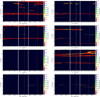 |
Fig. A.1. Sliding periodograms computed with a time window of 600 days. From left to right and from top to bottom: Ca II, Hα, Hβ, Hγ, Hδ, Hϵ, He I, and Na I. The X-axis shows the median time over which the GLS periodograms are calculated. Vertical white strips corresponds to gaps in the data. |
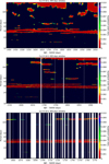 |
Fig. A.2. Sliding periodograms for Ca II computed with a time window of 300 (top), 600 (middle), and 900 days (bottom). The X-axis shows the median time over which the GLS periodograms are calculated. Vertical white strips corresponds to gaps in the data. |
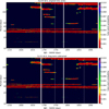 |
Fig. A.3. Sliding periodograms for Ca II computed for the original time series (top), and after prewhitening of the long-term period (bottom). The temporal window has been fixed to 600 days in all cases. The X-axis shows the median time over which the GLS periodograms are calculated. Vertical white strips corresponds to gaps in the data. |
All Tables
Periods found in the GLS periodogram analysis, assumed rotation periods, and relative spread in rotation period α, potentially indicative of differential rotation, measured from the sliding periodograms for the different activity indicators.
Correlations between the slope of the S index and Hα relationship and different observables of the evolution of magnetic structures in the solar atmosphere.
Correlations between the slope of the S index and heliocentric radial velocity relationship and different observables of the evolution of magnetic structures in the solar atmosphere.
All Figures
|
Fig. 1. Airmass effect correction for the Ca II H & K index. |
| In the text | |
|
Fig. 2. Activity indexes time series and periodograms. Left: activity indexes (defined in the text) as a function of time. Daily median values are shown. Centre: zoom on the time series covering a period of two rotations. Right: corresponding generalised Lomb-Scargle periodograms (after the subtraction of the main long-term periods, see text for details). The light blue lines indicate the solar synodic period of 27.2753 days (Allen 1977) while values corresponding to a FAP of 10%, 1%, and 0.1% are shown with dashed lines. |
| In the text | |
|
Fig. 3. GLS periodograms of the S (left) and Hα indexes (right) after each prewhitening zoomed around the periods of interest. Vertical dashed-to-dot lines show the periods discussed in the text. |
| In the text | |
|
Fig. 4. Pooled variance diagrams for the different activity indicators analysed in this work (see text). The red line is a smoothed function for ease reading of the plots. |
| In the text | |
|
Fig. 5. Correlation plot between the different activity indexes. The diagonal panels show the histogram of each index. |
| In the text | |
|
Fig. 6. Correlations between the S and Hα activity indexes as a function of the time span. Red and green stars denotes the lower and upper boundary of the data shown in Meunier & Delfosse (2009, Fig. 3). |
| In the text | |
|
Fig. 7. CCF parameters vs. the Ca II H & K index. Best linear fits are shown in red lines. |
| In the text | |
|
Fig. 8. Sidereal FWHM (left), bisector span (centre), and disc-integrated magnetic flux (right) as a function of the heliocentric radial velocity. |
| In the text | |
|
Fig. 9. Slope of the relationship between Ca, and Hα indexes (left), and slope of the relationship between Ca, and the heliocentric RV (right) as a function of time, the sunspot index, the solar irradiance, and the solar radio flux. |
| In the text | |
|
Fig. A.1. Sliding periodograms computed with a time window of 600 days. From left to right and from top to bottom: Ca II, Hα, Hβ, Hγ, Hδ, Hϵ, He I, and Na I. The X-axis shows the median time over which the GLS periodograms are calculated. Vertical white strips corresponds to gaps in the data. |
| In the text | |
|
Fig. A.2. Sliding periodograms for Ca II computed with a time window of 300 (top), 600 (middle), and 900 days (bottom). The X-axis shows the median time over which the GLS periodograms are calculated. Vertical white strips corresponds to gaps in the data. |
| In the text | |
|
Fig. A.3. Sliding periodograms for Ca II computed for the original time series (top), and after prewhitening of the long-term period (bottom). The temporal window has been fixed to 600 days in all cases. The X-axis shows the median time over which the GLS periodograms are calculated. Vertical white strips corresponds to gaps in the data. |
| In the text | |
Current usage metrics show cumulative count of Article Views (full-text article views including HTML views, PDF and ePub downloads, according to the available data) and Abstracts Views on Vision4Press platform.
Data correspond to usage on the plateform after 2015. The current usage metrics is available 48-96 hours after online publication and is updated daily on week days.
Initial download of the metrics may take a while.