© ESO 2019

1. Introduction

The cosmic microwave background (CMB) has proved invaluable for our understanding of early universe physics. Providing a direct image of the cosmos as it appeared only 380 000 years after the Big Bang, these fluctuations represent the initial conditions for all subsequent structure formation, eventually leading to the universe we observe today, consisting of galaxies, solar systems, and planets. Furthermore, through detailed statistical analysis of these temperature variations, cosmologists are today able to constrain many important cosmological parameters to percent-level precision (e.g., Planck Collaboration XIII 2016).

Steadily improving microwave detector technology has enabled this progress, resulting from a host of ground-based, sub-orbital, and satellite experiments. Amongst the latter are the most recent NASA’s Wilkinson Microwave Anisotropy Probe (WMAP) mission (Bennett et al. 2013) and ESA’s Planck mission (Planck Collaboration I 2016). The primary goal of all these experiments is to produce the cleanest possible image of the true cosmological CMB sky. However, when observing the sky at millimeter wavelengths, many other physical emission mechanisms contribute to the total sky brightness besides the CMB. The most important ones on large angular scales are synchrotron, free-free, thermal, and spinning dust, and CO emission, all of which arise from particles that are present within our own galaxy, the Milky Way (e.g., Planck Collaboration X 2015). On small angular scales, radio and far-infrared emission from distant galaxies are important, as is the Sunyaev–Zeldovich effect arising from hot gas in massive clusters. Collectively, all these signal are called “foregrounds” with respect to the CMB.

The process of extracting the cosmological signal from foreground-contaminated observations is often called CMB component separation, which informally refers to combining observations taken at different frequencies into a single estimate of the true cosmological sky. A wide range of numerical and statistical methods have been developed for this purpose, including parametric methods (Eriksen et al. 2008; Errard et al. 2011), various internal linear combination methods (Bennett et al. 2003; Eriksen et al. 2004a; Remazeilles et al. 2011; Basak & Delabrouille 2012), spectral matching methods (Cardoso et al. 2008), template fitting methods (Fernández-Cobos et al. 2012), and many others.

Component separation becomes increasingly important as the sensitivity of CMB detectors continues to improve, and the foreground-induced uncertainties make up an increasingly large fraction of the total CMB uncertainty budget. Indeed, for the latest generation CMB experiments, which target the predicted B-mode polarization signal arising from primordial gravitational waves produced during the Big Bang, component separation is one of the single most important challenges (e.g., BICEP2 Collaboration 2014).

In this paper we consider the Bayesian component separation framework pioneered by Jewell et al. (2004), Wandelt et al. (2004), and Eriksen et al. (2008), and in particular efficient evaluation of the so-called Wiener filter solution employed by codes such as Commander (Eriksen et al. 2004b). This framework has been established by the Planck collaboration for astrophysical component separation and CMB extraction (Planck Collaboration X 2015). However, the Commander implementation that was used in the Planck 2015 (and earlier) analysis suffers from one important limitation; it requires all frequency channels to have the same effective instrumental beam, or “point spread function”. In general, the angular resolution of a given sky map is typically inversely proportional to the wavelength, and the solution to this problem adopted by the Planck 2015 Commander analysis was simply to smooth all frequency maps to a common (lowest) angular resolution. This, however, implies an effective loss of both sensitivity and angular resolution, and is as such highly undesirable. To establish an effective algorithm that avoids this problem is the main goal of the current paper, and the methods presented in this paper have already been used extensively in the latest Planck 2018 data release, as described by Planck Collaboration IV (2019).

First, we start by presenting a native multi-resolution version of the Bayesian CMB component separation model. This is a straightforward extension of the single-resolution model presented in Eriksen et al. (2008). Second, we construct a novel solver for the resulting linear system, based on the pseudo-inverse of the corresponding coefficient matrix. We find that this solver outperforms existing solvers in all situations we have applied it to. Additionally, the full sky version of the preconditioner is easier to implement in terms of computer code than the simple diagonal preconditioner that is most commonly used in the literature (Eriksen et al. 2004b). The big advantage, however, is most clearly seen in the presence of partial sky coverage, where the speed-ups reach factors of hundreds. For full sky coverage, where a diagonal preconditioner performs reasonably, the improvement is a more modest, a factor of 2–3.

The previous Commander implementation (Eriksen et al. 2004b) employs the conjugate gradient (CG) method to solve the filter equation. (also often referred to as the “constrained realization” (CR) system when adding a stochastic term on the right-hand side of the equation), using a preconditioner based on computing matrix elements in spherical harmonic domain. While this approach worked well enough for WMAP, the convergence rate scales with the signal-to-noise ratio of the experiment, and for the sensitivity of Planck, it becomes impractical in the case of partial sky coverage, requiring several thousand iterations for convergence, if it converges at all.

Elsner & Wandelt (2013) develop a messenger field algorithm that provides an approximate solution to the same problem, which should be sufficient for many purposes. This approximate algorithm was recently improved by Kodi Ramanah et al. (2017). An example of the quality of the approximation can be seen in Fig. 4 of Kodi Ramanah et al. (2017); the difference from the exact Wiener-filter is on the level 1%–10%, with the differences being concentrated around the edges of the mask. The algorithm in this paper, in contrast, computes the exact Wiener filter at a lower computational cost.

To our knowledge the multi-level, pixel-domain solver described by Seljebotn et al. (2014) represents the state of the art for exact solvers prior to this paper. However, the multi-level solver has some weaknesses that became apparent in our attempt to generalize it for the purpose of component separation. First, due to only working locally in pixel domain, it is ineffective in deconvolving the signal on high ℓ, where the spherical harmonic transfer function of the instrumental beam falls below b_ℓ = 0.2 or so. In the case of Seljebotn et al. (2014) this was not a problem because the solution is dominated by a ΛCDM-type prior on the CMB before reaching these scales. However, for the purposes of component separation one wants to apply no prior or rather weak priors, and so the solver in Seljebotn et al. (2014) fails to converge. The second problem is that it is challenging to work in pixel domain with multi-resolution data for which the beam sizes vary with a factor of 10, as is the case in Planck. Thirdly, extensive tuning was required on each level to avoid ringing problems. Finally, the algorithm in Seljebotn et al. (2014) requires extensive memory-consuming pre-computations.

In contrast, the solver developed in this paper (1) offers very cheap pre-computations; (2) does not depend on applying a prior; (3) is robust with respect to the choice of statistical priors on the component amplitudes; and (4) has much less need for tuning. The solver combines a number of techniques, and fundamentally consists of two parts:

1. A pseudo-inverse preconditioner, developed in Sect. 3 and Appendix A, which improves on the simple diagonal preconditioner by better incorporating inhomogeneities in the RMS maps of the data. This performs very well on its own in cases with full sky coverage.

2. A mask-restricted solver, which should be applied in addition in cases of partial sky coverage. This solver is developed in Sect. 4. By solving the system under the mask as a separate sub-step, we converge in about a hundred CG iterations rather than thousands of iterations.

These two techniques are somewhat independent, and it would be possible to use the mask-restricted solver together with the older diagonal preconditioner. Still we present them together in this paper in order to establish what we believe is the new state of the art for solving the CMB component separation and/or constrained realization problem.

2. Bayesian multi-resolution CMB component separation

2.1. Spherical harmonic transforms in linear algebra

We assume that the reader is familiar with spherical harmonic transforms (SHTs), and simply note that they are the spherical analogue of Fourier transforms (for further details see, e.g., Reinecke & Seljebotn 2013). The present work requires us to be very specific about the properties of these transforms as part of linear systems. We will write Y for the transform from harmonic domain to pixel domain (spherical harmonic synthesis), and Y^TW for the opposite transform (spherical harmonic analysis). The W matrix is diagonal, containing the per-pixel quadrature weights employed in the analysis integral for a particular grid.

Of particular importance for the present work is that no perfect grid exists on the sphere; all spherical grids have slightly varying distances between grid points. This means that some parts of the sphere will see smaller scales than other parts, and that, ultimately, there is no discrete version of the spherical harmonic transform analogous to the discrete Fourier transforms that maps ℝⁿ to ℝⁿ. Specifically, Y is rectangular and thus not invertible. Usually Y is configured such that the number of rows (pixels) is greater than the number of columns (spherical harmonic coefficients), in which case an harmonic signal is unaltered by a round-trip to pixel domain so that Y^TWY = I. In that case, the converse operator, YY^TW, is singular, but in a very specific way: it takes a pixel map and removes any scales from it that are above the band-limit L.

2.2. Component separation model

Eriksen et al. (2008) describe a Bayesian model for CMB component separation under the assumption that all observed sky maps have the same instrumental beam and pixel resolution. For full resolution analysis of Planck data this is an unrealistic requirement, as the full-width half-maximum (FWHM) of the beam (point spread function) span a large range, from 4.4 to 32 arc-min, and so one loses much information by downgrading data to a common resolution. In this paper we generalize the model to handle sky maps observed with different beams and at different resolutions.

We will restrict our attention to the CMB component and diffuse foregrounds. Eriksen et al. (2008) additionally incorporate template components in the model for linear component separation. These are particularly useful for dealing with point sources, where beam asymmetry is much more noted than for the diffuse foregrounds. Recent versions of Commander sample template amplitudes as an additional Gibbs step, rather than as part of the linear system for component separation, so as to more easily include a positivity constraint on such amplitudes. We will therefore ignore templates in this paper.

The microwave sky is observed as N_obs different sky maps d_ν with different instrumental characteristics, and we wish to separate these into N_comp distinct diffuse foreground components s_k. The key to achieving this is to specify the spectral energy density (SED) of each component (see Figs. 1 and 2). Eriksen et al. (2008) describe the Gibbs sampling steps employed to fit the SED to data. For the purposes of this paper we will simply assume that the SED information is provided as input, in the form of mixing maps. Our basic assumption, ignoring any instrumental effects, is that the true microwave emission in a direction $\widehat{n}$ on the sky, integrated over a given frequency bandpass labelled ν, is given by

$$\begin{array}{c}\hfill f_{\nu }(\widehat{n})={\displaystyle \sum _k}{q}_{\nu ,k}(\widehat{n})s_k(\widehat{n}),\end{array}$$(1)

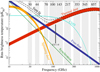Fig. 1. Illustration of the spectral energy density response of each component in the microwave emission. The shaded bands indicate the nine different observation frequencies of the Planck space observatory. Our goal is to create a map of each component in the sky; “CMB” emission, “Thermal dust” emission, and so on, after making assumptions about the spectral behaviour of each component such as we do in this figure. We model the spectral behaviour as slightly different in each pixel; hence it is indicated using bands rather than lines. Figure 2 adds further detail. This figure is reproduced directly from Planck Collaboration X (2015).

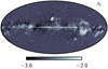Fig. 2. Example spectral index map $\beta (\widehat{n})$. Each pixel value corresponds to the slope in Fig. 1 in that pixel for a single combined low-frequency emission component (using a single component to represent the “Free-free”, “Synchrotron”, and “Spinning dust” emission types indicated in Fig. 1. In reality, each pixel is the sum of multiple slightly different spectral behaviours from different clouds of particles behind one another, but we instead work with a single compromise value for the dominating emission in the given direction. The mixing maps of this paper, $q_{\nu ,k}({\widehat{n}}_i)$, are taken to be proportional to ${\nu }^{\beta ({\widehat{n}}_i)}$, where each component k has a different β-map. This figure is reproduced directly from Planck Collaboration X (2015).

where $s_k(\widehat{n})$ represents the underlying component amplitude, and $q_{\nu ,k}(\widehat{n})$ represents an assumed mixing map. We will model the CMB component simply as another diffuse component, but note that the mixing maps are in that case spatially constant.

We do not observe $f_{\nu }(\widehat{n})$ directly, but rather take as input a pixelized sky map d_ν, where f_ν has been convolved with an instrumental beam and then further contaminated by instrumental noise. To simplify notation we employ a notation with stacked vectors, and write

$$\begin{array}{c}\hfill \mathit{d}\equiv \left[\begin{array}{c}{\mathit{d}}_{30\mathrm{GHz}}\\ {\mathit{d}}_{70\mathrm{GHz}}\\ ⋮\end{array}\right],\mathit{s}\equiv \left[\begin{array}{c}{\mathit{s}}_{\mathrm{cmb}}\\ {\mathit{s}}_{\mathrm{dust}}\\ ⋮\end{array}\right].\end{array}$$

Our data observation model can then be written

$$\begin{array}{c}\hfill \mathit{d}=\mathsf{P}\mathit{s}+\mathit{n},\end{array}$$(2)

where P is an N_obs × N_comp block-matrix where each block (ν, k) projects component s_k to the observed sky map d_ν, and n represents instrumental noise, and is partitioned in the same way as d. The noise n_ν is a pixelized map with the same resolution as d_ν, and assumed to be Gaussian distributed with zero mean. For our experiments we also assume that the noise is independent between pixels, so that Var(n_ν)≡N_ν is a diagonal matrix, although this is not a fundamental requirement of the method. We do, however, require that the matrix ${\mathsf{N}}_{\nu }^{-1}$ can somehow be efficiently applied to a vector.

Each component s_k represents the underlying, unconvolved field. In our implementation we work with s_k being defined by the spherical harmonic expansion of $s_k(\widehat{n})$, truncated at some band-limit L_k, that is, we assume s_ℓ, m = 0 for ℓ >  L_k. The choice of L_k is essentially a part of the model, and typically chosen to match a resolution that the observed sky maps will support. Additionally, each component s_k may have an associated Gaussian prior p(s), specified through its covariance matrix S. The role of the prior is to introduce an assumption on the smoothness of s. The prior typically does not come into play where the signal for a component is strong, but in regions that lack the component it serves to stabilize the solution, such that less noise is interpreted as signal. Computationally it is easier to assume the same smoothness prior everywhere on the sky, in which case the covariance matrix Var(s) = S is diagonal in spherical harmonic domain with elements given by the spherical harmonic power spectrum, C_k, ℓ. However, this is not a necessary assumption, and we comment on a different type of prior in Sect. 6.

The CMB power spectrum prior, given by C_cmb, ℓ, is particularly crucial. For the purposes of full sky component separation one would typically not specify any prior so as not to bias the CMB. For the purposes of estimating foregrounds, however, or filling in a CMB realization within a mask, one may insert a fiducial power spectrum predicted by some cosmological models.

We now return to the projection operator P, which projects each component to the sky. This may be written in the form of a block matrix with each column representing a component k and each row representing a sky observation ν, for example,

$$\begin{array}{c}\hfill \mathsf{P}=\left[\begin{array}{ccc}{\mathsf{P}}_{30\mathrm{GHz},\mathrm{cmb}}& {\mathsf{P}}_{30\mathrm{GHz},\mathrm{dust}}& \dots \\ {\mathsf{P}}_{70\mathrm{GHz},\mathrm{cmb}}& {\mathsf{P}}_{70\mathrm{GHz},\mathrm{dust}}& \dots \\ ⋮& ⋮& \ddots \end{array}\right],\end{array}$$(3)

with each block taking the form

$$\begin{array}{c}\hfill {\mathsf{P}}_{\nu ,k}={\mathsf{Y}}_{\nu }{\mathsf{B}}_{\nu }{\stackrel{\sim }{\mathsf{Q}}}_{\nu ,k}.\end{array}$$(4)

The operator Y_ν denotes spherical harmonic synthesis to the pixel grid employed by d_ν. We assume in this paper an azimuthally symmetric instrumental beam for each sky map, in which case the beam convolution operator B_ν is diagonal in spherical harmonic domain with elements b_ν, ℓ. This transfer function decays to zero as ℓ grows at a rate that fits the band-limit of the grid. Finally ${\stackrel{\sim }{\mathsf{Q}}}_{\nu ,k}$ is an operator that denotes point-wise multiplication of the input with the mixing map $q_{\nu ,k}(\widehat{n})$; computationally this should be done in pixel domain, so that

$$\begin{array}{c}\hfill {\stackrel{\sim }{\mathsf{Q}}}_{\nu ,k}={\mathsf{Y}}_{\nu ,k}^T{\mathsf{W}}_{\nu ,k}{\mathsf{Q}}_{\nu ,k}{\mathsf{Y}}_{\nu ,k},\end{array}$$(5)

where Q_ν, k contains $q_{\nu ,k}(\widehat{n})$ on its diagonal. The subscripts on the SHT operators indicate that these are defined on a grid specific to this mixing operation. We note that ${\stackrel{\sim }{\mathsf{Q}}}_{\nu ,k}$ will cause the creation of new small-scale modes, implying that, technically speaking, the band-limit of ${\stackrel{\sim }{\mathsf{Q}}}_{\nu ,k}{\mathit{s}}_k$ is 2L_k rather than L_k for a full-resolution mixing map q_ν, k. For typical practical system solving, however, the mixing matrices are usually smoother than the corresponding amplitude maps (due to lower effective signal-to-noise ratios), and the model may incorporate an approximation in that ${\stackrel{\sim }{\mathsf{Q}}}_{\nu ,k}$ truncates the operator output at some lower band-limit. At any rate, the grid used for Q_ν, k should accurately represent q_ν, k up to this band-limit. For this purpose it is numerically more accurate to use a Gauss-Legendre grid, rather than the HEALPix¹ grid (Górski et al. 2005) that is usually used for d_ν. The solver of the present paper simply treats this as a modelling detail, and any reasonable implementation works fine as long as ${\stackrel{\sim }{\mathsf{Q}}}_{\nu ,k}$ is not singular. However, to achieve reasonable efficiency, we do require $q_{\nu ,k}(\widehat{n})$ to be relatively flat, such that approximating ${\stackrel{\sim }{\mathsf{Q}}}_{\nu ,k}$ with a simple scalar q_ν, k is a meaningful zero-order representation. In practice we typically find ratios between the maximum and minimum values of $q_{\nu ,k}(\widehat{n})$ of 1.5–3. In general, the higher the contrast, the slower is the convergence of the solver.

2.3. Constrained realization linear system

We have specified a model for the components s where the likelihood p(d) and component priors p(s) are Gaussian, and so the Bayesian posterior is also Gaussian (Jewell et al. 2004; Wandelt et al. 2004; Eriksen et al. 2004b, 2008), and given by

$$\begin{array}{c}\hfill p(\mathit{s}|\mathit{d},\mathsf{S})\propto {\mathrm{e}}^{-\frac{1}{2}{\mathit{s}}^T{({\mathsf{S}}^{-1}+{\mathsf{P}}^T{\mathsf{N}}^{-1}\mathsf{P})}^{-1}\mathit{s}}.\end{array}$$(6)

To explore this density we are typically interested in either i) the mean vector, or ii) drawing samples from the density. Both can be computed by solving a linear system Ax = b with

$$\begin{array}{c}\hfill \mathsf{A}\equiv {\mathsf{S}}^{-1}+{\mathsf{P}}^T{\mathsf{N}}^{-1}\mathsf{P}\end{array}$$(7)

and

$$\begin{array}{c}\hfill \mathit{b}\equiv {\mathsf{P}}^T{\mathsf{N}}^{-1}\mathit{d}+{\mathsf{P}}^T{\mathsf{N}}^{-1/2}{\omega }_1+{\mathsf{S}}^{-1/2}{\omega }_2.\end{array}$$(8)

The vectors ω₁ and ω₂ should either be

• (i)

  zero, in which case the solution x will be the mean E(s|d, S), also known as the Wiener-filtered map; or

• (ii)

  vectors of variates from the standard Gaussian distribution, in which case the solution x will be samples drawn p(s|d, S). We refer to such samples as the constrained realizations.

For convenience we refer to the system as the constrained realization (CR) system in both cases. The computation of the right-hand side b is straightforward and not discussed further in this paper; our concern is the efficient solution of the linear system Ax = b.

For current and future CMB experiments, the matrix A is far too large for the application of dense linear algebra. However, we are able to efficiently apply the matrix to a vector, by applying the operators one after the other, and so we can use iterative solvers for linear systems. Since A is symmetric and positive definite, the recommended iterative solver is the conjugate gradients (CG) method (see Shewchuk 1994, for a tutorial). One starts with an arbitrary guess, say, x₁ = 0. Then, for each iteration, a residual r_i = b − Ax_i is computed, and then this residual is used to produce an updated iterate x_i + 1 that lies closer to the true solution x_true.

The residual r_i, which is readily available, is used as a proxy for the error, e_i = x_true − x_i, which is unavailable as we do not know x_true. The key is that since Ax_true = b,

$$\begin{array}{c}\hfill {\mathit{r}}_i=\mathit{b}-\mathsf{A}{\mathit{x}}_i=\mathsf{A}({\mathit{x}}_{}\text{true}-{\mathit{x}}_i)=\mathsf{A}{\mathit{e}}_i,\end{array}$$

and since A is linear, reducing the magnitude of r_i will also lead to a reduction in the error e_i. In a production run the error e_i is naturally unavailable, but during development and debugging it is highly recommended to track it. This can be done by generating an x_true, then generating b = Ax_true, and tracking the error e_i while running the solver on this input. The benchmark results presented in this paper are generated in this manner.

The number of iterations required by CG depends on how uniform (or clustered) the eigenspectrum of the matrix is. Therefore the main ingredient in a linear solver is a good preconditioner that improves the eigenspectrum. A good preconditioner is a symmetric, positive definite matrix M such that Mx can be quickly computed, and where the eigenspectrum of MA is as flat as possible, or at least clustered around a few values. Intuitively, M should in some sense approximate A⁻¹.

3. Full sky preconditioner based on pseudo-inverses

3.1. Pseudo-inverses

The inspiration for the solver presented below derives from the literature on the numerical solution of saddle-point systems. Our system A, in the form given in Eq. (7), is an instance of a so-called Schur complement, and approximating the inverse of such Schur complements plays a part in most solvers for saddle-point systems. An excellent review on the solution of saddle-point systems is given in Benzi et al. (2005). The technique we will use was originally employed by Elman (1999) and Elman et al. (2006), who use appropriately scaled pseudo-inverses to develop solvers for Navier-Stokes partial differential equations.

The pseudo-inverse is a generalization of matrix inverses to rectangular and/or singular matrices. In our case, we will deal with an m × n-matrix U with linearly independent columns and m >  n, in which case the pseudo-inverse is given by

$$\begin{array}{c}\hfill {\mathsf{U}}^{+}\equiv {({\mathsf{U}}^T\mathsf{U})}^{-1}{\mathsf{U}}^T.\end{array}$$

We note that in this case, U⁺ is simply the matrix that finds the least-squares solution to the linear system Ux = b, i.e., that minimizes min_x||Ux − b||². This matrix has the property that

$$\begin{array}{c}\hfill {\mathsf{U}}^{+}\mathsf{U}={({\mathsf{U}}^T\mathsf{U})}^{-1}{\mathsf{U}}^T\mathsf{U}=\mathsf{I},\end{array}$$

and so it is a left inverse. Unlike the real inverse however, UU⁺ ≠ I. This follows from U⁺ having the same shape as U^T, so that UU⁺ is necessarily a singular matrix. For small matrices, U⁺ can be computed by using the QR-decomposition. In the case that U does not have full rank, the pseudo-inverse has a different definition and should be computed using the singular value decomposition (SVD); the definition above is, however, sufficient for our purposes.

3.2. Full-sky, single component, without prior

For the first building block of our preconditioner we start with a much simpler linear problem. Assuming a model with a single sky map d, a single component, no mixing maps, and no prior, the linear system of Eq. (7) simply becomes

$$\begin{array}{c}\hfill \mathsf{B}{\mathsf{Y}}^T{\mathsf{N}}^{-1}\mathsf{Y}\mathsf{B}\mathit{x}=\mathit{b}.\end{array}$$(9)

We note that Y^T is not the same as spherical harmonic analysis, which in our notation reads Y^TW. Without the weight matrix W, Y^T represents adjoint spherical harmonic synthesis, and simply falls out algebraically from the transpose sky projection P^T.

Since the basis of x is in spherical harmonic domain, the beam convolution operator B is diagonal and trivially inverted. The remaining matrix Y^TN⁻¹Y is diagonal in pixel domain, so if only Y had been invertible we could have solved the system directly. Inspired by Elman (1999), we simply pretend that Y is square, and let Y^TW play the role of the inverse, so that

$$\begin{array}{c}\hfill {(\mathsf{B}{\mathsf{Y}}^T{\mathsf{N}}^{-1}\mathsf{Y}\mathsf{B})}^{-1}\approx {\mathsf{B}}^{-1}{\mathsf{Y}}^T\mathsf{W}\mathsf{N}\mathsf{W}\mathsf{Y}{\mathsf{B}}^{-1}.\end{array}$$(10)

We stress that because Y is not exactly invertible and Y^TW is a pseudo-inverse, this is only an approximation that should be used as a preconditioner inside an iterative solver. For the HEALPix grid in particular, Y^TW is rather inaccurate and we only have Y^TWY ≈ I; it is, however, a very good approximation, as can be seen in Fig. 3.

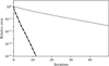Fig. 3. Convergence of preconditioner of Eq. (10) (black circles) compared to a simple diagonal preconditioner (grey ticks). In this case, we fit a single CMB component to a single 143 GHz Planck band without specifying a prior. Section 5 gives further details on the benchmark setup and the diagonal preconditioner.

3.3. Full sky, multiple components, with priors

Next, we want to repeat the above trick for a case with multiple sky maps d_ν, multiple components x_k, and a prior. We start by assuming that the mixing operators ${\stackrel{\sim }{\mathsf{Q}}}_{\nu ,k}$ can be reasonably approximated by a constant,

$$\begin{array}{c}\hfill {\stackrel{\sim }{\mathsf{Q}}}_{\nu ,k}\approx q_{\nu ,k}\mathsf{I},\end{array}$$

although, as noted above, this is only a matter of computational efficiency of the preconditioner. The optimal value for q_ν, k is given in Appendix A.2. In the following derivation we will simply assume equality in this statement, keeping in mind that all the manipulations only apply to the preconditioner part of the CG search, and so do not affect the computed solution.

First we note that the matrix of Eq. (7) can be written

$$\begin{array}{c}\hfill \mathsf{A}=\left[\begin{array}{cc}{\mathsf{P}}^T& \mathsf{I}\end{array}\right]\left[\begin{array}{cc}{\mathsf{N}}^{-1}& \\ & {\mathsf{S}}^{-1}\end{array}\right]\left[\begin{array}{c}\mathsf{P}\\ \mathsf{I}\end{array}\right].\end{array}$$

Writing the system in this way makes it evident that in the Bayesian framework, the priors are treated just like another “observation” of the components. These “prior observations” play a bigger role for parts of the solution where the instrumental noise is high, and a smaller role where the instrumental noise is low (see Fig. 4).

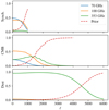Fig. 4. Visualization of the matrix U in an example setup. For each component k we plot the coefficients along the corresponding column of U, normalized so that the sum is 1 for each ℓ. We note how the CMB has most support from the 100 GHz band for low ℓ, then gradually switches to the 353 GHz band and finally the prior as ℓ increases.

The idea is now to further rearrange and re-scale the system in such a way that all information that is not spatially variant is expressed in the projection matrix on the side, leaving a unit-free matrix containing only spatial variations in the middle. Since S⁻¹ is assumed to be diagonal, it is trivial to factor it and leave only the identity in the centre matrix. Turning to the inverse-noise term N⁻¹, we find experimentally that re-scaling with a scalar performed well. Specifically, we define

$$\begin{array}{c}\hfill {\stackrel{\sim }{\mathsf{N}}}_{\nu }^{-1}\equiv {\alpha }_{\nu }^{-2}{\mathsf{Y}}_{\nu }^T{\mathsf{N}}_{\nu }^{-1}{\mathsf{Y}}_{\nu },\end{array}$$

where α takes the value that minimizes $\Vert {\stackrel{\sim }{\mathsf{N}}}_{\nu }^{-1}({\alpha }_{\nu }){-\mathsf{I}\Vert }_2$. Computing α_ν is cheap, and its optimal value is derived in Appendix A.1. A similar idea is used by Elsner & Wandelt (2013), as they split N⁻¹ into a spherical harmonic term and a pixel term, but their split is additive rather than multiplicative. Our system can now be written

$$\begin{array}{c}\hfill \mathsf{A}={\mathsf{U}}^T\mathsf{T}\mathsf{U},\end{array}$$(11)

where T contains the unit-free spatial structure of the system, and U the spatially invariant, but ℓ-dependent, structure of the system:

$$\begin{array}{c}\hfill \mathsf{T}\equiv \left[\begin{array}{cc}{\stackrel{\sim }{\mathsf{N}}}^{-1}& \\ & \mathsf{I}\end{array}\right],\mathsf{U}\equiv \left[\begin{array}{c}\alpha \mathsf{B}\stackrel{\sim }{\mathsf{Q}}\\ {\mathsf{S}}^{-1/2}\end{array}\right].\end{array}$$

In order to elucidate the block structure of these matrices, we write out an example with three bands and two components:

$$\begin{array}{c}\hfill \mathsf{T}=\left[\begin{array}{cccc}{\stackrel{\sim }{\mathsf{N}}}_1^{-1}& & & \\ & {\stackrel{\sim }{\mathsf{N}}}_2^{-1}& & \\ & & {\stackrel{\sim }{\mathsf{N}}}_3^{-1}& & \\ & & & \\ & & \mathsf{I}& \\ & & & \mathsf{I}\end{array}\right],\mathsf{U}=\left[\begin{array}{cc}{\alpha }_1{\mathsf{B}}_1{\stackrel{\sim }{\mathsf{Q}}}_{1,1}& {\alpha }_1{\mathsf{B}}_1{\stackrel{\sim }{\mathsf{Q}}}_{1,2}\\ {\alpha }_2{\mathsf{B}}_2{\stackrel{\sim }{\mathsf{Q}}}_{2,1}& {\alpha }_2{\mathsf{B}}_2{\stackrel{\sim }{\mathsf{Q}}}_{2,2}\\ {\alpha }_3{\mathsf{B}}_3{\stackrel{\sim }{\mathsf{Q}}}_{3,1}& {\alpha }_3{\mathsf{B}}_3{\stackrel{\sim }{\mathsf{Q}}}_{3,2}\\ {\mathsf{S}}_1^{-1/2}& \\ & {\mathsf{S}}_2^{-1/2}\end{array}\right].\end{array}$$

Under the assumption that ${\stackrel{\sim }{\mathsf{Q}}}_{\nu ,k}=q_{\nu ,k}\mathsf{I}$, the matrix U is block-diagonal with small blocks of variable size when seen in ℓ- and m-major ordering. Specifically, the entries in the “data-blocks” (ν, k′) in the top part of U are given by

$$\begin{array}{c}\hfill U_{(\ell ,m,\nu ),(\ell \prime ,m\prime ,k\prime )}={\alpha }_{\nu }{b}_{\nu ,\ell }{q}_{\nu ,k\prime }{\delta }_{\ell ,\ell \prime }{\delta }_{m,m\prime },\end{array}$$(12)

and the entries in the “prior-blocks” (k, k′) in the bottom part of U are given by

$$\begin{array}{c}\hfill U_{(\ell ,m,k),(\ell \prime ,m\prime ,k\prime )}=C_{k,\ell }^{-1/2}{\delta }_{k,k\prime }{\delta }_{\ell ,\ell \prime }{\delta }_{m,m\prime }.\end{array}$$(13)

In the event that no prior is present for a component, the corresponding block can simply be removed from the system, or one may equivalently set $C_{k,\ell }^{-1/2}=0$.

At this point we must consider the multi-resolution nature of our setup. Our model assumes a band-limit L_k for each component, so that each component has (L_k + 1)² corresponding columns in U, and, if a prior is used, an additional corresponding (L_k + 1)² rows. Each sky observation has a natural band-limit L_ν where the beam transfer function b_ν, ℓ has decayed so much that including further modes is numerically irrelevant, and so each band has (L_ν + 1)² corresponding rows in U. When we view U in the block-diagonal ℓ- and m-major ordering, the block sizes are thus variable. Each band-row only participates for ℓ ≤ L_ν, and each component-column and component-row only participates for ℓ ≤ L_k. A way to see this is to consider that the first blocks for ℓ = 0 have size (N_obs + N_comp)×N_comp for all m; then, as ℓ is increased past some L_ν or L_k, corresponding rows or columns disappear from the blocks.

In code it is easier to introduce appropriate zero-padding for ℓ >  L_k and ℓ >  L_ν so that one can work with a single constant block size. Either way, the numerical results are equivalent. Since U consists of many small blocks on the diagonal, computing the pseudo-inverse is quick, and the memory use and compute time for constructing U⁺ scales as $O(N_{\text{comp}}{}^2{N}_{\text{obs}}{L}^2)$.

With this efficient representation of U⁺ in our toolbox, we again use the trick of Elman (1999) to construct a preconditioner in the form

$$\begin{array}{c}\hfill {\mathsf{A}}^{-1}={({\mathsf{U}}^T\mathsf{T}\mathsf{U})}^{-1}\approx {\mathsf{U}}^{+}{\mathsf{T}}^{-1}{({\mathsf{U}}^{+})}^T.\end{array}$$(14)

The lower right identity blocks of T require no inversion. The ${\stackrel{\sim }{\mathsf{N}}}_{\nu }^{-1}$-blocks in the upper left section of T can be approximately inverted using the technique presented in Sect. 3.2, so that

$$\begin{array}{c}\hfill {({\stackrel{\sim }{\mathsf{N}}}_{\nu }^{-1})}^{-1}\approx {\alpha }_{\nu }^2{\mathsf{Y}}_{\nu }^T{\mathsf{W}}_{\nu }{\mathsf{N}}_{\nu }{\mathsf{W}}_{\nu }{\mathsf{Y}}_{\nu }.\end{array}$$

Let T⁺ denote T⁻¹ approximated in this manner, and the resulting preconditioner is

$$\begin{array}{c}\hfill {\mathsf{M}}_{}\text{PI}={\mathsf{U}}^{+}{\mathsf{T}}^{+}{({\mathsf{U}}^{+})}^T.\end{array}$$(15)

Computationally speaking, this has the optimal operational form: the pseudo-inverse U⁺ and its transpose can be applied simply by a series of small matrix-vector products in parallel using the pre-computed blocks, while application of T⁺ as an operator requires 2N_obs SHTs.

So far we have only considered the pseudo-inverse as an algebraic trick, but some analytic insights are also available. First we look at two special cases. The preconditioned system can be written

$$\begin{array}{c}\hfill {\mathsf{M}}_{}\text{PI}\mathsf{A}={({\mathsf{U}}^T\mathsf{U})}^{-1}{\mathsf{U}}^T{\mathsf{T}}^{+}\mathsf{U}{({\mathsf{U}}^T\mathsf{U})}^{-1}{\mathsf{U}}^T\mathsf{T}\mathsf{U}.\end{array}$$

First, we note that if the real model indeed has a flat inverse-noise variance map, then T⁺ = T = I and the preconditioner is perfect, MA = I. Second, we consider the case in which the inverse-noise variance maps are not flat, but that rather (1) N_comp = N_obs; (2) there are no priors; and (3) the band-limit of each sky observation matches that of its dominating component. In this case, U is square and invertible, and (U^TU)⁻¹U^T = U⁻¹, and thus MA = U⁻¹T⁺TU ≈ I, using the very good approximation developed in Sect. 3.2.

In the generic case, T ≠ I, and U has more rows than columns. First we note that for an other equivalent model with constant inverse-noise variance maps, the corresponding system matrix is A_F ≡ U^TU. Further, we can define a system that acts just like A in terms of effects that are spatially invariant, but which has the inverse effect when it comes to the scale-free spatial variations: A_SPI ≡ U^TT⁺U. With these definitions we have

$$\begin{array}{cc}\hfill {\mathsf{M}}_{}\text{PI}\mathsf{A}& ={\mathsf{A}}_{}^{-1}\text{F}{\mathsf{A}}_{}\text{SPI}{\mathsf{A}}_{}^{-1}\text{F}\mathsf{A}.\hfill \end{array}$$

The operator above applies the spatially variant effects once forward and once inversely, and the spatially invariant effects twice forward and twice inversely. Everything that is done is also undone, and in this sense M_PIA can be said to approximate I.

To see where the approximation breaks down, one must consider what A_SPI actually represents, which is a linear combination of the spatial inverses of the inverse-noise maps and the priors. The U matrix gives more weight to a band with more information for each component. For instance, in a Planck-type setup that includes a thermal dust component, the spatial inverse of the 857 GHz band will be given strong weight, while the spatial inverse of 30 GHz will be entirely neglected, as desired. Likewise, the prior terms will be given little weight in the data-dominated regime at low multipoles, and then gradually be introduced as the data becomes noise dominated.

However, the weights between the spatial inverses ignore spatial variations, and only account for the average within each multipole ℓ. Thus the preconditioner only works well when faced with modest spatial variations in the inverse-noise maps. This is illustrated in Fig. 5. For the spatially invariant part of the preconditioner, the crossover between the inverse-noise dominated regime and the prior-dominated regime must happen at a single point in ℓ-space, whereas in reality this point varies based on spatial position for ℓ in the mid-range where the prior lines are crossing the inverse-noise bands.

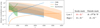Fig. 5. Left panel: relative amplitudes of the prior term (solid lines; ${\mathsf{S}}_k^{-1}$) and inverse-noise term (diffuse bands; $\sum _{\nu }{\mathsf{P}}_{\nu ,k}^T{\mathsf{N}}_{\nu }^{-1}{\mathsf{P}}_{\nu ,k}$) on the diagonal of the coefficient matrix A. Each full inverse-noise band has been evaluated by summing over the nine Planck frequency bands. The darker part of each band displays the extents of the inverse-noise terms if one reduces contrast by adding synthetic regularization noise to the 1% least noisy pixels. This in turn reduces the condition number of the full matrix. Where the solid lines lie above the diffuse bands, the full matrix is prior dominated; where they lie below, the full matrix is data dominated. Right panel: schematic setup of which term dominates A in different regimes. The pseudo-inverse preconditioner of Sect. 3 automatically resolves the low-ℓ versus high-ℓ split, taking into account cross-component couplings. To handle the crucial low-ℓ regime inside the mask (red), the extension described in Sect. 4 is required.

Figure 6 summarizes the performance of the above preconditioner in a realistic full sky component separation setup in terms of iteration count. The analysis set-up corresponds to a standard nine-band Planck data set in terms of instrumental noise levels and beam characteristics, as most recently reported by Planck Collaboration IV (2019).

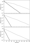Fig. 6. Convergence of the pseudo-inverse preconditioner (shown in black lines) for a full-sky component separation model for three different sets of mixing matrices with varying spatial structure. For comparison, grey lines show the convergence of a block diagonal preconditioner. The top panel shows a case with full-resolution mixing matrices; the middle panel shows a case with mixing matrices smoothed to 20′ and 1° FWHM for thermal dust and synchrotron emission, respectively; and the bottom panel shows a case with spatially uniform mixing matrices. Further details are given in Sect. 3.3.

1. Synchrotron with a band-limit of L_synch = 1000, a Gaussian prior C_synch, ℓ with FWHM of 30 arc-minutes, and with signal-to-noise ratio of unity at ℓ = 350.

2. CMB with a band-limit of L_cmb = 4000, a ΛCDM power spectrum prior, and with signal-to-noise ratio of unity around ℓ = 1600.

3. Thermal dust with a band-limit L_dust = 6000 and a signal-to-noise ratio of unity around ℓ = 4500.

All mixing matrices are adopted from the Commander temperature analysis described by Planck Collaboration IV (2019), which accounts for full spatial variations in both the synchrotron² and thermal dust components.

In the top panel we show a model for which the full-resolution high-contrast mixing maps are retained for both the dust and synchrotron components. The spatial variations in the mixing maps $q_{\nu ,k}(\widehat{n})$ are not modelled in the preconditioner, and so both preconditioners struggle in this case, but the pseudo-inverse preconditioner is still twice as fast as the block-diagonal preconditioner. In the middle panel, we apply a Gaussian low-pass filter to the mixing maps, reducing both local spatial variation and contrast. We applied Gaussian filters with a FWHM of 20 arc-minutes for the dust component and 1° for the synchrotron component. This improves the convergence rate by about a factor of two. Finally, in the bottom panel the mixing maps have no spatial variation at all, and the entire foreground model is described by the preconditioner. This represents the limiting optimal case for this particular setup.

The pseudo-inverse preconditioner is at a greater advantage in situations with moderate structure and contrasts in the mixing maps. Unlike the diagonal preconditioner, the pseudo-inverse preconditioner solves for the structure in the inverse-noise matrix N⁻¹, but neither solves for the spatial structure in mixing maps. On a harder problem in general, it seems that diagonal preconditioner is put at a (relative) advantage by having more iterations at which to also work on the inverse-noise term.

It should be noted that the pseudo-inverse preconditioner requires extra SHTs compared to a standard diagonal preconditioner, and so requires more computing time per iteration. This penalty is highly model specific as it depends on N_comp and N_obs. In general, each multiplication with A requires (2N_comp + 4N_obs), which translates into 42 SHTs for our case, whereas application of the pseudo-inverse preconditioner requires 2N_obs = 18 SHTs. Additional optimizations can be made if one or more mixing matrices are spatially uniform, as for instance is the case for the CMB component. If all components have the same resolution, this translates to each iteration of the pseudo-inverse solver taking about 33% longer than the block-diagonal preconditioner, and with a third of the iterations needed, we end up with a total run-time reduction of 60%. For this model, the synchroton with a flat mixing map has much lower angular resolution than the dust component with a variable mixing map, and so the speed-up is somewhat larger. In the future it could be possible to use approximate SHTs to significantly reduce this overhead (see Sect. 6).

4. Constrained realization under a mask

So far we have only considered the full sky case. In many practical applications, we additionally want to mask out parts of the sky, either because of missing data, or because we do not trust our model in a given region of the sky. Within such scenarios, it is useful to distinguish between two very different cases:

• (i)

  Partial sky coverage, where only a small patch of the sky has been observed, and we wish to perform component separation only within this patch. The typical use case for this setup is ground-based or sub-orbital CMB experiments.

• (ii)

  Natively full sky coverage, but too high foregrounds in a given part of the sky to trust our model. In this case, one often masks out part of the sky, but still seeks a solution to the system under the mask, constrained by the observed sky at the edges of the mask and determined by the prior inside the mask. By ignoring data from this region we at least avoid the CMB component being contaminated by foreground emission. Of course, the solution will not be the true CMB sky either, but it will have statistically correct properties for use inside of a Gibbs sampler (Jewell et al. 2004; Wandelt et al. 2004; Eriksen et al. 2004b, 2008).

We expect the solver developed in the previous section to work well in case (i) given appropriate modifications, but leave such modifications for future work, and focus solely on case (ii) in what follows.

4.1. Incorporating a mask in the model while avoiding ringing effects

We recall from Sect. 2.2 that our data model reads

$$\begin{array}{c}\hfill \mathit{d}={\mathsf{Y}}_{\nu }{\mathsf{B}}_{\nu }{\stackrel{\sim }{\mathsf{Q}}}_{\nu ,k}\mathit{s}+\mathit{n},\end{array}$$

where d are the pixels of the observed sky maps. We follow Eriksen et al. (2004b) and Seljebotn et al. (2014) and introduce a mask in the model by declaring that the masked-out pixels are missing from d, or, equivalently, that N⁻¹ is zero in these pixels. This is straightforward from a modelling perspective, but has an inconvenient numerical problem: ideally, we want to specify the beam operator B using a spherical harmonic transfer function b_ℓ, but, because b_ℓ must necessarily be band-limited, B exhibits ringing in its tails in pixel basis. Specifically, in pixel space the beam operator first exhibits an exponential decay, as desired, but then suddenly stops decaying before it hits zero. At this point, it starts to observe the entire sky through the ringing “floor” (see figures in Seljebotn et al. 2014), and it becomes non-local. When the signal-to-noise ratio of the data in question is high enough compared to such numerical effects, the model will try to predict the signal component s within the mask through deconvolution of the pixels at the edge of the mask, regardless of their distance. This causes a major complication for all solvers of this type, and in Seljebotn et al. (2014) we had to carefully tune the solver to avoid this ringing effect.

In the present solver we introduce the mask in the mixing maps Q_ν, k, rather than in the noise model, but only in the preconditioner. This corresponds to making the approximation that beam convolution and masking commute, even though these operations do in fact not commute. The sky is then split cleanly into one set of pixels outside the mask that hits the full matrix S⁻¹ + P^TN⁻¹P, and another set of pixels (those under the mask) that only hits the prior term S⁻¹. We then proceed to apply separate preconditioners in the two regions. This simple approximation, although far from exact, is good enough to support good convergence for the final solver.

4.2. Independently solving for signals under a mask

Let us consider the schematic description of each regime in the right panel of Fig. 5. The pseudo-inverse preconditioner, which we will denote M_PI, automatically finds a good split per component for the low- and high-ℓ regimes, respectively, but is, in the same way as a block-diagonal preconditioner, blind to the different regimes inside and outside of the mask. As a result, it performs poorly for large scales inside the mask, that is, for multipoles lower than the point of unity signal-to-noise ratio shown in Fig. 7.

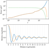Fig. 7. Harmonic filtering of the mask-restricted system ZS−1ZT. Top panel: inverse CMB power spectrum 1/Cℓ (solid blue), on the diagonal of the S−1 matrix behaves as ℓ2 near the beginning, increasing in steepness to ℓ8 at ℓ = 6000. It crosses the diagonal of the inverse-noise term N−1 (dotted green) at around ℓ = 1600. Above this point the system becomes prior dominated and the pseudo-inverse preconditioner works well both inside and outside the mask. Since we do not need the dedicated mask solver to solve for high ℓ, we apply a filter rℓ as described in Sect. 4.4, resulting in a filtered prior $r_{\mathcal{l}}^2/C_{\mathcal{l}}$ (dashed orange). Bottom panel: S−1 operator in pixel domain. The plot displays (YS−1YT)ij as a function of the distance between grid points i and j. Both the unfiltered operator 1/Cℓ (solid blue) and the low-pass filtered $r_{\mathcal{l}}^2/C_{\mathcal{l}}$ (dashed orange) have a “Mexican hat” or Wavelet-like azimuthally symmetric shape. The low-pass filter ensures that the oscillations decay quickly, making the system easier to solve in pixel domain than the unfiltered version.

To solve this, we supplement the pseudo-inverse preconditioner with a second preconditioner that is designed to work well only inside the mask, where it is possible to simplify the system. Let Z denote spherical harmonic synthesis to the pixels within the mask only; that is, we first apply Y, and then select only the masked pixels. Then, building on standard domain decomposition techniques, a preconditioner that provides a solution only within the masked region is given by

$$\begin{array}{c}\hfill {\mathsf{M}}_{}\text{mask}={\mathsf{Z}}^T{(\mathsf{Z}\mathsf{A}{\mathsf{Z}}^T)}^{-1}\mathsf{Z}={\mathsf{Z}}^T{(\mathsf{Z}{\mathsf{S}}^{-1}{\mathsf{Z}}^T)}^{-1}\mathsf{Z}.\end{array}$$(16)

We will develop a solver for the inner mask-restricted system in Sect. 4.4. The idea is then to use both the full-sky solver developed in Sect. 3.2 M_PI, and the mask-restricted solver M_mask. The simplest possible way of doing this is simply to add them together, M_add ≡ M_PI + M_mask, and we find experimentally that this simple combination performs well for our purposes. In our experiments we have chosen M_PI to simply be the unaltered full sky pseudo-inverse. As the full system matrix A does not in fact include values from the RMS map inside the mask, there is some freedom here to choose other values, although we found other choices to have little effect on overall convergence.

The preconditioner described above, however, may break down for more demanding models. We found that the most important feature in how well M_add works is how far the inverse-noise term decays before it is overtaken by the prior term (see Fig. 7). In the case of analysing Planck data, we find that the inverse-noise term decays by a factor of roughly λ = 0.15 at this point, which is unproblematic. In simulations with lower resolution or higher noise, such that λ = 0.01, convergence is hurt substantially, and at λ = 0.001 the preconditioner breaks down entirely.

Since our own use cases (which are targeted towards Planck) are not affected by this restriction, we have not investigated this issue very closely. We have, however, diagnosed the effect at low resolution with a dense system solver for (ZS⁻¹Z)⁻¹. In these studies, we find that the problem is intimately connected with how the two preconditioners are combined, and it may well be that more sophisticated methods for combining preconditioners will do a better job. For the interested reader, we recommend Tang et al. (2009) for an introduction to the problem, as they cover many related methods arising from different fields using a common terminology and notation. In particular it would be interesting to use deflation methods to “deflate” the mask subspace out of the solver. it will still be limited by the fundamental approximation in which we moved the mask from the inverse-noise term N⁻¹ to the mixing term Q, and this sets a limit to how well the preconditioner can work along the edges of the mask.

Finally, we give a word of warning: in the full sky case, we have been able to re-scale the CR system arbitrarily without affecting the essentials of the system. For instance, Eriksen et al. (2008) scale A with S^1/2 so that the system matrix becomes I + S^1/2P^TN⁻¹PS^1/2. This has no real effect on the spherical harmonic preconditioners, but in pixel domain it changes the shape of each term. The natural unscaled form of A is localized in pixel domain. The inverse-noise term essentially looks like a sum of the instrumental beams, while the prior defines smoothness couplings between a pixel and its immediate neighbourhood. However, S^1/2 is a highly non-local operator, and multiplying with this factor decreases locality and causes a break-down of our method. There may of course be other filters that would increase locality in pixel domain instead of decrease it, in which case it could be beneficial to apply them.

4.3. Including a low-pass filter in the mask-restriction

The feature that most strongly defines the mask-restricted system ZS⁻¹Z^T is the shape of the mask, and thus pixel basis is the natural domain in which to approach this system. The operator ZS⁻¹Z^T acts as a convolution with an azimuthally symmetric kernel on the pixels within the mask. In Fig. 7 we plot a cut through this convolution kernel (blue in bottom panel). Mainly due to the sharp truncation at the band-limit L, oscillations extend far away from the centre of the convolution kernel. To make the system easier to solve, we follow Seljebotn et al. (2014) and insert a low-pass filter as part of the restriction operator Z, so that the projection from spherical harmonics to the pixels within the mask is preceded by multiplication with the transfer function

$$\begin{array}{c}\hfill r_{\ell }=\text{exp}(-\beta {\ell }^2{(\ell +1)}^2),\end{array}$$(17)

where we choose β so that $r_{L/2}^2=0.05$. The resulting system now has a transfer function of $r_{\mathcal{l}}^2/C_{\mathcal{l}}$, whose associated convolution kernel is much more localized (dashed orange), making it easier to develop a good solver for ZS⁻¹Z^T.

After introducing this low-pass filter we no longer have equality in Eq. (16), but only approximately that ZAZ^T ≈ ZS⁻¹Z^T. This appears to not hurt the overall method, as r_ℓ is rather narrow when seen as a pixel-domain convolution (unlike $\sqrt{C_{\ell }}$, as noted above). Also we note that we have now over-pixelized the system ZS⁻¹Z, as higher frequency information has been suppressed and the core of the convolution kernel is supported by two pixels. Our attempts at representing ZS⁻¹Z on a coarser grid failed however, because the solution will not converge along the edge of the mask unless the grid of Z exactly matches the grid of the mixing map Q_ν, k. While the resulting system ZS⁻¹Z^T on the full-resolution grid is poorly conditioned for the smallest scales, this does not prevent us from applying iterative methods to solve for the larger scales.

4.4. Multi-grid solver for the mask-restricted system

Finally we turn our attention to constructing an approximate inverse for ZS⁻¹Z^T. We now write the same system matrix as

$$\begin{array}{c}\hfill \mathsf{G}=\mathsf{Z}{\mathsf{S}}^{-1}{\mathsf{Z}}^T=\mathsf{Y}\mathsf{D}{\mathsf{Y}}^T,\end{array}$$(18)

where D is a diagonal matrix with $d_{\mathcal{l}}=r_{\mathcal{l}}^2/C_{\mathcal{l}}$ on the diagonal, and it should be understood that the spherical harmonic synthesis Y only projects to grid points within the mask.

As noted in Seljebotn et al. (2014), in the case where d_ℓ ∝ ℓ² this is simply the Laplacian partial differential equation on the sphere, and the multi-grid techniques commonly used for solving this system are also effective in our case. We will focus on the case where C_ℓ is the CMB power spectrum; in this case 1/C_ℓ starts out proportional to ℓ², increasing to ℓ⁶ around ℓ ∼ 1600, eventually reaching ℓ⁸ at ℓ ∼ 6000. In theory this should make the system harder to solve than the Laplacian, but it seems that in our solver the application of the low-pass filter described in the previous section is able to work around this problem.

To solve the system Gx = b using iterative methods, we might start with a simple diagonal approximate inverse,

$$\begin{array}{c}\hfill \mathsf{M}\equiv \text{diag}{(\mathsf{G})}^{-1},\end{array}$$

which is in fact a constant scaling since G is spatially invariant. This turns out to work well as a preconditioner for the intermediate scales of the solution. For smaller scales (higher ℓ) the quickly decaying restriction r_ℓ starts to dominate over 1/C_ℓ such that the combined effect is that of a low-pass filter; such filters cannot to our knowledge be efficiently deconvolved in pixel domain and an harmonic-domain preconditioner would be required. Luckily, we do not need to solve for these smaller scales, as the pseudo-inverse preconditioner will find the correct solution in this regime, and the restriction operator Z will at any rate filter out whatever contribution comes from the solution of G.

The problem at larger scales (lower ℓ) is that the approximate inverse would have to embed inversion of the coupling of two distant pixels through a series of intermediate pixels in-between; this is beyond the reach of our simple diagonal preconditioner. For this reason we introduce a multi-grid (MG) V-cycle, where we recursively solve the system on coarser resolutions. For each coarsening, the preconditioner is able to see further on the sphere, as indirect couplings in the full-resolution system are turned into direct couplings in the coarser versions of the system. A basic introduction to multi-grid methods can be found for example in Hackbush (1985) or the overview given in Seljebotn et al. (2014).

The first ingredient in MG is an hierarchy of grids, which are denoted relatively, with h denoting an arbitrary level and H denoting the grid on the next coarser level. We have opted for a HEALPix grid for Q_ν, k and G, and use its hierarchical structure to define the coarser grid, simply letting N_side,H = N_side, h/2. We also need to consider which subset of grid points to include to represent the region within the mask. We got the best results by only including those pixels of H that are covered 100% by the mask in the fine grid h, so that no pixel on any level ever represents a region outside the full-resolution mask.

The second ingredient in MG is the restriction operator ${\mathsf{I}}_h^H$, which transfers a vector from grid h to grid H. We tried restriction operators both in pixel domain and spherical harmonic domain, and spherical harmonic restriction performed better by far. Thus we define

$$\begin{array}{c}\hfill {\mathsf{I}}_h^H={\mathsf{Y}}_H{\mathsf{R}}_H{\mathsf{Y}}_h^T{\mathsf{W}}_h,\end{array}$$(19)

where we use subscripts to indicate the grid of each operator, and where R_H has some harmonic low-pass filter r_H, ℓ on its diagonal. In Seljebotn et al. (2014) the corresponding filter had to be carefully tuned to avoid problems with ringing, because the N⁻¹-term created high contrasts in the system matrix. In the present method we no longer have to deal with the N⁻¹ term, and the requirements on the low-pass filter are much less severe, as long as they correspond to a convolution kernel with a FWHM of roughly one pixel on the coarse grid. A Gaussian band-limited at L_H = 3N_side,H = L_h/2 performed slightly better than the filter of Eq. (17) in our tests, even if it has somewhat more ringing at this band-limit.

The third ingredient in MG is the coarsened linear system

$$\begin{array}{c}\hfill {\mathsf{G}}_H={\mathsf{I}}_h^H{\mathsf{G}}_h{\mathsf{I}}_H^h={\mathsf{Y}}_H{\mathsf{D}}_H{\mathsf{Y}}_H^T,\end{array}$$(20)

where $d_{H,\mathcal{l}}=r_{H,\mathcal{l}}^2{d}_{h,\mathcal{l}}$ is band-limited at L_H = L_h/2³. We stress again that the grid H embeds the structure of the mask, so that Y_H in this context denotes spherical harmonic synthesis only to grid points within the mask. In computer code, zero padding is used outside of the mask before applying ${\mathsf{Y}}_H^T$, and entries outside the mask are discarded after applying Y_H.

The fourth ingredient in MG is an approximate inverse, in this context named the smoother. The name refers to removing small scales in the error x_true − x. Removing these scales happens through approximately solving the system, and should not be confused with applying a low-pass filter. In our case we will use the simple constant smoother M discussed above, although in combination with a damping factor ω = 0.2, so that the eigenvalues of ωMG are bounded above by 2 as required by the MG method. We write M_h = ω diag(G_h)⁻¹ for the smoother on level h.

Finally, the ingredients are combined in the simplest possible MG V-cycle algorithm (see Fig. 8). It turns out that the restriction and interpolation operations can share one SHT each with the associated system matrix multiplication, so that six SHTs are required per level. Furthermore, the SHTs can be performed at different resolutions for additional savings. Like the pseudo-inverse preconditioner, the mask-restricted solver appears to work well with approximate SHTs, enabling further savings in the future (see Sect. 6).

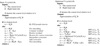Fig. 8. Pseudo-code for the MG V-cycle. The matrices involved are defined in the main text. Basic-V-Cycle: the clean textbook version, exposing the basic structure of the algorithm. The important feature of the algorithm is that the solution vector x is never transferred directly between levels. Instead, a residual rH is computed, which takes the role as the right-hand side b on the coarser level. The coarse solution is a correction cH that is then added to the solution vector x. The resulting full V-cycle is a symmetric linear operator that can be used as a preconditioner for CG. We keep recursing until there are less than 1000 coefficients left, and then solve using a pseudo-inverse based on the SVD, ${\mathsf{G}}_h^{+}\approx {\mathsf{G}}_h^{-1}$, as Gh may, depending on the size of the mask, be singular due to Dh being truncated at Lh. Optimized-V-Cycle: in this code we have inserted ${\mathsf{I}}_h^H={\mathsf{Y}}_H{\mathsf{R}}_H{\mathsf{Y}}_h^T{\mathsf{W}}_h$ and ${\mathsf{G}}_h={\mathsf{Y}}_h{\mathsf{D}}_h{\mathsf{Y}}_h^T$, and then reorganized the expressions so that the restriction and interpolation steps each share one SHT with the corresponding application of Gh. The J operator denotes ${\mathsf{Y}}_h^T{\mathsf{W}}_h{\mathsf{Y}}_h$. The effect of this operator is to zero out any contribution that falls outside of the mask in the (full sky) spherical harmonic vectors; but numerical experiments indicate that the term can in practice be neglected also when using a small mask. In our numerical experiments we approximate J ≈ I, reducing the total number of SHTs to six per level. The comments indicate the required resolution for each SHT, with Lh (LH) referring to fine (coarse) harmonic band-limit, and Nh (NH) referring to fine (coarse) grid.

Figure 9 shows the results of solving the full system when inserting this algorithm as an approximation of (ZS⁻¹Z^T)⁻¹ in Eq. (16). While the diagonal preconditioner degrades, M_add converges very quickly. The pseudo-inverse preconditioner M_PI by itself shows much the same behaviour as the diagonal preconditioner in this situation (not plotted).

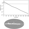Fig. 9. Convergence of the Madd preconditioner (top panel) when including sky mask (Planck Collaboration XI 2016) in the model (bottom panel). We fit a single CMB component to hypothetical foreground-cleaned maps on all nine Planck bands, specifying a fiducial Cℓ prior for the CMB power spectrum. We plot the convergence when using a diagonal preconditioner (grey) and the Madd preconditioner developed in Sect. 4 (black). Section 5 gives details on the benchmark setup.

5. Benchmark notes

The implementation used for the convergence plots in this paper are produced using a prototype implementation written in a mixture of Fortran, Cython, and Python, and is available under an open source license⁴. As a prototype, it does not support polarization or distributed computing with the Message Passing Interface (MPI). A full implementation in the production quality Commander code is in progress.

Simulations are performed with a known x_true drawn randomly from a Gaussian distribution, and a right-hand side given by b = Ax_true. Then the convergence statistic denoted “relative error” in these figures simply reads

$$\begin{array}{c}\hfill e_i\equiv \Vert {\mathit{x}}_i-{\mathit{x}}_{}\text{true}\Vert .\end{array}$$

Finally, unless otherwise noted, we add regularization noise to the 1% of the highest signal-to-noise pixels in the RMS maps. As noted in Fig. 3, this is more of an advantage for the diagonal preconditioner than the pseudo-inverse preconditioner, but this typically mimics what one would do in real analysis cases.

In the present paper we have focused strictly on algorithm development, and as such the prototype code is not optimized; we have not invested the effort to benchmark the preconditioners in terms of CPU time spent. As detailed in Sects. 3.3 and 4.4, the additional cost for a particular use case can be calculated from the number of extra SHTs.

The block-diagonal preconditioner we use as a comparison point is described in further detail by Eriksen et al. (2004b). In the notation of this paper, it can be written

$$\begin{array}{c}\hfill {\mathsf{M}}_{}\text{diag}\equiv {({\mathsf{U}}^T\text{diag}(\mathsf{T})\mathsf{U})}^{-1},\end{array}$$

where each element of diag(T) can be computed in O(L) time by a combination of Fourier transforms and computing the associated Legendre polynomials, which is available for example in the latest version of Libsharp⁵. Since the matrix U^Tdiag(T)U consists of (ℓ_max + 1)² blocks of size N_comp × N_comp, the inversion is cheap.

For the component separation case we provide three benchmarks in Fig. 7, with varying degrees of difficulty introduced through the mixing maps. For the benchmark of Fig. 9, we only included the CMB component, and so only a flat mixing map was in use.

6. Discussion and outlook

In this paper we have presented a versatile Bayesian model for the multi-resolution CMB component separation and constrained realization problem, as well as an efficient solver for the associated linear system. This model is currently in active use for component separation for the Planck 2017 collaboration. The final result is the ability to perform exact, full-resolution, multi-resolution component separation of full-sky microwave data within a reasonable number of conjugate gradient iterations.

To achieve such good convergence several novel techniques were employed. First, we developed a novel pseudo-inverse based preconditioner. For the full sky case this provides a speed-up of parameters. Second, we extended the model with a mask through the mixing maps, rather than through the noise covariance matrix, to avoid ringing problems associated with going between spherical harmonic domain and pixel domain. Third, we solved for the solution under the mask using a dedicated multi-grid solver in pixel domain restricted to the area under mask, where the linear system can be simplified.

We note that the pseudo-inverse preconditioner not only performs very well for the full sky case with reasonably uniform mixing maps, but it is also very simple to implement, significantly simpler than the previously standard diagonal preconditioner. As mentioned earlier, this technique is of course not novel for or restricted to CMB component separation; it has been in use for solving Navier-Stokes equations for some time. The fundamental idea is to approximate the total inverse of a sum with the best linear combination of inverses of each term. A problem related to this paper, which in particular fits this description, is the basic CMB map-making equation (e.g., Tegmark 1997). This equation is a sum over individual time segments of observations, which can in isolation be inverted in Fourier domain. If the pseudo-inverse preconditioner works well in this case, as we believe it will, it may speed up exact maximum likelihood map makers substantially.

Regarding more direct extensions of the work in the present paper, a natural next step is the use of a pixel domain basis instead of spherical harmonic coefficients to represent the microwave components. We have so far assumed an isotropic prior for all components that can be specified in the form of a power spectrum C_ℓ, with a sharp band-limit L. This model has a tendency to excite ringing in the resulting maps around sharp objects, unless much time is spent tuning the priors, or one adopts a very high band-limit L for all components. Working with pixel-domain vectors and, with the exception of the CMB, pixel-domain prior specifications, one could easily define the models that are more robust against this problem. Also, we know that the diffuse foregrounds have much variation where their signal is strong, but should be more heavily stabilized where their signal is weak. Such a non-isotropic prior is easier to model using a sparse matrix in pixel domain. Of particular interest are the so-called conditional auto-regressive (CAR) models, which have a natural interpretation and which directly produce sparse inverses S⁻¹.

Several SHT algorithms have been developed with a computational scaling of O(L² log L) or O(L²(log L)²). These are generally not used within the astrophysical community because of the large pre-factors involved and lack of optimized implementations. Some of these algorithms (e.g., Tygert 2008, 2010; Seljebotn 2012) can produce low-accuracy results at a much lower cost, since their pre-factor includes a term O(d²) with d representing the number of digits in the computation. As shown in Fig. 10, the preconditioner developed in this paper works well with approximate SHTs, and optimized implementations of these algorithms may speed up the preconditioner to the point where its computational cost is negligible compared to the matrix-vector multiplication.

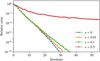Fig. 10. Effect of employing approximate SHTs in the preconditioner. To simulate approximate SHTs, for every SHT computer, we have multiplied each coefficient of the result with a random variate drawn uniformly from the interval [1 − ϵ, 1 + ϵ], simulating numerical noise at the ϵ-level. Note that we carried out these simulations on a resolution of Nside = 128, using the downgrade procedure outlined in Appendix C. The experiment is otherwise identical to the one in Fig. 9. The approximate SHTs are employed both in the pseudo-inverse preconditioner and the mask-restricted multi-grid solver, while the (non-preconditioner) matrix-vector multiplication uses the full accuracy provided by Libsharp.

Acknowledgments

We thank Jeff Jewell, Sigurd Næss, Martin Reinecke, and Mikolaj Szydlarski for useful input. This work was supported by European Research Council grants StG2010-257080 and CoG2017-772253, and the H2020 COMPET-4 grant 776282. Some of the results in this paper have been derived using the HEALPix (Górski et al. 2005), Libsharp (Reinecke & Seljebotn 2013), Healpy, NumPy, and SciPy software packages.

References

Appendix A: Details of the pseudo-inverse preconditioner

A.1. Approximating the inverse-noise maps

We seek α_ν such that the distance between ${\stackrel{\sim }{\mathsf{N}}}_{\nu }^{-1}$ and the identity matrix is minimized:

$$\begin{array}{cc}\hfill \Vert {\stackrel{\sim }{\mathsf{N}}}_{\nu }^{-1}({\alpha }_{\nu }){-\mathsf{I}\Vert }_2& =\Vert {\alpha }_{\nu }^{-2}{\mathsf{Y}}_{\nu }^T{\mathsf{N}}_{\nu }^{-1}{\mathsf{Y}}_{\nu }-{\mathsf{Y}}_{\nu }^T{\mathsf{W}}_{\nu }{\mathsf{Y}}_{\nu }{\Vert }_2\hfill \\ \hfill & =\Vert {\mathsf{Y}}_{\nu }^T({\alpha }_{\nu }^{-2}{\mathsf{N}}_{\nu }^{-1}-{\mathsf{W}}_{\nu }){\mathsf{Y}}_{\nu }{\Vert }_2\hfill \\ \hfill & =\Vert {\mathsf{Y}}_{\nu }^T{\mathsf{W}}^{1/2}({\alpha }_{\nu }^{-2}{\mathsf{W}}^{-1}{\mathsf{N}}_{\nu }^{-1}-\mathsf{I}){\mathsf{W}}^{1/2}{\mathsf{Y}}_{\nu }{\Vert }_2\hfill \\ \hfill & =\Vert ({\alpha }_{\nu }^{-2}{\mathsf{W}}^{-1}{\mathsf{N}}_{\nu }^{-1}-\mathsf{I}){\Vert }_2.\hfill \end{array}$$

The last equality follows because all the singular values of Y^TW^1/2 are 1, at least for the Gauss-Legendre grid. For the HEALPix grid the statement is only approximate, within 10–20%, depending on resolution parameters, and this is close enough for our purposes. We conclude that the best choice is

$$\begin{array}{c}\hfill {\alpha }_{\nu }=\sqrt{\frac{\sum _i{({\tau }_{\nu }({\widehat{n}}_i)/w_i)}^2}{\sum _i{\tau }_{\nu }({\widehat{n}}_i)/w_i}},\end{array}$$(A.1)

where τ_i represents the pixels in the inverse-noise variance map on the diagonal of ${\mathsf{N}}_{\nu }^{-1}$, and w_i are the quadrature weights of the associated grid. We have verified this expression experimentally by perturbing α_ν in either direction, and find that either choice leads to slower convergence. Ultimately, the method may even fail to converge if α_ν deviates too much from the optimal value.

In code, the easiest way to compute ${\tau }_{\nu }({\widehat{n}}_i)/{\mathit{w}}_i$ is by performing a pair of SHTs, W⁻¹τ = YY^Tτ. By replacing the usual analysis Y^TW with adjoint synthesis Y^T, we end up implicitly multiplying τ with W⁻¹.

A.2. Approximating the mixing maps

Following a similar derivation to the previous section, the optimal scalar to approximate the mixing maps is given by minimizing

$$\begin{array}{c}\hfill \Vert {\stackrel{\sim }{\mathsf{Q}}}_{\nu ,k}-q_{\nu ,k}\mathsf{I}\Vert =\Vert {\mathsf{Y}}^T\mathsf{W}{\mathsf{Q}}_{\nu ,k}\mathsf{Y}-q_{\nu ,k}{\mathsf{Y}}^T\mathsf{W}\mathsf{Y}\Vert =\Vert {\mathsf{Q}}_{\nu ,k}-q_{\nu ,k}\mathsf{I}\Vert ,\end{array}$$

so that the best choice is

$$\begin{array}{c}\hfill q_{\nu ,k}=\frac{{\sum }_i{q}_{\nu ,k}{({\widehat{n}}_i)}^2}{{\sum }_i{q}_{\nu ,k}({\widehat{n}}_i)}·\end{array}$$(A.2)

In our cases, however, the difference between this quantity and the mean of the mixing map is negligible.

A.3. Possible future extension: Merging observations

Depending on the data model, it may be possible to reduce the number of SHTs required for each application of the pseudo-inverse preconditioner. When N_obs >  N_comp, the system in some ways supplies redundant information. We assume that two rows in U are (at least approximately) identical up to a constant scaling factor; this requires that the corresponding sky maps have the same beams, the same normalized spatial inverse-noise structure, and are located at the same frequency ν with the same SED for each component. That is, we require both ${\stackrel{\sim }{\mathsf{N}}}_1^{-1}={\stackrel{\sim }{\mathsf{N}}}_2^{-1}$ and U₂ = γU₁, where U_ν indicates a row in U and γ is an arbitrary scale factor. This situation is very typical for experiments with several independent detectors within the same frequency channel, which is nearly always the case for modern experiments.

Under these assumptions, we have

$$\begin{array}{cc}& \left[\begin{array}{cc}{\mathsf{U}}_1^T& {\mathsf{U}}_2^T\end{array}\right]\left[\begin{array}{cc}{\mathsf{N}}_1^{-1}& \\ & {\mathsf{N}}_2^{-1}\end{array}\right]\left[\begin{array}{c}{\mathsf{U}}_1\\ {\mathsf{U}}_2\end{array}\right]\hfill \\ \hfill & =\left[\begin{array}{c}{(\gamma +1)}^{1/2}{\mathsf{U}}_1^T\end{array}\right]\left[\begin{array}{c}{\mathsf{N}}_1^{-1}\end{array}\right]\left[\begin{array}{c}{(\gamma +1)}^{1/2}{\mathsf{U}}_1\end{array}\right].\hfill \end{array}$$

Thus, we may combine the two rows without affecting the rest of the system, and thereby halve the number of SHTs required. Of course, two sky observations with such identical properties could have been co-added prior to solving the system, as is typically done when creating co-added frequency maps. In practice, however, there are typically many advantages in working with detector sub-sets, including an improved ability to isolate systematics effects (e.g., Planck Collaboration X 2015), and more easily allow for cross-correlation analysis. In addition, there may be experiments where some sky maps do not have identical properties and one does not wish to co-add, but they are similar enough that co-adding poses no problem if done in the preconditioner alone. One then needs to somehow produce compromises for B, N⁻¹ and M_ν, k, replace the relevant matrices with the compromise versions, and finally use the row merge procedure described above to create a new U solely for use in the preconditioner.

Appendix B: Alternative strategies for the mask-restricted solver

We spent some time exploring a pixel-domain restriction operator before turning to spherical harmonic restrictions. The simple restriction we attempted, averaging the four nested pixels using the standard HEALPix udgrade function, more than doubled the number of iterations required for a small mask when compared to a restriction in spherical harmonic domain, and had trouble converging at all for a large mask. The spherical harmonic restrictions are therefore well worth the extra time spent performing SHTs. Still, it is probably possible to pull out a little bit more performance by experimenting with averaging over a larger region with a choice of weights that approximates a Gaussian low-pass filter.

When using a pixel based restriction the system can no longer be coarsened simply by multiplying spherical harmonic transfer functions. However, since the operator is rotationally and spatially invariant it is simple to coarsen the system numerically. The idea is to image the operator in a single pixel, and then solve for the spherical harmonic transfer function that would produce this image. Let u represent a unit vector located on equator on the coarse grid H. We then seek D_H such that

$$\begin{array}{cc}\hfill {\mathsf{Y}}_H{\mathsf{D}}_H{\mathsf{Y}}_H^T\mathit{u}& ={\mathsf{I}}_h^H{\mathsf{G}}_h{\mathsf{I}}_H^h\mathit{u}={\mathsf{I}}_h^H{\mathsf{Y}}_h{\mathsf{D}}_h{\mathsf{Y}}_h^T{\mathsf{I}}_H^h\mathit{u}\hfill \\ \hfill {\mathsf{D}}_H{\mathsf{Y}}_H^T\mathit{u}& ={\mathsf{Y}}_H^T{\mathsf{W}}_H{\mathsf{I}}_h^H{\mathsf{Y}}_h{\mathsf{D}}_h{\mathsf{Y}}_h^T{\mathsf{I}}_H^h\mathit{u}.\hfill \end{array}$$

Now, assuming that D_H is diagonal, we must have

$$\begin{array}{c}\hfill d_{H,\ell ,m}=\frac{{({\mathsf{Y}}_H^T{\mathsf{W}}_H{\mathsf{I}}_h^H{\mathsf{Y}}_h{\mathsf{D}}_h{\mathsf{Y}}_h^T{\mathsf{I}}_H^h\mathit{u})}_{\ell ,m}}{{({\mathsf{Y}}_H^T\mathit{u})}_{\ell ,m}}·\end{array}$$

In practice, due to pixelization effects, D_H cannot be fully diagonal and this equation cannot be satisfied for all ℓ, m. However, assuming that D_h is isotropic it should be fully characterized by the modes m = 0, and, as u was located on equator, these produce a very good estimate. Using this coarsening procedure instead of the analytical coarsening procedure in Sect. 4.4 produces identical results when applied to the Gaussian restriction operator. With pixel-domain restriction operators, pixelization effects will hurt the approximation somewhat. We expect that the approximation will be hurt less if the averaging weights are a function of the physical distance between the grid points rather than the logical distance.

We have also experimented with using a Fourier basis to represent G_h. When using a thin mask around equator, or a small point source, applying torus- or flat sky approximations, respectively, allows for using the much faster Fast Fourier Transforms (FFTs) instead of SHTs. The operator should then be transferred using the same principle as above. Let F denote a discrete Fourier transform from harmonic space to real space, then, within a narrow equatorial band or a small patch, we require

$$\begin{array}{c}\hfill \mathsf{F}{\mathsf{D}}_{}\text{FFT}{\mathsf{F}}^T\mathit{u}\approx \mathsf{Y}{\mathsf{D}}_{}\text{SHT}\mathsf{Y}\mathit{u},\end{array}$$(B.1)

and solve for

$$\begin{array}{c}\hfill {\mathsf{D}}_{\text{FFT},k,k\prime }=\frac{{({\mathsf{F}}^{-1}\mathsf{Y}{\mathsf{D}}_{}\text{SHT}{\mathsf{Y}}^T\mathit{u})}_{k,k\prime }}{{({\mathsf{F}}^T\mathit{u})}_{k,k^{\prime }}}·\end{array}$$

Then coarser systems can be produced either analytically (restriction in harmonic domain) or by appropriate modifications to the technique above (restriction in pixel domain). We were able to produce a functional solver using this principle, but feel that the loss in flexibility was not worth the gain in performance compared to the solver presented in Sect. 4.4.

Appendix C: Realistically downgrading the system during development

For development of any solver, it is important to have a realistic low-resolution version of the system that can be solved in a few minutes. In our case, the most faithful low-resolution version of the system is not actually what would arise from a low-resolution CMB experiment, e.g., from the COsmic Background Explorer (COBE). This is because it is important to keep the same signal-to-noise ratio and the same overall growth rate of the power spectra in harmonic domain. If this is not carried out in the right manner, it is easy to get situations where the solver works very well for low resolution, but loses convergence entirely as resolution is scaled up.

We had good results with the following downgrade procedure:

• Downgrade the RMS maps to a lower N_side using HEALPix routines;

• Find the best fit Gaussian beam approximation to the instrumental beams, and make equivalent low-resolution beams based on scaling down the FWHM parameter;

• Downgrade each prior C_ℓ by sub-sampling coefficients. For instance, for a degrade from N_side = 2048 to N_side = 256, we take every eighth coefficient. Similarly, we divide each band-limit L_k by the relevant downgrade factor;

• Scale C_ℓ in such a way that the diagonal of S⁻¹ crosses the diagonal of P^TN⁻¹P at the same ℓ, relative to the full L_k, ensuring that the system has the same signal-to-noise properties as the full resolution system.

All Figures

Fig. 1. Illustration of the spectral energy density response of each component in the microwave emission. The shaded bands indicate the nine different observation frequencies of the Planck space observatory. Our goal is to create a map of each component in the sky; “CMB” emission, “Thermal dust” emission, and so on, after making assumptions about the spectral behaviour of each component such as we do in this figure. We model the spectral behaviour as slightly different in each pixel; hence it is indicated using bands rather than lines. Figure 2 adds further detail. This figure is reproduced directly from Planck Collaboration X (2015).

In the text

Fig. 2. Example spectral index map $\beta (\widehat{n})$. Each pixel value corresponds to the slope in Fig. 1 in that pixel for a single combined low-frequency emission component (using a single component to represent the “Free-free”, “Synchrotron”, and “Spinning dust” emission types indicated in Fig. 1. In reality, each pixel is the sum of multiple slightly different spectral behaviours from different clouds of particles behind one another, but we instead work with a single compromise value for the dominating emission in the given direction. The mixing maps of this paper, $q_{\nu ,k}({\widehat{n}}_i)$, are taken to be proportional to ${\nu }^{\beta ({\widehat{n}}_i)}$, where each component k has a different β-map. This figure is reproduced directly from Planck Collaboration X (2015).

In the text

	Fig. 3. Convergence of preconditioner of Eq. (10) (black circles) compared to a simple diagonal preconditioner (grey ticks). In this case, we fit a single CMB component to a single 143 GHz Planck band without specifying a prior. Section 5 gives further details on the benchmark setup and the diagonal preconditioner.
In the text

	Fig. 4. Visualization of the matrix U in an example setup. For each component k we plot the coefficients along the corresponding column of U, normalized so that the sum is 1 for each ℓ. We note how the CMB has most support from the 100 GHz band for low ℓ, then gradually switches to the 353 GHz band and finally the prior as ℓ increases.
In the text

Fig. 5. Left panel: relative amplitudes of the prior term (solid lines; ${\mathsf{S}}_k^{-1}$) and inverse-noise term (diffuse bands; $\sum _{\nu }{\mathsf{P}}_{\nu ,k}^T{\mathsf{N}}_{\nu }^{-1}{\mathsf{P}}_{\nu ,k}$) on the diagonal of the coefficient matrix A. Each full inverse-noise band has been evaluated by summing over the nine Planck frequency bands. The darker part of each band displays the extents of the inverse-noise terms if one reduces contrast by adding synthetic regularization noise to the 1% least noisy pixels. This in turn reduces the condition number of the full matrix. Where the solid lines lie above the diffuse bands, the full matrix is prior dominated; where they lie below, the full matrix is data dominated. Right panel: schematic setup of which term dominates A in different regimes. The pseudo-inverse preconditioner of Sect. 3 automatically resolves the low-ℓ versus high-ℓ split, taking into account cross-component couplings. To handle the crucial low-ℓ regime inside the mask (red), the extension described in Sect. 4 is required.

In the text

Fig. 6. Convergence of the pseudo-inverse preconditioner (shown in black lines) for a full-sky component separation model for three different sets of mixing matrices with varying spatial structure. For comparison, grey lines show the convergence of a block diagonal preconditioner. The top panel shows a case with full-resolution mixing matrices; the middle panel shows a case with mixing matrices smoothed to 20′ and 1° FWHM for thermal dust and synchrotron emission, respectively; and the bottom panel shows a case with spatially uniform mixing matrices. Further details are given in Sect. 3.3.

In the text

Fig. 7. Harmonic filtering of the mask-restricted system ZS−1ZT. Top panel: inverse CMB power spectrum 1/Cℓ (solid blue), on the diagonal of the S−1 matrix behaves as ℓ2 near the beginning, increasing in steepness to ℓ8 at ℓ = 6000. It crosses the diagonal of the inverse-noise term N−1 (dotted green) at around ℓ = 1600. Above this point the system becomes prior dominated and the pseudo-inverse preconditioner works well both inside and outside the mask. Since we do not need the dedicated mask solver to solve for high ℓ, we apply a filter rℓ as described in Sect. 4.4, resulting in a filtered prior $r_{\mathcal{l}}^2/C_{\mathcal{l}}$ (dashed orange). Bottom panel: S−1 operator in pixel domain. The plot displays (YS−1YT)ij as a function of the distance between grid points i and j. Both the unfiltered operator 1/Cℓ (solid blue) and the low-pass filtered $r_{\mathcal{l}}^2/C_{\mathcal{l}}$ (dashed orange) have a “Mexican hat” or Wavelet-like azimuthally symmetric shape. The low-pass filter ensures that the oscillations decay quickly, making the system easier to solve in pixel domain than the unfiltered version.

In the text

Fig. 8. Pseudo-code for the MG V-cycle. The matrices involved are defined in the main text. Basic-V-Cycle: the clean textbook version, exposing the basic structure of the algorithm. The important feature of the algorithm is that the solution vector x is never transferred directly between levels. Instead, a residual rH is computed, which takes the role as the right-hand side b on the coarser level. The coarse solution is a correction cH that is then added to the solution vector x. The resulting full V-cycle is a symmetric linear operator that can be used as a preconditioner for CG. We keep recursing until there are less than 1000 coefficients left, and then solve using a pseudo-inverse based on the SVD, ${\mathsf{G}}_h^{+}\approx {\mathsf{G}}_h^{-1}$, as Gh may, depending on the size of the mask, be singular due to Dh being truncated at Lh. Optimized-V-Cycle: in this code we have inserted ${\mathsf{I}}_h^H={\mathsf{Y}}_H{\mathsf{R}}_H{\mathsf{Y}}_h^T{\mathsf{W}}_h$ and ${\mathsf{G}}_h={\mathsf{Y}}_h{\mathsf{D}}_h{\mathsf{Y}}_h^T$, and then reorganized the expressions so that the restriction and interpolation steps each share one SHT with the corresponding application of Gh. The J operator denotes ${\mathsf{Y}}_h^T{\mathsf{W}}_h{\mathsf{Y}}_h$. The effect of this operator is to zero out any contribution that falls outside of the mask in the (full sky) spherical harmonic vectors; but numerical experiments indicate that the term can in practice be neglected also when using a small mask. In our numerical experiments we approximate J ≈ I, reducing the total number of SHTs to six per level. The comments indicate the required resolution for each SHT, with Lh (LH) referring to fine (coarse) harmonic band-limit, and Nh (NH) referring to fine (coarse) grid.

In the text

Fig. 9. Convergence of the Madd preconditioner (top panel) when including sky mask (Planck Collaboration XI 2016) in the model (bottom panel). We fit a single CMB component to hypothetical foreground-cleaned maps on all nine Planck bands, specifying a fiducial Cℓ prior for the CMB power spectrum. We plot the convergence when using a diagonal preconditioner (grey) and the Madd preconditioner developed in Sect. 4 (black). Section 5 gives details on the benchmark setup.

In the text

Fig. 10. Effect of employing approximate SHTs in the preconditioner. To simulate approximate SHTs, for every SHT computer, we have multiplied each coefficient of the result with a random variate drawn uniformly from the interval [1 − ϵ, 1 + ϵ], simulating numerical noise at the ϵ-level. Note that we carried out these simulations on a resolution of Nside = 128, using the downgrade procedure outlined in Appendix C. The experiment is otherwise identical to the one in Fig. 9. The approximate SHTs are employed both in the pseudo-inverse preconditioner and the mask-restricted multi-grid solver, while the (non-preconditioner) matrix-vector multiplication uses the full accuracy provided by Libsharp.

In the text

References

- Basak, S., & Delabrouille, J. 2012, MNRAS, 419, 1163 [NASA ADS] [CrossRef] [Google Scholar]
- Bennett, C. L., Hill, R. S., Hinshaw, G., et al. 2003, ApJS, 148, 97 [NASA ADS] [CrossRef] [Google Scholar]
- Bennett, C. L., Larson, D., Weiland, J. L., et al. 2013, ApJS, 208, 20 [Google Scholar]
- Benzi, M., Golub, G. H., & Liesen, J. 2005, Acta Numer., 14, 1 [NASA ADS] [CrossRef] [MathSciNet] [Google Scholar]
- BICEP2 Collaboration 2014, Phys. Rev. Lett., 112, 241101 [NASA ADS] [CrossRef] [PubMed] [Google Scholar]
- Cardoso, J., Martin, M., Delabrouille, J., Betoule, M., & Patanchon, G. 2008, IEEE J. Sel. Top. Sig. Proces., 2, 735 [CrossRef] [Google Scholar]
- Elman, H. C. 1999, SIAM J. Sci. Comput., 20, 1299 [CrossRef] [Google Scholar]
- Elman, H. C., Howle, V. E., Shadid, J., Shuttleworth, R., & Tuminaro, R. 2006, SIAM J (Comput.: Sci), 27 [Google Scholar]
- Elsner, F., & Wandelt, B. D. 2013, A&A, 549, A111 [NASA ADS] [CrossRef] [EDP Sciences] [Google Scholar]
- Eriksen, H. K., Banday, A. J., Górski, K. M., & Lilje, P. B. 2004a, ApJ, 612, 633 [NASA ADS] [CrossRef] [Google Scholar]
- Eriksen, H. K., O’Dwyer, I. J., Jewell, J. B., et al. 2004b, ApJS, 155, 227 [NASA ADS] [CrossRef] [Google Scholar]
- Eriksen, H. K., Jewell, J. B., Dickinson, C., et al. 2008, ApJ, 676, 10 [NASA ADS] [CrossRef] [Google Scholar]
- Errard, J., Stivoli, F., & Stompor, R. 2011, Phys. Rev. D, 84, 069907 [NASA ADS] [CrossRef] [Google Scholar]
- Fernández-Cobos, R., Vielva, P., Barreiro, R. B., & Martínez-González, E. 2012, MNRAS, 420, 2162 [NASA ADS] [CrossRef] [Google Scholar]
- Górski, K. M., Hivon, E., Banday, A. J., et al. 2005, ApJ, 622, 759 [NASA ADS] [CrossRef] [Google Scholar]
- Hackbush, W. 1985, Multi-grid methods and applications (Berlin: Springer Verlag) [CrossRef] [Google Scholar]
- Jewell, J., Levin, S., & Anderson, C. H. 2004, ApJ, 609, 1 [NASA ADS] [CrossRef] [Google Scholar]
- Kodi Ramanah, D., Lavaux, G., & Wandelt, B. D. 2017, MNRAS, 468, 1782 [NASA ADS] [CrossRef] [Google Scholar]
- Planck Collaboration X. 2015, A&A, 594, A10 [Google Scholar]
- Planck Collaboration I. 2016, A&A, 594, A1 [NASA ADS] [CrossRef] [EDP Sciences] [Google Scholar]
- Planck Collaboration XI. 2016, A&A, 594, A11 [NASA ADS] [CrossRef] [EDP Sciences] [Google Scholar]
- Planck Collaboration XIII. 2016, A&A, 594, A13 [NASA ADS] [CrossRef] [EDP Sciences] [Google Scholar]
- Planck Collaboration IV. 2019, A&A, in press, https://doi.org/10.1051/0004-6361/201833881 [Google Scholar]
- Reinecke, M., & Seljebotn, D. S. 2013, A&A, 512, A112 [NASA ADS] [CrossRef] [EDP Sciences] [Google Scholar]
- Remazeilles, M., Delabrouille, J., & Cardoso, J.-F. 2011, MNRAS, 418, 467 [NASA ADS] [CrossRef] [Google Scholar]
- Seljebotn, D. S. 2012, ApJS, 199, 5 [NASA ADS] [CrossRef] [Google Scholar]
- Seljebotn, D. S., Mardal, K.-A., Jewell, J. B., Eriksen, H. K., & Bull, P. 2014, ApJS, 210, 24 [NASA ADS] [CrossRef] [Google Scholar]
- Shewchuk, J. R. 1994, An Introduction to the Conjugate Gradient Method Without the Agonizing Pain [Google Scholar]
- Tang, J. M., Nabben, R., Vuik, C., & Erlangga, Y. A. 2009, J. Sci. Comput., 39, 3 [Google Scholar]
- Tegmark, M. 1997, ApJ, 480, L87 [NASA ADS] [CrossRef] [Google Scholar]
- Tygert, M. 2008, J. Comput. Phys., 227, 4260 [NASA ADS] [CrossRef] [Google Scholar]
- Tygert, M. 2010, J. Comput. Phys., 229, 6181 [NASA ADS] [CrossRef] [Google Scholar]
- Wandelt, B. D., Larson, D. L., & Lakshminarayanan, A. 2004, Phys. Rev. D, 70, 083511 [NASA ADS] [CrossRef] [Google Scholar]