| Issue |
A&A
Volume 625, May 2019
|
|
|---|---|---|
| Article Number | A137 | |
| Number of page(s) | 8 | |
| Section | Interstellar and circumstellar matter | |
| DOI | https://doi.org/10.1051/0004-6361/201935184 | |
| Published online | 28 May 2019 | |
Confronting expansion distances of planetary nebulae with Gaia DR2 measurements★
Leibniz-Institut für Astrophysik Potsdam (AIP),
An der Sternwarte 16,
14482
Potsdam,
Germany
e-mail: This email address is being protected from spambots. You need JavaScript enabled to view it.
; This email address is being protected from spambots. You need JavaScript enabled to view it.
Received:
31
January
2019
Accepted:
25
March
2019
Abstract
Context. Individual distances to planetary nebulae are of the utmost relevance for our understanding of post-asymptotic giant-branch evolution because they allow a precise determination of stellar and nebular properties. Also, objects with individual distances serve as calibrators for the so-called statistical distances based on secondary nebular properties.
Aims. With independently known distances, it is possible to check empirically our understanding of the formation and evolution of planetary nebulae as suggested by existing hydrodynamical simulations.
Methods. We compared the expansion parallaxes that have recently been determined for a number of planetary nebulae with the trigonometric parallaxes provided by the Gaia Data Release 2.
Results. Except for two out of 11 nebulae, we found good agreement between the expansion and the Gaia trigonometric parallaxes without any systematic trend with distance. Therefore, the Gaia measurements also prove that the correction factors necessary to convert proper motions of shocks into Doppler velocities cannot be ignored. Rather, the size of these correction factors and their evolution with time as predicted by 1D hydrodynamical models of planetary nebulae is basically validated. These correction factors are generally greater than unity and are different for the outer shell and the inner bright rim of a planetary nebula. The Gaia measurements also confirm earlier findings that spectroscopic methods often lead to an overestimation of the distance. They also show that even modelling of the entire system of star and nebula by means of sophisticated photoionisation modelling may not always provide reliable results.
Conclusions. The Gaia measurements confirm the basic correctness of the present radiation-hydrodynamics models, which predict that both the shell and the rim of a planetary nebula are two independently expanding entities, created and driven by different physical processes, namely thermal pressure (shell) or wind interaction (rim), both of which vary differently with time.
Key words: planetary nebulae: general / stars: AGB and post-AGB / stars: distances
This work has made use of data from the European Space Agency (ESA) mission Gaia (https://www.cosmos.esa.int/gaia), processed by the Gaia Data Processing and Analysis Consortium (DPAC, https://www.cosmos.esa.int/web/gaia/dpac/consortium). Funding for the DPAC has been provided by national institutions, in particular the institutions participating in the Gaia Multilateral Agreement.
© ESO 2019
1 Introduction
Individual distances to planetary nebulae (PNe) are of great relevance for our understanding of post-asymptotic giant-branch (post-AGB) evolution provided they are of sufficient accuracy to allow a trustworthy determination of stellar and nebular properties that can be compared with theoretical predictions. Moreover, objects with known individual distances serve as calibrators for the so-called statistical distances based on secondary nebular properties. Prior to the Gaia era, direct trigonometric distances were only available for a rather limited number of close-by PNe through long-term measurements of the US Naval Observatory (USNO, Harris et al. 2007) and the Hubble Space Telescope (HST, Benedict et al. 2009).
Much effort was thus invested in getting individual distances for more distant objects using other methods, for example detailed spectroscopic determinations of the central-star parameters by non-local thermal equilibrium model-atmosphere techniques and their comparison with evolutionary tracks in the (distant-independent) logg-Teff plane (see e.g. Méndez et al. 1992, and references therein).
The so-called “gravity distances” of Méndez et al. (1992) and Kudritzki et al. (2006) are based on model atmospheres of different degrees of sophistication: static atmospheres with limited consideration of line blanketing in the former, and “unified” model atmospheres that also include the wind envelope in the latter work. To get the distance, the stellar gravity is combined with the stellar mass that is read off from post-AGB tracks in a Teff∕ logg plane, the visual absolute brightness, and the model flux for the given Teff (see Eq. (4) in Méndez et al. 1992).
The distances of Méndez et al. (1992) and Kudritzki et al. (2006) are based on the old post-AGB evolutionary tracks of Schönberner (1979, 1981, 1983). The new evolutionary calculations of Miller Bertolami (2016) give somewhat higher post-AGB luminosities (and lower gravities) for a given remnant mass. In short, the gravity distances are now smaller by about 5%, and these adjusted distances are used here for comparison1.
Pauldrach et al. (2004) analysed the UV spectra of a number of PN central stars using a very sophisticated, hydrodynamically consistent model, which includes the expanding stellar atmosphere with the supersonic wind region. This model, originally developed for mass-losing massive stars, provides the stellar parameters (effective temperature, radius, luminosity, mass) independently of any stellar evolutionary tracks, and hence also the distance.
Another important approach to get an individual distance is to model the whole system, central star and nebular envelope, by employing for instance the well-known photoionisation code “Cloudy”2. Since many parameters determine the nebular emission, a consistent solution that also includes the stellar parameters is rather complex and prone to degeneracy, which must be resolved by additional constraints. An interesting variant is the combinationof a full spectroscopic analysis of the stellar atmosphere including the stellar wind with a consistent nebular photoionisation model, as has been performed for instance by Morisset & Georgiev (2009) for the IC 418 system. These authors also provide an illuminating discussion of the degeneracy problem and a possible way to solve it.
A further powerful method of deriving individual distances to planetary nebulae is the expansion-parallax method. In the latest study of this kind (Schönberner et al. 2018, hereafter SBJ), two- or three-epoch HST images were employed. From these images, angular proper motions of for instance the nebular rim and shell edges were determined and combined with measured expansion (Doppler) velocities to derive directly the distances by assuming that the expansions along the line of sight and in the plane of sky are equal.
It turned out that the (corrected) expansion distances as derived by SBJ are in general smaller than the distances based on the spectroscopic methods. However, both the gravity and the expansion distances are subject to uncertainties that are difficult to control. In the case of the former, the distances rely on a precise determination of the stellar gravity (Méndez et al. 1992, Eq. (4) therein), which is a difficult task for very hot stars and the main source for the distance uncertainties.
The situation is even more complicated for the expansion parallaxes because we are dealing in this case with expanding gaseous shells led by shocks. The problem, usually ignored in the past, lies in the conversion of pattern expansions (the leadingshocks) into flow velocities (Doppler line split). The correction factor (see Sect. 2) to be applied for the distance is always larger than unity, but its size fully relies on a proper description of the formation and expansion of PNe and their shock fronts. Although it has been shown by Schönberner et al. (2014; see also Schönberner 2016) that their 1D models give an astonishingly good description of the nebular expansion properties, the question of whether they are also good enough for distance determinations remains still to be tested, especially if one considers that part of the investigated PNe have a shape that is quite far from being spherical.
With the launch of the Gaia satellite (Gaia Collaboration 2016a) it became possible to enlarge considerably the number of planetary nebulae with accurate trigonometric parallaxes (Gaia Collaboration 2016b, 2018). Already Gaia Data Release 1 (DR1; Gaia Collaboration 2016b) contains distances to PNe, albeit with still rather large errors for objects above 1 kpc (Stanghellini et al. 2017, Fig. 1 therein). The situation improved considerably with Gaia Data Release 2 (DR2), and Kimeswenger & Barría (2018) compared the Gaia parallaxes with ground-based (USNO) and space-based (HST) trigonometric parallaxes and with the statistical distance scales of Stanghellini & Haywood (2010) and Frew et al. (2016). The agreements are
very satisfying:
-
the USNO parallaxes are confirmed by the Gaia DR2, although the USNO errors are comparatively high for objects further away than 0.5 kpc. The HST distances slowly deviate with increasing distance from the 1:1 relation for unknown reasons, until they are about 30% higher at 0.50 pc (cf. Fig. 1 in Kimeswenger & Barría 2018).
-
The comparison with the two statistical distance scales reveals only insignificant deviations from the 1:1 relation – though the individual distance differences can be very high, up to about a factor of two to either side (cf. Figs. 2 and 3 in Kimeswenger & Barría 2018).
The purpose of the present paper is a comparison of the most recent expansion distances determined by SBJ with the trigonometric distances provided by the Gaia DR2. As an aside, we also discuss briefly the quality of spectroscopic (or gravity) methods and/or the use of photoionisation models for distance determinations for the objects in common.
The paper is organised as follows. Firstly, we present a brief introduction to the method of determining expansion distances (Sect. 2). Then, in Sect. 3, we introduce our sample of PNe that have expansion and Gaia trigonometric parallaxes and compare the distances in detail. In particular, we demonstrate the importance of the correction factors. The following Sect. 4 deals with an empirical determination of individual correction factors, both for nebular shell and rim. This article closes with a short summary and the conclusion (Sect. 5).
2 Essence of the expansion method
We follow here the notation used in SBJ. Approximating the main structure of a PN as a system of (spherical) expanding shock waves, the so-called “shell” followed by the “rim” with internal velocity and density gradients (cf. Fig.1), the distance is usually determined by the relation
 (1)
(1)
where  is the distance in parsec (pc), VDoppler (in km s−1) is half the Doppler split of a suitable emission line observed in the direction to the nebular centre, θ (in milli-arcseconds, or mas) the angle between the centre of the nebula and the feature (or nebular edge) being tracked (usually along the semi-minor axis), and
  is the angular expansion rate (in mas yr−1) of this feature. However, we already emphasised in SBJ that Eq. (1) is physically not correct because (i) pattern velocities, for example shock fronts, are compared with matter (Doppler) velocities, and (ii) observed Doppler splits yield density and projection weighted velocities only.
Instead, the physically correct version of Eq. (1) is
 (2)
(2)
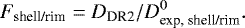
where Ṙshell/rim are the true expansion velocities of the rim orshell edges (in km s−1) and  the corresponding angular expansions in the plane of sky (in mas yr−1). The true edge (shock) expansion velocities cannot be measured and must be gained via the measured line-of-sight Doppler velocities and appropriate correction factors: F = Ṙshell/rim∕Vshell/rim > 1, so that
 (3)
(3)
One must distinguish between shell and rim because it is a priori not guaranteed that the same correction factor is valid for shell and rim. In any case, shell and rim should give the same expansion distance if the underlying physical model is correct.
The need for these correction factors is usually ignored in the literature, although their significance has already been pointed out by Marten et al. (1993). Later these corrections were quantified analytically by Mellema (2004) and by means of hydrodynamical simulations by Schönberner et al. (2005b) and SBJ. They are important because they increase the distance considerably, namely from about 30% up to about 100%, depending on the expansion state of the object considered, namely the properties of the respective shocks.
Detailed and internally consistent 1D radiation-hydrodynamics simulations of planetary-nebula formation and evolution (Schönberner et al. 1997; Perinotto et al. 1998, 2004; Villaver et al. 2002; Steffen & Schönberner 2006) suggest that indeed the physical system of a planetary nebula mainly consists of two nested shock waves that expand independently from each other. The faint (outer) shell, which also contains most of the nebular mass, is driven by thermal pressure while the optically bright inner rim is the result of wind interaction: a bubble of hot, shocked-wind gas expands against the thermal pressure of the ionised shell gas. A sketch of the main constituents of a PN is shown in Fig. 1.
In this paradigm it is important to realise that the shell’s shock is completely decoupled from the stellar wind by the rim. The stellar wind, with possible asymmetries introduced by a binary central star already earlier on the AGB, only sets the stage and influences, but does not control, the further dynamical evolution of the main part of a PN across the Hertzsprung–Russell diagram (HRD).
The different properties and evolutionary histories of shell and rim have also been found by Mellema (1994, 1995) in his somewhat parameterised hydrodynamical studies on the formation and evolution of PNe. Consequently, he coined the term “I-shock” forthe leading shock of the shell in order to indicate that it is set up by ionisation, and the term “W-shock” for the shock preceding the rim because the latter is the result of wind-wind interactions. Unfortunately, both terms could not find acceptance in the literature.
Becauseof the different expansion behaviour of rim and shell, their leading shocks are expected to have different properties and thus correction factors as well. In SBJ the correction factors were carefully evaluated from the hydrodynamical models. As expected, both the inner bright rim and the outer shell demand different correction factors, reflecting the differentdriving mechanisms of rim and shell. More details can be found in Schönberner et al. (2014) and SBJ.
In short, if Ṙshell is the propagation speed of the shell’s shock front and Vpost the corresponding post-shock flow velocity3, the relation
 (4)
(4)
holds, virtually independent of the evolutionary state as long as the nebula is optically thin. In fact, Jacob et al. (2013, Fig. 9 therein) showed that Fshell varies between about 1.2 and 1.4, depending on the parameters of the hydrodynamical sequences. The value chosen in SBJ and used here is typical for nebula models around nuclei with masses below 0.6 M⊙. If instead of the post-shock velocity only a “bulk” expansion velocity of the shell is available, the value of Fshell is accordingly higher, namely about 1.5.
The situation is different for the rim because (i) one can only measure the rim’s bulk expansion, defined by half the peak separation of the split rim line emission, and (ii) the rim’s expansion is strongly accelerating with time. We write
 (5)
(5)
where Frim is a decreasing function of the rim velocity: Frim ≃ 3 for Vrim = 5 km s−1 and Frim ≃ 1.5 for Vrim = 20 km s−1 (Fig. 5 in SBJ). These numbers refer to measurements of [O III] lines and may change if lines of other ions are used. We remark further that all studies prior to SBJ used uncorrected rim expansions only, leading to considerable underestimations of the distances by at least 50%.
We repeat here that the correction factors to be applied to Eq. (1) must always be larger than unity according to the physics of shock propagation (e.g. Mellema 2004), so that disregarding them will lead to a systematic underestimation of distances. Support for the reliability of the correction factors as introduced and discussed here comes from the fact that in the three cases where both rim and shell proper motions are available the rim and shell distances agree within the errors (Fig. 7 in SBJ).
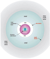 |
Fig. 1 Sketch of the main constituents of a PN mentioned in the text; it is not to scale. |
3 Expansion versus Gaia DR2 distances
We found 11 PNe in the Gaia DR2 catalogue that are in common with objects for which SBJ have derived expansion parallaxes. In general, the accuracy of the Gaia parallaxes is comparable to or even higher than for the expansion parallaxes. Except for IC 4593, the errors of the Gaia parallaxes are well below about 15%, and in two cases, NGC 3132 and NGC 6826, even below 10%. In three cases (red in Fig. 2), IC 2448, NGC 5882, and NGC 7662, the Gaia photometry of the central star is not consistent with the respective ground-based photometry. However, we verified by the Gaia software services provided by Astromisches Rechen-Institut, University of Heidelberg, that Gaia was locked onto the central star also in these cases. Furthermore, the relative errors of Gaia’s phot_g_mean_flux are very small, comparable to the other objects. NGC 7009 has the highest flux error of the whole sample, namely 0.4%. Recalling that photometry of central stars from the ground may sometimes be difficult because of a high background, we do not see any reason to exclude IC 2448, NGC 5882, and NGC 7662 from the Gaia comparison sample.
All the relevant data on expansion and trigonometric Gaia distances of our 11 sample objects are given in Table 1, supplemented by the uncorrected expansion distances as they follow separately for shell and rim (Cols. 5 and 8) together with the corresponding (Doppler) expansion velocities (Cols. 6 and 9) and correction factors (Cols. 7 and 10).
A comparison between the expansion and the Gaia distance sets is displayed in Fig. 2. Except for the two outliers IC 2448 and NGC 6891 which deserve further discussion, the data points follow closely a 1:1 relation. The linear regression considering all 11 objects and forced to go through the origin is
 (6)
(6)
where the error bars in both directions were properly taken into account in the determination of the best fitting slope and its error. Considering only the eight objects with Gaia DR2 distances below 2 kpc, we obtain
 (7)
(7)
Our sample of 11 PNe with known expansion distances and existing Gaia DR2 trigonometric distances.
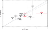 |
Fig. 2 Expansion distances, Dexp, of PNe versus the trigonometric Gaia DDR2 distances (Cols. 3 and 4 of Table 1). The dashed line is the error weighted linear regression forced to go through the origin (Eq. (6)). The dotted line represents the corresponding linear regression for the eight objects with DDR2 < 2 kpc only (Eq. (7)). The 1:1 relation is given for comparison as well (solid). For the red objects (IC 2448, NGC 5882, NGC 7662), discrepancies between the terrestrial and Gaia photometry of the central star exist (see text for details). |
3.1 Comments on individual objects
Here we compare the new Gaia DR2 distances with other individual distances, if available, notably with those based on detailed stellar spectroscopy by Méndez et al. (1992), Pauldrach et al. (2004), and Kudritzki et al. (2006), and/or with distances found from a modelling of the entire star-nebula system. Such a comparison is important because PNe with spectroscopically derived distances have frequently been used as highly weighted calibrators for statistical distance scales in the past (see e.g. Frew et al. 2016). For the sake of brevity, we considered results from the more recent literature only.
IC 418
This object is the least evolved of our sample and on the verge of becoming optically thin. The visible PN is still surrounded by a huge photo-dissociation region (cf. Gómez-Llanos et al. 2018). We face the difficulty of choosing the proper combination of flow velocity and correction factor for the shell. The two existingexpansion parallax measurements of Guzmán et al. (2009) and SBJ yielded distances of 1.30 ± 0.40 kpc and 1.15 ± 0.20 kpc, respectively, somewhat lower than the trigonometric distance found by Gaia,  kpc. The higher trigonometric distance makes the nucleus of IC 418, with 11 200 ± 2900 L⊙, the most luminous (and also most massive, ≃ 0.66 M⊙, Miller Bertolami 2016) of our sample, comparable to the most luminous object in the Milky Way bulge sample of Hultzsch et al. (2007), which has ≃ 10 200 L⊙.
The Gaia DR2 distance to IC 418 agrees perfectly with the gravity distance derived by Méndez et al. (1992), 1.5 kpc, but with a somewhat lower stellar luminosity of ≃ 9200 L⊙. The photospheric analysis of Morisset & Georgiev (2009) yielded a higher stellar gravity and consequently only a distance of 1.26 kpc and ≃ 7600 L⊙ for the central star. Upscaling to the Gaia distance yields a stellar luminosity of ≃ 11 500 L⊙. The distances of Pauldrach et al. (2004) and Kudritzki et al. (2006) are obviously too high: 2.0 and 2.6 kpc, respectively. With these distances, the central-star luminosity gets extremely high, ≃ 16 000 L⊙.
Recently, Dopita et al. (2017) presented a detailed photoionisation model of the IC 418 system and came up with a distance of 1.0 ± 0.1 pc only. This rather low value is certainly not compatible with Gaia’s trigonometric distance.
IC 2248 and NGC 6891
For these two objects, the trigonometric Gaia DR2 parallaxes are substantially lower than our expansion parallaxes, namely by a factor of about 1.7 in both cases. We do not have a reasonable explanation for this discrepancy because both objects have a rather regular elliptical shape and are thus well suited to expansion measurements. We note that our measured proper motion of NGC 2448’s rim agrees well with the older results of Palen et al. (2002), which are based on a shorter time span. The only possibility left to enlarge the expansion distance for both objects is to increase the rim correction factors Frim, namely from 1.5 to ≃2.4 (IC 2448) and from 2.3 to ≃3.7 (NGC 6891), in contradiction with the predictions from our hydrodynamical models (cf. Fig. 3 below).
NGC 6891 is a twin of NGC 6826, and for the latter expansion and trigonometric distances agree very well (see below). The rim expansion of NGC 6891, with 7 ± 1 km s−1, is the lowest of the whole sample. At such a very slow expansion of the rim, Frim is a steep function of Vrim (Fig. 3). Given the uncertainty of Vrim, Frim values of 3 or even higher are not unreasonable, which would then suffice for reaching a fair agreement with the Gaia measurement.
This procedure will not work for IC 2448 because it is a rather evolved PN with a high value of rim expansion (Vrim = 18 ± 1 km s−1) and a correspondingly moderate value of Frim = 1.5 (cf. Fig. 3). Additionally, the distance of IC 2448 from the shell expansion is even lower but still consistent within the errors with the distance based on the rim expansion (see Tables 4 and 5 in SBJ). A shell correction factor of about 2.9 (instead of 1.25) would be necessary in order to get agreement with the Gaia distance (cf. Table 1).
Méndez et al. (1992) provided distances for both objects, 3.3 kpc (NGC 2448) and 3.0 kpc (NGC 6891), which are fully consistent with the respective Gaia trigonometric distances of  kpc (IC 2448) and
  kpc (NGC 6891). Support for the higher Gaia distances comes from the fact that the expansion distance results in very low stellar luminosities for both objects, namely just a bit above 2000 L⊙ (see Table 8 in SBJ). With the Gaia trigonometric distances, more reasonable luminosities follow: 6800 ± 1500 L⊙ for IC 2448 and 6200 ± 1100 L⊙ for NGC 6891.
IC 4593
The Gaia DR2 result confirms our high expansion distance, though the error bars of the latter are the largest of the whole sample. The spectroscopic distances of Méndez et al. (1992) (3.0 kpc) and Kudritzki et al. (2006) (3.3 kpc) are still consistent within the errors, while the distance of Pauldrach et al. (2004) (3.6 kpc) is too high.
NGC 3132
This nebula has a far evolved low-luminosity nucleus, namely a hot white dwarf, and is thus optically thick (cf. SBJ). Our expansion distance is higher than the Gaia distance, but here we have again the problem of a proper combination of flow and shock expansion velocities in recombined optically thick nebulae without a double-shell structure. It appears that our chosen flow velocity or correction factor is somewhat too high. We note that an empirical rim correction factor of about unity as found by us (Col. 10 in Table 1) is not in conflict with hydrodynamical PN models in their final recombination/reionisation phase (see top panels of Fig. A.1 in SBJ). We also remark that NGC 3132 has the lowest distance of all the sample objects from Table 1 and thus also the smallest parallax error.
NGC 3242
Already SBJ gave a higher distance to NGC 3242 than found in earlier expansion works and discussed the reasons. Gómez-Muñoz et al. (2015) analysed the same HST images as were used by SBJ, but came up with a distance of 0.66 ± 0.10 kpc only. The reason is the neglect of the correction factor, which is about 1.6 in this particular case. Considering this factor, a distance of 1.06 ± 0.16 kpc follows, virtually the same as the SBJ value of 1.15 ± 0.15 kpc, as one would expect (compare Cols. 4 and 6 in Table 1). The Gaia value,  , is higher, but the errors just overlap.
For this object, the spectroscopic gravity distances are all rather close to the expansion and Gaia values: 1.7 kpc (Méndez et al. 1992; Kudritzki et al. 2006) and 1.1 kpc (Pauldrach et al. 2004). With a distance to NCG 3242 of 1.47 kpc, the luminosity of its nucleus increases from ≃3000 L⊙ (1.15 kpc, Table 8 in SBJ) to ≃ 5400 L⊙, a very reasonable value.
In this context, we note that Barría & Kimeswenger (2018) published recently a photoionisation study of the entire NGC 3242 system. Using the wrong distance of 0.66 kpc of Gómez-Muñoz et al. (2015), they found for the central star a luminosity of ≃ 5500 L⊙, which is obviously an unrealistic combination of distance and luminosity: scaling formally this luminosity value to the Gaia trigonometric distance of 1.47 kpc, a completely unreasonable central-star luminosity of about 27 000 L⊙ follows.
NGC 5882
The detailed photoionisation modelling of Miller et al. (2019) yielded a distance of  kpc and a stellar luminosity of
  L⊙. This distance is well in between the expansion (1.7 ± 0.30 kpc) and trigonometric Gaia (
 kpc) values. Using the Gaia parallax, the central-star luminosity increases somewhat, namely to ≃3400 L⊙.
NGC 6543
The shell of NGC 6543 appears to be rather complex, but the rim is more regular and allowed a reliable expansion distance to be determined, 1.86 ± 0.15 kpc (SBJ), which is only slightly higher than the Gaia trigonometric distance of  kpc. The modelling of star and nebula by Georgiev et al. (2008) yielded a distance of 1.8 kpc, but unfortunately the authors discarded this value and replaced it by Reed et al. (1999)’s expansion distance of 1 kpc and rescaled their model accordingly. Using the Gaia distance instead, a reasonable luminosity of 4200 L⊙ follows.
The expansion distance of Reed et al. (1999) is, of course, too low because the authors did not correct for the difference between pattern and matter velocities. Applying the rim correction factor used by SBJ, namely 1.5, Reed et al.’s expansion distance fully agrees with the Gaia value.
NGC 6826
This is a very interesting object because Pauldrach et al. (2004) found extreme values for central-star mass and luminosity: 1.4 M⊙ and 15 800 L⊙ in combination with a distance of 3.2 kpc. Gaia DR2 fully confirms the SBJ expansion parallax in that the distance to NGC 6826 is only half as much, namely  with a low error of only about 7%. The stellar luminosity would then be only about 3900 L⊙, more in line with the mean “plateau” luminosity of the other sample stars of ≃ 5000 L⊙ (SBJ). While Kudritzki et al. (2006) estimated also a similarly high distance of 2.5 kpc, the gravity distance derived by Méndez et al. (1992), 1.8 kpc, is rather close to the Gaia value.
There are several studies of the whole system available from the literature. The most recent one is that of Barría & Kimeswenger (2018, Table 2 therein) who found a distance of 2.1 ± 0.5 and 6000 L⊙. This distance is just compatible with the Gaia value within the uncertainties. We note, however, that their nebular modelling resulted in a stellar effective temperature of 65 000 K, much too high for the spectral appearance of the star, which suggests an effective temperature between 45 000 and 50 000 K only (see e.g. Méndez et al. 1992; Pauldrach et al. 2004; Kudritzki et al. 2006).
The earlier study of nebula plus star by Fierro et al. (2011) came to a completely different result: 0.8 ± 0.2 kpc and 6000 L⊙ with Teff = 45 000 K. Still other parameters were found by Surendiranath & Pottasch (2008). From a Cloudy photoionisation model, the authors derived a best-fit stellar model with distance 1.40 kpc, 1640 L⊙, and with Teff = 47 500 K. Surendiranath & Pottasch 2008 presented arguments “which strongly rule out a higher luminosity than given by us”.
It appears to us difficult to reconcile the results of these three studies. Scaling the different luminosities found for the central star of NGC 6826 to the Gaia distance, we end up with 3400 L⊙ (Barría & Kimeswenger 2018), 23 400 L⊙ (Fierro et al. 2011), and 2090 L⊙ (Surendiranath & Pottasch 2008). On the other hand, the downscaling of the gravity distances to the Gaia distance leads to more realistic but still diverse luminosities for the central star of NGC 6826: 7200 L⊙ (Méndez et al. 1992), 3900 L⊙ (Pauldrach et al. 2004), and 4800 L⊙ (Kudritzki et al. 2006).
NGC 7009
Although this object has an irregular rim, the expansion distance derived from the proper motion of the semi-minor axis agrees within the errors with the Gaia DR2 value (see Table 1)4. With the new Gaia distance, the central-star luminosity is lower than found by SBJ, namely from 4750 to 2800 L⊙. The gravity distance of Méndez et al. (1992) is nearly twice as high as the Gaia distance: 2.1 kpc.
NGC 7662
Here again both the expansion and the trigonometric Gaia distances agree very well (Table 1), but they do not agree with the much lower distance of 1.19 ± 0.15 kpc given by Barría & Kimeswenger (2018) by means of photoionisation modelling. As in the case of NGC 3242, this combination of distance with the stellar luminosity ≃ 5300 L⊙ appears to be strange because increasing the distance to the Gaia value would result in an excessively high luminosity of about 15 700 L⊙. In contrast, the modelling of Miller et al. (2019) provided a distance consistent with both the expansion and Gaia distances:  , together with a central-star luminosity of
  L⊙.
L⊙.
4 Empirical determination of the hydrodynamical correction factors F
Figure 2 and the discussion of the sample objects have already demonstrated that distances derived by just combining line-of-sight Doppler velocities with proper motions of suited shock fronts must be corrected by appropriately chosen factors, which are usually well above unity. Tables 4 and 5 in SBJ contain separately the information on shell and rim expansions, the used corrections, and the distances that follow thereby. For convenience, we give in Cols. 5 and 6 of Table 1 also the uncorrected distances that follow directly from the SBJ expansion measurements by using Eq. (1). With known trigonometric distances from Gaia, this opens up the possibility to determine empirically the correction factors for both the shell and rim separately, including also their dependence on evolution.
The case is illustrated in Fig. 3 where we show (NGC 3132 excepted), separately for shell and rim, the empirically determined correction factors from Table 1 (Cols. 7 and 10). They are defined by the ratio between the Gaia trigonometric distance and the respective expansion distance without considering any correction:
 (8)
(8)
We plotted the F factors against their respective Doppler velocities, Vpost or Vrim, because the latter are a measure of the hydrodynamical state of a PN. They are also a measure of the evolutionary progress since it was shown empirically in Schönberner et al. (2014) that both velocities increase during evolution across the HRD, albeit at different paces.
First of all, Fig. 3 confirms that the correction factors are always greater than one for both the shell and rim expansion. Their sizes and their run with evolution are, however, quite different.
Shell
Fshell appears indeed to be independent of the shell’s expansion, which in turn also implies that the property of the shell’s shockdoes not really change while the central star crosses the HRD: the temperatures of the four objects in the top panel of Fig. 3 span the range from about 40 000 K (IC 418 and IC 9543) to ≃120 000 K (NGC 7662). With the exception of the “outlier” IC 2448, the individual shell correction factors of the sample objects are, within the errors, fully consistent with the prediction of our hydrodynamical models (thick dashed line at Fshell = 1.25).
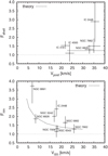 |
Fig. 3 Correction factors Fshell and Frim, defined according to Eq. (8), as function of the respective (line-of-sight) Doppler expansions: the shell’s post-shock velocity Vpost (top panel) and the rim’s bulk expansion velocity Vrim (bottom panel). The crosses indicate the empirically determined F values for individual objects, where their error bars are derived from the sums of the relative error squares of the trigonometric and expansion distances. The thick dotted lines are the theoretical expectations from hydrodynamical models, namely a constant value of 1.25 for the shell and an average from the model curves in Fig. 5 of SBJ for the rim. The weakly dotted horizontal lines highlight unity. Evolution is always from low to high velocities (see text for details). The correction factor of NGC 3132 is not plotted here because this particular nebula is the most evolved of the whole sample and is in its recombination or reionisation phase, which is not covered by the hydrodynamical models employed for the determination of the correction factors. |
Rim
The situation is different for the rim (bottom panel). Here, the correction factor Frim is predicted to decrease with increasing rim expansion. This trend is obviously confirmed by the Gaia measurements. The stellar temperaturerange is similar to that of the shell: from about 50 000 K (NGC 6826) to about 120 000 K (NGC 7662). NGC 6891 has the lowest rim expansion and the biggest empirical rim correction of all sample objects, although the uncertainty is very high.
We especially comment on the two objects that are contained in both panels of Fig. 3: NGC 6826 and NGC 7662. The former object is rather young with a still slowly expanding rim, while NGC 7662 is far more evolved with its hot central star.Hence, the correction factors differ considerably (cf. Cols. 7 and 10 in Table 1): Fshell ≃ 1.3 ± 0.2 and Frim ≃ 1.9 ± 0.3 for NGC 6826, in very closeagreement with the prediction of our hydrodynamical models. For the evolved object NGC 7662, both corrections are very similar: Fshell ≃ 1.5 ± 0.4 and Frim ≃ 1.3 ± 0.3, also consistent with the models.
5 Summary and conclusion
We compared the trigonometric parallaxes of 11 PNe contained in the recent Gaia DR2 with the corresponding expansion parallaxes that were based on multi-epoch HST images in combination with Doppler expansion velocities and appropriate corrections derived from 1D hydrodynamical models. From these 11 objects, only two objects, IC 2448 and NGC 6891, have discrepant distances for reasons we can only speculate about. For the rest, a quite narrow 1:1 relation for the whole distance range from about 1 to 3 kpc exists. This agreement could only be achieved by means of correction factors that take account of the hydrodynamics and of the fact that the expansion method combines pattern expansion (i.e. that of shock fronts) with matter velocities (gas flow velocities).
Our main conclusion is that the Gaia data not only confirm the necessity of corrections for the expansion parallaxes just as they have been derived in SBJ, but also that they are different for rim and shell. This also proves that the evolution of round or elliptical planetary nebulae is correctly described already by the 1D hydrodynamical models of Villaver et al. (2002) and Perinotto et al. (1998, 2004). In particular, we also can conclude the following:
-
the well-known interacting winds paradigm for the formation and evolution of PNe cannot be applied to the shell, that is, to most of the nebula mass. The shell’s formation is caused by photoionisation, and its following expansion is ruled by thermal pressure and the upstream density gradient. The shell’s shock does not “know” the existence of a stellarwind. The latter only fills up nearly the entire cavity left by the expanding shell with shock-heated and thermalised wind matter (the hot bubble).
-
In contrast, the rim is the product of wind interactions and is formed once the shell is established: the increasing thermal pressure of the hot bubble forces the latter to expand and to compress the inner parts of the shell, and the rim’s further expansion is ruled by the bubble’s pressure, which in turn depends on the evolution of the stellar wind luminosity.
-
The Gaia DR2 results also confirm the findings of SBJ that the spectroscopically derived distances have the tendency to be overestimated. This fact needs further investigations and may also lead to an improvement of the stellar atmosphere and/or wind modelling.
-
Really disturbing is the fact that elaborate analyses of the combined system, nebula and central star, may not always lead to parameters consistent with the values inferred from the Gaia distances.
Finally, we note that the (geometrically) thin rim is subject to dynamical instabilities, but these are obviously not as strong as the 2D simulations of spherical model nebulae performed by Toalá & Arthur (2016) suggest. Otherwise, rims as observed would not exist, and the determination of reasonable expansion parallaxes from the rims would not have been possible. It is hoped that future 3D simulations with sufficient spatial resolution will improve this issue.
Acknowledgements
We are very grateful to Dr. Stefan Jordan, Astronomisches Rechen-Institut am Zentrum für Astronomie der Universität Heidelberg, for his help in interpreting the relevant Gaia DR2 data. We thank the referee for his or her very useful comments that helped us to improve the presentation of the paper.
References
- Barría, D., & Kimeswenger, S. 2018, MNRAS, 480, 1626 [NASA ADS] [CrossRef] [Google Scholar]
- Benedict, G. F., McArthur, B. E., Napiwotzki, R., et al. 2009, AJ, 138, 1969 [NASA ADS] [CrossRef] [Google Scholar]
- Corradi, R. L. M., Steffen, M., Schönberner, D., & Jacob, R. 2007, A&A, 474, 529 [NASA ADS] [CrossRef] [EDP Sciences] [Google Scholar]
- Dopita, M. A., Ali, A., Sutherland, R. S., Nicholls, D. C., & Amer, M. A. 2017, MNRAS, 470, 839 [NASA ADS] [CrossRef] [Google Scholar]
- Fierro, C. R., Peimbert, A., Georgiev, L., Morisset, C., & Arrieta, A. 2011, Rev. Mex. Astron. Astrofis., Ser. de Conf., 40, 167 [NASA ADS] [Google Scholar]
- Frew, D. J., Parker, Q. A., & Bojičić, I. S. 2016, MNRAS, 455, 1459 [NASA ADS] [CrossRef] [Google Scholar]
- Gaia Collaboration (Brown, A. G. A., et al.) 2016a, A&A, 595, A2 [NASA ADS] [CrossRef] [EDP Sciences] [Google Scholar]
- Gaia Collaboration (Prusti, T., et al.) 2016b, A&A, 595, A1 [NASA ADS] [CrossRef] [EDP Sciences] [Google Scholar]
- Gaia Collaboration (Brown, A. G. A., et al.) 2018, A&A, 616, A1 [NASA ADS] [CrossRef] [EDP Sciences] [Google Scholar]
- Georgiev, L. N., Peimbert, M., Hillier, D. J., et al. 2008, ApJ, 681, 333 [NASA ADS] [CrossRef] [Google Scholar]
- Gómez-Llanos, V., Morisset, C., Szczerba, et al. 2018, A&A, 617, A85 [NASA ADS] [CrossRef] [EDP Sciences] [Google Scholar]
- Gómez-Muñoz, M. A., Blanco Cárdenas, M. W., Vázquez, R., et al., 2015, MNRAS, 453, 4175 [NASA ADS] [Google Scholar]
- Guzmán, L., Loinard, L., Gómez, Y., & Morisset, C. 2009, AJ, 138, 46 [NASA ADS] [CrossRef] [Google Scholar]
- Harris, H. C., Dahn, C. C., Canzian, B., et al. 2007, AJ, 133, 631 [NASA ADS] [CrossRef] [Google Scholar]
- Hultzsch, P. J.N., Puls, J., Méndez, R. H., et al. 2007, A&A, 467, 1253 [NASA ADS] [CrossRef] [EDP Sciences] [Google Scholar]
- Jacob, R., Schönberner, D., & Steffen, M. 2013, A&A, 558, A78 [NASA ADS] [CrossRef] [EDP Sciences] [Google Scholar]
- Kimeswenger, S., & Barría, D., 2018, A&A, 616, L2 [NASA ADS] [CrossRef] [EDP Sciences] [Google Scholar]
- Kudritzki, R.P., Urbaneja, M.A., & Puls, J. 2006 in Planetary Nebulae in our Galaxy and Beyond, eds. M. J. Barlow, & R. H. Méndez, IAU Symp., 234,119 [NASA ADS] [CrossRef] [Google Scholar]
- Marten, H., Gȩsicki, K., & Szczerba, R. 1993, in Planetary Nebulae, eds. R. Weinberger, & A. Acker, IAU Symp., 155, 315 [NASA ADS] [Google Scholar]
- Mellema, G. 1994, A&A, 290, 915 [NASA ADS] [Google Scholar]
- Mellema, G. 1995, MNRAS, 277, 173 [NASA ADS] [Google Scholar]
- Mellema, G. 2004, A&A, 416, 623 [NASA ADS] [CrossRef] [EDP Sciences] [Google Scholar]
- Méndez, R. H., Kudritzki, R. P., & Herrero, A. 1992, A&A, 260, 329 [NASA ADS] [Google Scholar]
- Miller Bertolami, M. M. 2016, A&A, 588, A25 [NASA ADS] [CrossRef] [EDP Sciences] [Google Scholar]
- Miller, T. R., Henry, R. B. C., Balick, B., et al. 2019, MNRAS, 482, 278 [NASA ADS] [Google Scholar]
- Morisset, C., & Georgiev, L. 2009, A&A, 507, 1517 [NASA ADS] [CrossRef] [EDP Sciences] [Google Scholar]
- Palen, S., Balick, B., Hajian, A. R., et al. 2002, AJ, 123, 2666 [NASA ADS] [CrossRef] [Google Scholar]
- Pauldrach, A. W. A., Hoffmann, T. L., & Méndez, R. H. 2004, A&A, 419, 1111 [NASA ADS] [CrossRef] [EDP Sciences] [Google Scholar]
- Perinotto, M., Kifonidis, K., Schönberner, D., & Marten, H. 1998, A&A, 332, 1044 [NASA ADS] [Google Scholar]
- Perinotto, M., Schönberner, D., Steffen, M., & Calonaci, C. 2004, A&A, 414, 993 [NASA ADS] [CrossRef] [EDP Sciences] [Google Scholar]
- Reed, D. S., Balick, B., Hajian, A. R., et al. 1999, AJ, 118, 243 [NASA ADS] [CrossRef] [Google Scholar]
- Schönberner, D. 1979, A&A, 79, 108 [NASA ADS] [Google Scholar]
- Schönberner, D. 1981, A&A, 103, 119 [NASA ADS] [Google Scholar]
- Schönberner, D. 1983, ApJ, 272, 708 [NASA ADS] [CrossRef] [Google Scholar]
- Schönberner, D. 2016, J. Phys. Conf. Ser. 728, 032001 [CrossRef] [Google Scholar]
- Schönberner,D., Steffen, M., Stahlberg, J., Kifonidis, K., & Blöcker, T. 1997, Workshop Stellar Ecology: Advances in Stellar Evolution (Cambridge: Cambridge University Press), 146 [Google Scholar]
- Schönberner, D., Jacob, R., Steffen, M., et al. 2005a, A&A, 431, 963 [NASA ADS] [CrossRef] [EDP Sciences] [Google Scholar]
- Schönberner, D., Jacob, R., & Steffen, M. 2005b, A&A, 441, 573 [NASA ADS] [CrossRef] [EDP Sciences] [Google Scholar]
- Schönberner, D., Jacob, R., Lehmann, H., et al. 2014, Astron. Nachr., 335, 378 [NASA ADS] [CrossRef] [Google Scholar]
- Schönberner, D., Balick, B., & Jacob, R. 2018, A&A, 609, A126 [NASA ADS] [CrossRef] [EDP Sciences] [Google Scholar]
- Stanghellini, L., & Haywood, M. 2010, ApJ, 714, 1096 [NASA ADS] [CrossRef] [Google Scholar]
- Stanghellini, L., Bucciarelli, B., Lattanzi, M. G., & Morbidelli, R. 2017, New Astron., 75, 5 [Google Scholar]
- Steffen, M., & Schönberner, D. 2006, in Planetary Nebulae in our Galaxy and Beyond, eds. M. J. Barlow, & R. H. Méndez, IAU Symp., 234, 285 [NASA ADS] [CrossRef] [Google Scholar]
- Surendiranath, R., & Pottasch, S. R. 2008, A&A, 483, 519 [NASA ADS] [CrossRef] [EDP Sciences] [Google Scholar]
- Toalá, J. A., & Arthur, S. J. 2016, MNRAS, 463, 4438 [NASA ADS] [CrossRef] [Google Scholar]
- Villaver, E., Manchado, A., & García-Segura, G. 2002, ApJ, 581, 1204 [NASA ADS] [CrossRef] [Google Scholar]
For more details, the reader is referred to Sect. 5.2 in Schönberner et al. (2018).
See www.nublado.org
The determination of the flow velocity immediately behind the leading shock of the shell by means of high-resolution spectrograms is discussed in detail in Corradi et al. (2007).
The distance of NGC 7009 listed in Table 8 of SBJ is incorrect. It should read 1.5 ± 0.35 kpc as in Table 7 therein and in our Table 1. The stellar parameters are not affected by this typo.
All Tables
Our sample of 11 PNe with known expansion distances and existing Gaia DR2 trigonometric distances.
All Figures
|
Fig. 1 Sketch of the main constituents of a PN mentioned in the text; it is not to scale. |
| In the text | |
|
Fig. 2 Expansion distances, Dexp, of PNe versus the trigonometric Gaia DDR2 distances (Cols. 3 and 4 of Table 1). The dashed line is the error weighted linear regression forced to go through the origin (Eq. (6)). The dotted line represents the corresponding linear regression for the eight objects with DDR2 < 2 kpc only (Eq. (7)). The 1:1 relation is given for comparison as well (solid). For the red objects (IC 2448, NGC 5882, NGC 7662), discrepancies between the terrestrial and Gaia photometry of the central star exist (see text for details). |
| In the text | |
|
Fig. 3 Correction factors Fshell and Frim, defined according to Eq. (8), as function of the respective (line-of-sight) Doppler expansions: the shell’s post-shock velocity Vpost (top panel) and the rim’s bulk expansion velocity Vrim (bottom panel). The crosses indicate the empirically determined F values for individual objects, where their error bars are derived from the sums of the relative error squares of the trigonometric and expansion distances. The thick dotted lines are the theoretical expectations from hydrodynamical models, namely a constant value of 1.25 for the shell and an average from the model curves in Fig. 5 of SBJ for the rim. The weakly dotted horizontal lines highlight unity. Evolution is always from low to high velocities (see text for details). The correction factor of NGC 3132 is not plotted here because this particular nebula is the most evolved of the whole sample and is in its recombination or reionisation phase, which is not covered by the hydrodynamical models employed for the determination of the correction factors. |
| In the text | |
Current usage metrics show cumulative count of Article Views (full-text article views including HTML views, PDF and ePub downloads, according to the available data) and Abstracts Views on Vision4Press platform.
Data correspond to usage on the plateform after 2015. The current usage metrics is available 48-96 hours after online publication and is updated daily on week days.
Initial download of the metrics may take a while.