| Issue |
A&A
Volume 624, April 2019
|
|
|---|---|---|
| Article Number | L7 | |
| Number of page(s) | 10 | |
| Section | Letters to the Editor | |
| DOI | https://doi.org/10.1051/0004-6361/201935459 | |
| Published online | 10 April 2019 | |
Letter to the Editor
Stringent limits on the magnetic field strength in the disc of TW Hya
ALMA observations of CN polarisation
1
Department of Space, Earth and Environment, Chalmers University of Technology, Onsala Space Observatory, 439 92 Onsala, Sweden
e-mail: wouter.vlemmings@chalmers.se
2
Max-Planck-Insitut für Extraterrestrische Physik, Gießenbachstrasse 1, 85748, Garching, Germany
3
Leiden Observatory, Leiden University, PO Box 9513, 2300 RA Leiden, The Netherlands
4
European Southern Observatory, Karl-Schwarzschild-Str. 2, 85748 Garching bei München, Germany
5
INAF – Osservatorio Astrofisico di Arcetri, Largo E. Fermi 5, 50125 Firenze, Italy
6
Excellence Cluster Universe, Boltzmannstr. 2, 85748 Garching bei München, Germany
7
Institute for Astronomy, University of Hawaii, Honolulu, HI 96822, USA
Received:
13
March
2019
Accepted:
26
March
2019
Despite their importance in the star formation process, measurements of magnetic field strength in proto-planetary discs remain rare. While linear polarisation of dust and molecular lines can give insight into the magnetic field structure, only observations of the circular polarisation produced by Zeeman splitting provide a direct measurement of magnetic field strenghts. One of the most promising probes of magnetic field strengths is the paramagnetic radical CN. Here we present the first Atacama Large Millimeter/submillimeter Array (ALMA) observations of the Zeeman splitting of CN in the disc of TW Hya. The observations indicate an excellent polarisation performance of ALMA, but fail to detect significant polarisation. An analysis of eight individual CN hyperfine components as well as a stacking analysis of the strongest (non-blended) hyperfine components yields the most stringent limits obtained so far on the magnetic field strength in a proto-planetary disc. We find that the vertical component of the magnetic field |Bz| < 0.8 mG (1σ limit). We also provide a 1σ toroidal field strength limit of <30 mG. These limits rule out some of the earlier accretion disc models, but remain consistent with the most recent detailed models with efficient advection. We detect marginal linear polarisation from the dust continuum, but the almost purely toroidal geometry of the polarisation vectors implies that his is due to radiatively aligned grains.
Key words: magnetic fields / accretion, accretion disks / stars: pre-main sequence / stars: individual: TW Hya
© ESO 2019
1. Introduction
There have been significant efforts to observationally determine the role of magnetic fields across all scales of star formation. For example, through magnetic viscosity, the field plays a crucial role in disc evolution and planet formation (e.g., Lizano et al. 2016), and the poloidal component of the magnetic field is responsible for disc winds (Blandford & Payne 1982). The poloidal component of the disc magnetic field is the result of magnetic flux that is dragged into the disc during proto-stellar collapse, and its strength is expected to be greater than the molecular cloud magnetic field (e.g., Ferreira & Pelletier 1995; Jafari & Vishniac 2018). However, recent models show that the toroidal magnetic field is likely the dominant component. Different models therefore cover a wide range of possible values for the poloidal field, ranging from (sub-)mG (e.g., Okuzumi et al. 2014) to tens of mG (Shu et al. 2007).
Measurements of magnetic field strengths have relied on indirect estimates from dust polarisation and on the use of the Chandrasekhar-Fermi method (e.g., Houde et al. 2009) or direct measurements of the Zeeman effect of OH, HI, or masers (e.g., Vlemmings et al. 2010, 2017; Crutcher 2012). Additionally, the Goldreich-Kylafis effect (Goldreich & Kylafis 1981, 1982), observed mainly for CO, has been used to determine magnetic field morphology (e.g., Cortes et al. 2005). However, the success of magnetic field observations of accretion or proto-planetary discs has been very limited (e.g., Hughes et al. 2009, 2013). Furthermore, it has been shown that self-scattering and radiative grain alignment further complicate the interpretation of dust polarisation (e.g., Kataoka et al. 2015, 2017). With the exception of a ∼1 kG magnetic field detection at the innermost edge (at ∼0.05 au) of the disc around FU Orionis (Donati et al. 2005), there are no direct measurements of the magnetic field strength in an accretion disc.
One of the best probes of disc magnetic fields is the CN radical, which is very sensitive to the Zeeman effect. Here we present the first ALMA CN circular polarisation observations of the CN emission arising in the disc of the T Tauri star TW Hya.
TW Hya. TW Hya, at d = 60 pc (Gaia Collaboration 2018), is a star of type K7 with an age of ∼8−10 Myr. It still actively accretes, with an accretion rate of ∼10−9 M⊙ yr−1 (Debes et al. 2013). The star has a surface magnetic field strength of ∼3 kG (Donati et al. 2011; Sokal et al. 2018). Its proto-planetary disc is massive, Mgas ∼ 0.01 M⊙, and large, extending to ∼230 au in the gas lines. The TW Hya disc has an almost face-on geometry, with i ∼ 5° (Huang et al. 2018), and the molecular lines therefore suffer only very little line-broadening due to Keplerian motion, which results in line widths of ∼0.3 km s−1 (Teague et al. 2016). The structure of the disc is well described (e.g., Bergin et al. 2013; Andrews et al. 2016; Kama et al. 2016; Teague et al. 2018). Its CN emission shows a well-resolved ring-like structure because its chemistry is driven by UV radiation (Cazzoletti et al. 2018).
CN Zeeman splitting. The CN radical was one of the first molecules that was deteced in space. Because CN is a paramagnetic molecule, it exhibits a strong Zeeman effect under the influence of a magnetic field. It also has a large number of hyperfine components. We present a calculation of the exact Zeeman splitting for the CN hyperfine components in the ALMA band 3, 6, and 7 frequency range in Appendix A. So far, CN has been used to measure the magnetic field in a handful of molecular clouds (e.g., Crutcher et al. 1996, 1999; Falgarone et al. 2008; Hezareh & Houde 2010) and around a small number of evolved stars (Duthu et al. 2017).
2. Observations and data reduction
These observations of TW Hya were performed as part of ALMA project 2018.1.00167.S on 2018 December 11, 12, and 13. The total observing time in full polarisation mode was 8.8 h, of which ∼3.6 h were spent on TW Hya. In order to reach the lowest possible spectral resolution for the Zeeman splitting experiment, we tuned three spectral windows (spws) with a width of 58.59 MHz and 1920 channels to cover 11 CN (N = 2−1) hyperfine components (see Table. B.1 for a list of observed hyperfine components). After Hanning smoothing, this resulted in a velocity resolution of 0.093 km s−1. A fourth spw of 1.875 GHz with 1920 channels and ∼3 km s−1 velocity resolution was set to encompass the three narrow windows for optimal calibration transfer. The initial calibration was performed using the standard ALMA polarisation calibration scripts in CASA 5.4.0. Bandpass, flux, and gain calibration were done using the quasars J1107−4449 (bandpass, flux) and J1037−2934 (gain). J1256−0547 was used for polarisation calibration. It was noted that over the course of the observations, the gain and polarisation calibrator showed a steady and similar decrease in flux compared to the flux calibrator, which was assumed to have a constant flux of 0.72 Jy at 226.64 GHz with a spectral index of −0.8. It is therefore likely that the flux calibrator was brightening, which is also found in the ALMA calibrator catalogue. To compensate for this change and to improve the phase calibration at short time-intervals, we performed two rounds of phase and one round of amplitude self-calibration using the continuum dust emission of TW Hya in the 1.875 GHz spectral window in which emission lines were flagged. This improved the continuum total intensity (I) signal-to-noise ratio (S/N) from ∼400 to ∼2000. The self-calibration solutions were applied to all spws. Subsequently, the continuum was subtracted using the broad spw, which was extrapolated to the narrow spws. Finally, image cubes were created for all spws at the native spectral resolution in all four Stokes parameters I, Q, U, and V using Briggs weighting and a robust parameter of 0.5. The resulting beam size was 0.44 × 0.52″. We reach a channel rms in the narrow spws of σ = 1.3 mJy beam−1 for all four Stokes parameters I, Q, U, and V. In the continuum we reach σ(I, Q, U, V) = (46, 22, 22, 23) μJy beam−1. The increased noise in total intensity I is due to dynamic range limits.
3. Results
3.1. CN polarisation
We analysed the circular polarisation of the CN N = 2−1 lines in a number of different ways to extract information about the magnetic field. Because the inclination of the disc around TW Hya is low, we are mostly sensitive to the vertical component of the magnetic field |Bz|. A radial or toroidal magnetic field component will only contribute ∼10% at most to |B| along the minor and major axis of the projected disc, respectively. We first analysed the strongest CN emission peak at (−0.09″, −0.78″) offset from the continuum peak, and processed the polarisation for all the different hyperfine components separately. The position of this peak is indicated in the integrated intensity map of the strongest unblended hyperfine component (N = 2−1, J = 3/2−1/2, F = 5/2−3/2) shown in Fig. 1 (left). We did not detect any significantly circular polarisation. The limiting circular polarisation fractions with respect to the peak total intensity emission I0 and the corresponding magnetic field limits are presented in Table B.1. The individual spectra are shown in Fig. B.1.
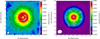 |
Fig. 1. Left panel: integrated intensity map of the CN (N = 2−1, J = 3/2−1/2, F = 5/2−3/2) hyperfine transition around TW Hya. We also indicate the line of nodes of the disc at a position angle of 240° and the location of the strongest CN emission peak that was used in the polarisation analysis (see text). Right panel: continuum and polarised 226 GHz emission of the TW Hya disc. The colour scale is the total intensity dust emission. The contours, drawn at 3 and 4σ, are the linear polarisation, and the white-line segments indicate the electric vector polarisation angle. |
Subsequently, we stacked all but the two weakest hyperfine components, correcting for their relative intensity and sensitivity to the magnetic field. Specifically, the stacked Stokes V spectrum was produced by scaling Stokes V spectra of the individual components by the relative Stokes I peak intensity and the relative magnitude of the Zeeman coefficient with respect to that of the strongest hyperfine component in the stacking analysis (CN N = 2−1, J = 5/2−3/2, F = 7/2−5/2). The resulting Stokes I and V spectra are shown in the left panel of Fig. 2. In this analysis no circular polarisation is detected either, and we reach a fractional limit (1σ) of |Bz| < 2.7 mG. Finally, we produced an azimuthally averaged spectrum that was corrected on a pixel-by-pixel basis for the Keplerian rotation of the disc. This correction is essential to reduce the line width and optimise the detectability of the circular polarisation. Because of the limited angular resolution, some line broadening remains in excess of the turbulent line width derived by Teague et al. (2016). The spectrum is taken within a ring, with a width of the synthesised beam, that includes the brightest CN emission. The ring has a radius of 0.72″, which corresponds to ∼42 au. The stacked spectrum is best represented using a line width of 0.45 km s−1. We limit this analysis to the two strongest unblended hyperfine components that are most sensitive to the magnetic field (CN N = 2−1, J = 5/2−3/2, F = 3/2−1/2 and N = 2−1, J = 3/2−1/2, F = 5/2−3/2). A stacked spectrum of the two lines is shown in the middle panel of Fig. 2. This analysis provides the tightest constraint on the magnetic field strength, and reaches a 1σ limit of |Bz| < 0.8 mG.
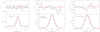 |
Fig. 2. Total intensity (I, bottom panel) and circular polarisation (V, top panel) CN spectra. The 1σ and 3σ limits are indicated by the short and long dashed lines, respectively. Left panel: spectra stacking the nine strongest CN N = 2−1 hyperfine components that we extracted at the position of the strongest emission peak. The 1σ limit corresponds to a magnetic field strength |Bz| = 2.7 mG, for which the V-spectrum is indicated in red. The effective line width is 0.45 km s−1. The apparent non-zero baseline in the Stokes I spectrum is due to the contribution to the stacked spectrum of hyperfine components that occur within 1.5 km s−1 of each other. Middle panel: azimuthally averaged spectra obtained by stacking the two strongest CN hyperfine components in our data that are not significantly blended. The rms limit corresponds to a magnetic field strength |Bz| = 0.8 mG, for which the V-spectrum is indicated in red. The effective line width is 0.45 km s−1. Beyond +0.5 km s−1, the spectrum is affected by a blend with a neighbouring hyperfine component. Right panel: similar to the middle panel, but only for emission along the line of nodes (see text). Here the signature of a toroidal field would be strongest. The fractional rms reached on the V-spectrum is 0.33%. The rms limit corresponds to a magnetic field strength |B| = 2.6 mG, for which the V-spectrum is indicated in red. This corresponds to a toroidal field strength limit of |Bϕ| < 30 mG. The effective line width is 0.5 km s−1. |
In order to provide a rough estimate on the toroidal field strength, we repeated the analysis and restricted ourselves to the CN emission in the eastern and western part of the major axis of the projected inclined disc. This corresponds to the line of nodes. In our analysis, we corrected for the expected sign difference between the two sides. As shown in the right panel of Fig. 2, we reach an rms of ∼0.33%, which requires a slightly broader line width of 0.5 km s−1. This corresponds to |Bz| < 2.6 mG or a toroidal field strength of |Bϕ|=|Bz|/sin i < 30 mG. The stacked line of nodes of the V-spectrum does display a 2σ signal that could correspond to a magnetic field strength of ∼5 mG, although it is slightly shifted (by ∼0.1 km s−1) from the expected location. If this is real, it should originate from the toroidal magnetic field because no signature is seen in the more sensitive analysis of the azimuthally averaged spectrum. The expected reversal of a toroidal field is hinted at in the eastern and western parts of the line of nodes separately, as shown in Fig. C.1, and the field strength would correspond to |Bϕ|≈57 mG. However, considering the low significance of the circular polarisation signal (∼2σ), we do not classify it as a detection.
3.2. Continuum polarisation
Although the observation setup was optimised for a line polarisation study, we were able to produce a linear polarisation image of the dust continuum emission at 226 GHz using the line-free channels of the 1.875 GHz wide spw. We debiased the linear polarisation map by calculating the linearly polarised intensity from the Stokes Q and U images using  . Here σP is the polarised rms, which can be calculated on a pixel-by-pixel basis using
  Here we adopt the σQ, U as measured in the images. We find σP ≈ 22 μJy beam−1. The resulting polarisation map is shown in Fig. 1 (right). The polarisation peaks at slightly above 4σ and ranges from <0.1% of Stokes I towards the inner part of the disc to ∼2% in the outer parts. The patchy appearance of the polarisation is likely due to the low S/N of the observations. The polarisation vectors are almost purely toroidal, which is the signature of radiatively aligned grains dominating the polarised emission (e.g., Kataoka et al. 2017). However, because of the low S/N of the polarisation and the lack of data at other wavelengths1, a discussion of the nature of the continuum polarisation is beyond the scope of this paper.
4. Discussion and conclusions
We have obtained a tight upper limit to the vertical magnetic field component using the CN emission in the disc around TW Hya. Our azimuthal average field limit of |Bz| < 0.8 mG was obtained at a radius of approximately 42 au. According to the model of CN emission from Cazzoletti et al. (2018), at this radius, we are most sensitive to the magnetic field at a disc scale height of |z|∼18 au. In terms of plasma β, the ratio of gas to magnetic pressure, this means for the vertical field component that β ≳ 4 × 10³ when we adopt the disc model used in Bai (2015).
The vertical magnetic field in a proto-planetary accretion disc is generally assumed to be advected inwards from the surrounding cloud. However, it was noted that under the influence of turbulence, a large-scale field would diffuse away at timescales much shorter than the advection timescales (see e.g., Okuzumi et al. 2014; Guilet & Ogilvie 2014, and references therein for a more detailed discussion). The details of advection and diffusion therefore strongly affect the vertical magnetic field strength. In Fig. 3 we compare our derived upper limits with predictions from the T Tauri star model of Shu et al. (2007) and the maximum vertical field strength according to the thin accretion disc model from Okuzumi et al. (2014). It is immediately apparent that our limit lies significantly below the value predicted in Shu et al. (2007). Both models depend critically on the assumed field strength outside the disc, B∞. In particular, Okuzumi et al. (2014) stated that Bz, max = (Rout/R)2B∞. Because we measure our limit at R ∼ 42 au and Rout ∼ 230 au for the disc of TW Hya, our limit would thus imply B∞ < 25 μG. While such fields are consistent with Zeeman measurements in diffuse molecular clouds (e.g., Crutcher 2012), the fields measured in proto-stellar envelopes and dense cloud regions are much higher and of order 1−10 mG (e.g., Girart et al. 2006; Houde et al. 2009; Vlemmings et al. 2010).
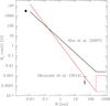 |
Fig. 3. Vertical magnetic field strength (Bz) from accretion disc models, compared with the 1σ limit obtained in our ALMA observations (Bz < 0.8 mG, indicated by the arrow). The solid line is the T Tauri model from Shu et al. (2007). The dotted line is the maximum field strength Bz, max from Okuzumi et al. (2014), taking a magnetic field strength at the outer edge of the disc (Rout = 230 au) of B∞ = 25 μG. The red long dashed line assumes B∞ = 1 mG, which corresponds to the field strength measured in proto-stellar cores and dense parts of molecular clouds, and it includes efficient advection with D = 0.025 (see text). At R < 230 au, the latter two models are identical. The solid circle shows the surface magnetic field measured on TW Hya (e.g., Sokal et al. 2018). |
Depending on the details of advection and diffusion, the vertical field strength should be described as Bz = D(R)⋅(Rout/R)2B∞, where D(R) is defined as the inverse ratio of advection to diffusion timescales (e.g., Okuzumi et al. 2014). In the case of effective advection that overcomes the diffusion of the magnetic field, D(R) << 1 in the disc (where R < Rout). In the case of TW Hya, we thus find that D(42 au) < 0.025/B∞ for B∞ given in mG. Even though this limit on D depends on the unknown magnetic field strength in the original proto-stellar envelope around TW Hya, our observations present the first observational constraint of the advection in an accretion disc.
A number of studies have also related the vertical magnetic field strength to the disc accretion rate (e.g., Okuzumi & Hirose 2011; Bai 2013; Simon et al. 2013). Using the relation obtained for magneto-rotational instability-driven accretion in the case of only Ohmic diffusion (Okuzumi & Hirose 2011; Okuzumi et al. 2014), our limit implies Ṁ ≲ 3 × 10⁻⁷ M⊙ yr−1. A limit of Ṁ ≲ 8 × 10⁻⁸ M⊙ yr−1 is obtained when models are used in which ambipolar diffusion is taken into account (Bai 2013; Simon et al. 2013). These limits are fully consistent with the accretion rates derived for the evolved TW Hya disc.
These limits are determined using models that assume a fixed configuration of the magnetic field without a toroidal component and/or without treating thermodynamics. Relaxing these assumptions can lead to a dominant toroidal field component with a strength of ∼10−15 mG (Bai 2015), which is consistent with the toroidal field limits we derived.
Despite the non-detection, our observations show that ALMA is able to reach detection levels in circular polarisation of <0.8% of the total intensity. The stacking analysis further shows no sign of instrumental effects at even lower levels. This shows that for relatively strong and narrow CN lines, observational limits of <1 mG can be reached.
The TW Hya disc was not detected in previous SMA continuum polarisation observations by Hughes et al. (2009).
Acknowledgments
We thank the Nordic ARC node staff for excellent support in the reduction of the data. This work was supported by ERC consolidator grant 614264. WV and BL also acknowledge the Swedish Research Council (VR). SF acknowledges an ESO Fellowship. LT acknowledges partial support from the Italian Ministero dellIstruzione, Università e Ricerca through the grant Progetti Premiali 2012 – iALMA (CUP C52I13000140001), the Deutsche Forschungs-gemeinschaft (DFG, German Research Foundation) – Ref no. FOR 2634/1 TE 1024/1-1, and the DFG cluster of excellence Origin and Structure of the Universe. This paper makes use of the following ALMA data: ADS/JAO.ALMA#2018.1.00167.S. ALMA is a partnership of ESO (representing its member states), NSF (USA) and NINS (Japan), together with NRC (Canada), NSC and ASIAA (Taiwan), and KASI (Republic of Korea), in cooperation with the Republic of Chile. The Joint ALMA Observatory is operated by ESO, AUI/NRAO and NAOJ.
References
- Andrews, S. M., Wilner, D. J., Zhu, Z., et al. 2016, ApJ, 820, L40 [NASA ADS] [CrossRef] [Google Scholar]
- Bai, X.-N. 2013, ApJ, 772, 96 [NASA ADS] [CrossRef] [Google Scholar]
- Bai, X.-N. 2015, ApJ, 798, 84 [NASA ADS] [CrossRef] [Google Scholar]
- Bel, N., & Leroy, B. 1989, A&A, 224, 206 [NASA ADS] [Google Scholar]
- Bergin, E. A., Cleeves, L. I., Gorti, U., et al. 2013, Nature, 493, 644 [NASA ADS] [CrossRef] [PubMed] [Google Scholar]
- Blandford, R. D., & Payne, D. G. 1982, MNRAS, 199, 883 [NASA ADS] [CrossRef] [Google Scholar]
- Brown, J. M., & Carrington, A. 2003, Rotational Spectroscopy of Diatomic Molecules (Cambridge: Cambridge University Press) [CrossRef] [Google Scholar]
- Cazzoletti, P., van Dishoeck, E. F., Visser, R., Facchini, S., & Bruderer, S. 2018, A&A, 609, A93 [NASA ADS] [CrossRef] [EDP Sciences] [Google Scholar]
- Cortes, P. C., Crutcher, R. M., & Watson, W. D. 2005, ApJ, 628, 780 [NASA ADS] [CrossRef] [Google Scholar]
- Crutcher, R. M. 2012, ARA&A, 50, 29 [NASA ADS] [CrossRef] [Google Scholar]
- Crutcher, R. M., Troland, T. H., Lazareff, B., & Kazes, I. 1996, ApJ, 456, 217 [NASA ADS] [CrossRef] [Google Scholar]
- Crutcher, R. M., Troland, T. H., Lazareff, B., Paubert, G., & Kazès, I. 1999, ApJ, 514, L121 [NASA ADS] [CrossRef] [Google Scholar]
- Debes, J. H., Jang-Condell, H., Weinberger, A. J., Roberge, A., & Schneider, G. 2013, ApJ, 771, 45 [NASA ADS] [CrossRef] [Google Scholar]
- Degl’Innocenti, M. L., & Landolfi, M. 2006, Polarization in Spectral Lines (Springer Science& Business Media), 307 [Google Scholar]
- Dixon, T. A., & Woods, R. C. 1977, J. Chem. Phys., 67, 3956 [NASA ADS] [CrossRef] [Google Scholar]
- Donati, J.-F., Paletou, F., Bouvier, J., & Ferreira, J. 2005, Nature, 438, 466 [NASA ADS] [CrossRef] [PubMed] [Google Scholar]
- Donati, J.-F., Gregory, S. G., Alencar, S. H. P., et al. 2011, MNRAS, 417, 472 [NASA ADS] [CrossRef] [Google Scholar]
- Duthu, A., Herpin, F., Wiesemeyer, H., et al. 2017, A&A, 604, A12 [NASA ADS] [CrossRef] [EDP Sciences] [Google Scholar]
- Falgarone, E., Troland, T. H., Crutcher, R. M., & Paubert, G. 2008, A&A, 487, 247 [NASA ADS] [CrossRef] [EDP Sciences] [Google Scholar]
- Ferreira, J., & Pelletier, G. 1995, A&A, 295, 807 [NASA ADS] [Google Scholar]
- Gaia Collaboration (Brown, A. G. A., et al.) 2018, A&A, 616, A1 [NASA ADS] [CrossRef] [EDP Sciences] [Google Scholar]
- Girart, J. M., Rao, R., & Marrone, D. P. 2006, Science, 313, 812 [NASA ADS] [CrossRef] [PubMed] [Google Scholar]
- Goldreich, P., & Kylafis, N. D. 1981, ApJ, 243, L75 [NASA ADS] [CrossRef] [Google Scholar]
- Goldreich, P., & Kylafis, N. D. 1982, ApJ, 253, 606 [NASA ADS] [CrossRef] [Google Scholar]
- Gordy, W., & Cook, R. L. 1984, Microwave Molecular Spectra (New York: Wiley) [Google Scholar]
- Guilet, J., & Ogilvie, G. I. 2014, MNRAS, 441, 852 [NASA ADS] [CrossRef] [Google Scholar]
- Hezareh, T., & Houde, M. 2010, PASP, 122, 786 [NASA ADS] [CrossRef] [Google Scholar]
- Houde, M., Vaillancourt, J. E., Hildebrand, R. H., Chitsazzadeh, S., & Kirby, L. 2009, ApJ, 706, 1504 [NASA ADS] [CrossRef] [Google Scholar]
- Huang, J., Andrews, S. M., Cleeves, L. I., et al. 2018, ApJ, 852, 122 [NASA ADS] [CrossRef] [Google Scholar]
- Hughes, A. M., Wilner, D. J., Cho, J., et al. 2009, ApJ, 704, 1204 [NASA ADS] [CrossRef] [Google Scholar]
- Hughes, A. M., Hull, C. L. H., Wilner, D. J., & Plambeck, R. L. 2013, AJ, 145, 115 [NASA ADS] [CrossRef] [Google Scholar]
- Jafari, A., & Vishniac, E. T. 2018, ApJ, 854, 2 [NASA ADS] [CrossRef] [Google Scholar]
- Kama, M., Bruderer, S., van Dishoeck, E. F., et al. 2016, A&A, 592, A83 [NASA ADS] [CrossRef] [EDP Sciences] [Google Scholar]
- Kataoka, A., Muto, T., Momose, M., et al. 2015, ApJ, 809, 78 [NASA ADS] [CrossRef] [Google Scholar]
- Kataoka, A., Tsukagoshi, T., Pohl, A., et al. 2017, ApJ, 844, L5 [NASA ADS] [CrossRef] [Google Scholar]
- Larsson, R., Lankhaar, B., & Eriksson, P. 2019, J. Quant. Spectr. Rad. Transf., 224, 431 [NASA ADS] [CrossRef] [Google Scholar]
- Lizano, S., Tapia, C., Boehler, Y., & D’Alessio, P. 2016, ApJ, 817, 35 [NASA ADS] [CrossRef] [Google Scholar]
- Müller, H. S. P., Thorwirth, S., Roth, D. A., & Winnewisser, G. 2001, A&A, 370, L49 [NASA ADS] [CrossRef] [EDP Sciences] [Google Scholar]
- Okuzumi, S., & Hirose, S. 2011, ApJ, 742, 65 [NASA ADS] [CrossRef] [Google Scholar]
- Okuzumi, S., Takeuchi, T., & Muto, T. 2014, ApJ, 785, 127 [NASA ADS] [CrossRef] [Google Scholar]
- Shu, F. H., Galli, D., Lizano, S., Glassgold, A. E., & Diamond, P. H. 2007, ApJ, 665, 535 [NASA ADS] [CrossRef] [Google Scholar]
- Simon, J. B., Bai, X.-N., Armitage, P. J., Stone, J. M., & Beckwith, K. 2013, ApJ, 775, 73 [NASA ADS] [CrossRef] [Google Scholar]
- Sokal, K. R., Deen, C. P., Mace, G. N., et al. 2018, ApJ, 853, 120 [NASA ADS] [CrossRef] [Google Scholar]
- Teague, R., Guilloteau, S., Semenov, D., et al. 2016, A&A, 592, A49 [NASA ADS] [CrossRef] [EDP Sciences] [Google Scholar]
- Teague, R., Henning, T., Guilloteau, S., et al. 2018, ApJ, 864, 133 [NASA ADS] [CrossRef] [Google Scholar]
- Vlemmings, W. H. T., Surcis, G., Torstensson, K. J. E., & van Langevelde, H. J. 2010, MNRAS, 404, 134 [NASA ADS] [Google Scholar]
- Vlemmings, W. H. T., Khouri, T., Martí-Vidal, I., et al. 2017, A&A, 603, A92 [NASA ADS] [CrossRef] [EDP Sciences] [Google Scholar]
Appendix A: Zeeman-splitting coefficients of CN
The Zeeman parameters of CN have been reported for some transitions, but a comprehensive list has so far not been given. Bel & Leroy (1989) reported Zeeman parameters for the strongest components of the N = 1−0 and N = 2−1 manifold, and referred to Gordy & Cook (1984) as their method. Referring to the same method, Crutcher et al. (1996) reported slightly different Zeeman parameters for the N = 1−0 manifold of CN. In the following, we outline the basic approach that is required in modelling the Zeeman effects of radicals. We base our methods on the theory given in Brown & Carrington (2003) and summarise our calculations by reporting the Zeeman-splitting factors of the lines relevant to the domain of ALMA polarisation observations.
To later model the Zeeman effects of CN, it is important to first focus on its fine structure at zero magnetic field. CN has one unpaired electron, and in its ground-electronic state (2Σ), in which the microwave lines relevant to our purpose occur, the total electron spin is  and the electrons have no total orbital angular momentum projection |Λ| = 0. The relevant interactions that introduce spectral fine structure are mediated through the molecular rotational motion, Ĥrot and the spin-rotation interaction, Ĥsr. Moreover, the nitrogen nucleus has an intrinsic magnetic moment from its nuclear spin. Additional interactions involving the nuclear spin of the nitrogen nucleus, Ĥhyp, are a quadrupole interaction: nuclear spin-rotation interaction and a Fermi-contact interaction between the nuclear and electron spins. These interactions combined lead to the total effective fine-structure Hamiltonian of CN:
In this effective Hamiltonian, the interactions can be represented by effective coupling constants belonging to the coupling of angular momentum operators for the electron and nuclear spin and the molecular rotation. Matrix elements for the Hamiltonian of Eq. (A.1) are obtained in a Hund’s case (b) angular momentum basis (Dixon & Woods 1977; Brown & Carrington 2003). The basis functions are denoted as |ηNS JIFMF⟩, where N stands for the rotational angular momentum, S for the spin-angular momentum, J for the total angular momentum, I for the nuclear spin angular momentum, and F is the total hyperfine angular momentum. MF is the projection of the total hyperfine angular momentum on the projection axis, and all other quantum numbers are collected in η. We refer to Brown & Carrington (2003; Eqs. (10.52)–(56)) for the matrix elements of Eq. (A.1) in the Hund’s case (b) basis. Matrix elements of Eq. (A.1) in this basis are diagonal in I, F, and MF, and in very good approximation diagonal in N (Dixon & Woods 1977). However, strong mixing occurs between the two  states.
We treat Eq. (A.1) as being diagonal in N, but having mixing  basis functions. Diagonalisation of Eq. (A.1) then yields the eigenfunctions
where the diagonalisation angle ϕηNF can be computed from the ratio of the off- and diagonal elements
We have used a convenient notation for the matrix elements of the Hamiltonian (see Larsson et al. 2019).
The magnetic sub-levels of the fine-structure levels of CN will split up under the influence of an external magnetic field according to the Zeeman effect. The Zeeman effect of CN has contributions from the electron spin, Ĥbs, the molecular rotation, Ĥbr, and the nuclear spin of the nitrogen-nucleus, Ĥbi. Rotational and nuclear spin Zeeman effects are higher-order Zeeman effects and scale with the nuclear magneton (∼0.47 kHz/G), whereas the electron spin Zeeman effect scales with the Bohr magneton (∼1.4 MHz/G). The Zeeman Hamiltonian of CN is
where gS, gr, and gI are the spin, rotational, and nuclear-spin g-factors, the magnetic field strength is given by |B|, μB is the Bohr magneton, and Ŝz, N̂z, and Îz, are the projection elements of the spin, rotation, and nuclear-spin operators. The Zeeman Hamiltonians matrix elements in the case (b) basis can be found in Brown & Carrington (2003). We define the g-factor for a particular state |NJF⟩ from the relation (Larsson et al. 2019)
The level-specific g-factors are evaluated by computing the eigenfunctions of Eq. (A.2) using the molecular constants of Dixon & Woods (1977) and subsequently evaluating Eq. (A.4). In our calculations, we use the g-factors gS = 2.0023 and  . We assume a negligible rotational contribution to the Zeeman effect. The effective g-factor for a certain transition,
  can be obtained from the g-factors of the upper g1 and lower g2 levels by (Degl’Innocenti & Landolfi 2006)

where F1 and F2 are the total hyperfine angular momentum of the upper and lower states. Equation (A.6) is only applicable if the Zeeman effect is significantly smaller than the line width2. In Table A.1 we report Zeeman coefficients for energy levels of CN relevant to astrophysically observed CN transitions in ALMA bands 3, 6, and 7. In accordance with the literature (e.g., Bel & Leroy 1989; Crutcher et al. 1996), we report the Zeeman parameters in terms of Zeeman-splitting coefficients,  .
.
Zeeman parameters, frequencies, and Einstein coefficients of CN transitions that are relevant to ALMA polarisation measurements.
Appendix B: Results for individual components
Here we present the observed CN N = 2−1 hyperfine components and their polarisation and magnetic field limits (in Table B.1). We also show the total intensity and circular polarisation spectra (in Fig. B.1).
CN components and their polarisation and magnetic field limits.
 |
Fig. B.1. Total intensity (I, bottom panel) and circular polarisation (V, top panel) spectra for all detected CN(2−1) hyperfine components. The spectra are extracted at the position of the strongest emission peak. The figures are labelled with the component rest frequency as determined using line fitting. The 1σ (short dashed) and 3σ (long dashed) limits are indicated. The 1σ limit magnetic field values are indicated in the figure, and we also present the V-spectrum for this field strength in red. Three of the components are so close in frequency that they are presented in a single panel. |
Appendix C: Line of node spectra
Here we separately present the stacked spectra of the eastern and western section of the disc (along the line of nodes; Fig. C.1).
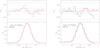 |
Fig. C.1. Same as the right panel of Fig. 2 for emission in the eastern (left panel) and western (right panel) parts of the line of nodes. |
All Tables
Zeeman parameters, frequencies, and Einstein coefficients of CN transitions that are relevant to ALMA polarisation measurements.
All Figures
|
Fig. 1. Left panel: integrated intensity map of the CN (N = 2−1, J = 3/2−1/2, F = 5/2−3/2) hyperfine transition around TW Hya. We also indicate the line of nodes of the disc at a position angle of 240° and the location of the strongest CN emission peak that was used in the polarisation analysis (see text). Right panel: continuum and polarised 226 GHz emission of the TW Hya disc. The colour scale is the total intensity dust emission. The contours, drawn at 3 and 4σ, are the linear polarisation, and the white-line segments indicate the electric vector polarisation angle. |
| In the text | |
|
Fig. 2. Total intensity (I, bottom panel) and circular polarisation (V, top panel) CN spectra. The 1σ and 3σ limits are indicated by the short and long dashed lines, respectively. Left panel: spectra stacking the nine strongest CN N = 2−1 hyperfine components that we extracted at the position of the strongest emission peak. The 1σ limit corresponds to a magnetic field strength |Bz| = 2.7 mG, for which the V-spectrum is indicated in red. The effective line width is 0.45 km s−1. The apparent non-zero baseline in the Stokes I spectrum is due to the contribution to the stacked spectrum of hyperfine components that occur within 1.5 km s−1 of each other. Middle panel: azimuthally averaged spectra obtained by stacking the two strongest CN hyperfine components in our data that are not significantly blended. The rms limit corresponds to a magnetic field strength |Bz| = 0.8 mG, for which the V-spectrum is indicated in red. The effective line width is 0.45 km s−1. Beyond +0.5 km s−1, the spectrum is affected by a blend with a neighbouring hyperfine component. Right panel: similar to the middle panel, but only for emission along the line of nodes (see text). Here the signature of a toroidal field would be strongest. The fractional rms reached on the V-spectrum is 0.33%. The rms limit corresponds to a magnetic field strength |B| = 2.6 mG, for which the V-spectrum is indicated in red. This corresponds to a toroidal field strength limit of |Bϕ| < 30 mG. The effective line width is 0.5 km s−1. |
| In the text | |
|
Fig. 3. Vertical magnetic field strength (Bz) from accretion disc models, compared with the 1σ limit obtained in our ALMA observations (Bz < 0.8 mG, indicated by the arrow). The solid line is the T Tauri model from Shu et al. (2007). The dotted line is the maximum field strength Bz, max from Okuzumi et al. (2014), taking a magnetic field strength at the outer edge of the disc (Rout = 230 au) of B∞ = 25 μG. The red long dashed line assumes B∞ = 1 mG, which corresponds to the field strength measured in proto-stellar cores and dense parts of molecular clouds, and it includes efficient advection with D = 0.025 (see text). At R < 230 au, the latter two models are identical. The solid circle shows the surface magnetic field measured on TW Hya (e.g., Sokal et al. 2018). |
| In the text | |
|
Fig. B.1. Total intensity (I, bottom panel) and circular polarisation (V, top panel) spectra for all detected CN(2−1) hyperfine components. The spectra are extracted at the position of the strongest emission peak. The figures are labelled with the component rest frequency as determined using line fitting. The 1σ (short dashed) and 3σ (long dashed) limits are indicated. The 1σ limit magnetic field values are indicated in the figure, and we also present the V-spectrum for this field strength in red. Three of the components are so close in frequency that they are presented in a single panel. |
| In the text | |
|
Fig. C.1. Same as the right panel of Fig. 2 for emission in the eastern (left panel) and western (right panel) parts of the line of nodes. |
| In the text | |
Current usage metrics show cumulative count of Article Views (full-text article views including HTML views, PDF and ePub downloads, according to the available data) and Abstracts Views on Vision4Press platform.
Data correspond to usage on the plateform after 2015. The current usage metrics is available 48-96 hours after online publication and is updated daily on week days.
Initial download of the metrics may take a while.