| Issue |
A&A
Volume 624, April 2019
|
|
|---|---|---|
| Article Number | A119 | |
| Number of page(s) | 6 | |
| Section | The Sun | |
| DOI | https://doi.org/10.1051/0004-6361/201935281 | |
| Published online | 22 April 2019 | |
Zebra-stripe sources in the double-plasma resonance model of solar radio zebras
1
Astronomical Institute of the Czech Academy of Sciences, Fričova 298, 251 65 Ondřejov, Czech Republic
e-mail: This email address is being protected from spambots. You need JavaScript enabled to view it.
2
St.-Petersburg State University, St.-Petersburg 198504, Russia
3
St.-Petersburg branch of Special Astrophysical Observatory, 196140 St.-Petersburg, Russia
Received:
15
February
2019
Accepted:
14
March
2019
Abstract
Context. Radio bursts with fine structures are used in diagnostics of solar flare plasmas, of which zebra structures are the most important. However, there is still a debate about their origin.
Aims. The most probable model of zebras is that based on double-plasma resonance (DPR) instability. The paper wants to contribute to a verification of this model.
Methods. We used analytical methods.
Results. We studied the DPR model in two scenarios: a model with the zebra-stripe sources in a single loop and a model with the zebra-stripe sources moving through a fan of magnetic field lines. In the first case, we found several new relations among the parameters of zebra stripes and their sources, which can be used to analyze observed zebras and thus to verify if the zebra is generated according to the DPR model. These relations were derived for the zebra-stripe sources distributed along the loop and also for those having some extent in the loop radius. In the scenario with the moving zebra-stripe sources, we determined the parameters of the 14 December 2006 zebra and estimated a change of the ratio of magnetic field and density scales causing the change of zebra-stripe frequencies. In this case we found that this zebra can be also explained in the model with the zebra-stripe sources in a single loop. Both the interpretations are discussed.
Key words: Sun: flares / Sun: radio radiation
© ESO 2019
1. Introduction
Fine structures of solar radio bursts contain important information about processes of particle acceleration, particle dynamics, and emission mechanisms (Fleishman et al. 1994). Zebra patterns (ZP) are one example of these structures. Their observed parameters and mechanisms are described in many papers (Slottje 1972; Kuijpers 1975; Zheleznyakov & Zlotnik 1975; Chernov 1976, 1990, 2011; LaBelle et al. 2003; Kuznetsov 2005; Bárta & Karlický 2006; Ledenev et al. 2006; Tan 2010; Karlický 2013, 2014; Zlotnik 2013; Tan et al. 2014; Chernov et al. 2014, 2018). The most probable mechanism that generates zebras is that with the double-plasma resonance (DPR) instability (Kuijpers 1975, 1980; Zheleznyakov & Zlotnik 1975; Mollwo 1983, 1988; Winglee & Dulk 1986; Yasnov & Karlický 2004; Kuznetsov & Tsap 2007; Chen et al. 2011; Karlický & Yasnov 2015; Yasnov et al. 2016, 2017; Benáček et al. 2017).
In this model, the upper-hybrid waves are generated by the DPR instability at locations in the solar atmosphere, where the DPR condition is fulfilled, i.e.,
 (1)
(1)
where fc, fUH, and fp are the electron-cyclotron, upper-hybrid, and plasma frequencies, and s is the gyro-harmonic number. These upper-hybrid waves are then transformed to observed radio waves on the same frequency (the emission on the fundamental frequency) or on its double frequency (the emission on the harmonic frequency).
In Karlický & Yasnov (2015), we considered the relation for the plasma density n and magnetic field B in the form
 (2)
(2)
 (3)
(3)
where h is the position along a part of the loop (the height in the vertically oriented part of the loop), n0 and B0 are the density and magnetic field in some reference position in the loop, and Ln and Lb are density and magnetic field scales. In this paper, we presented the method to determine the gyro-harmonic numbers of specific zebra stripes and the generalized scale
 (4)
(4)
where R is Lb/Ln.
Within the DPR model of zebras there are two scenarios of the zebra-stripes generation: in a single loop (Zheleznyakov & Zlotnik 1975; Zlotnik 2013; Karlický & Yasnov 2015, 2018a,b) and in a fan of magnetic field lines, where the region of zebra-stripes generation moves to neighboring magnetic field lines (Chen et al. 2011).
In this paper, we analyze both these scenarios in detail. We present some new relations among the parameters of zebra stripes that should be fulfilled for the zebra stripes generated according to the model with DPR instability. Thus, these relations can help us recognize if the observed zebra is generated by DPR instability or by some other mechanisms. In the model with the zebra-stripe sources in a single loop we estimate their dimensions and observed number of these sources. Then we consider the zebra scenario with the zebra-stripe sources in a fan of magnetic field lines. This scenario was proposed and used in the interpretation of the 14 December 2006 zebra observed by Chen et al. (2011). Using our method, we carry out an additional analysis of the 14 December 2006 zebra. In a simple model of the scenario by Chen et al. (2011), we estimate a change of the ratio of magnetic field and density scales causing the change of zebra-stripe frequencies. Then we show that this zebra can be also interpreted in the model with the zebra-stripe sources in the single loop. Results of the both interpretations of the 14 December 2006 zebra are discussed.
The paper is organized as follows: in Sect. 2 we analyze zebras in a single loop and in Sect. 3 zebras in a fan of magnetic field lines. The conclusions are summarized in Sect. 4.
2. Zebra-stripe sources in a single loop
2.1. Zebra-stripe sources distributed along the loop
Using the relations (1)–(3), and the relations ![Mathematical equation: $ f_{\mathrm{pe}}^2[\rm{MHz}] = C_{\mathrm{n}} n[\rm{cm}^{-3}] $](/articles/aa/full_html/2019/04/aa35281-19/aa35281-19-eq5.gif) and
and ![Mathematical equation: $ f_{\mathrm{ce}}^2[\rm{MHz}] = C_{\mathrm{b}} B^2[\rm{G}] $](/articles/aa/full_html/2019/04/aa35281-19/aa35281-19-eq6.gif) , where Cn = 8.1 × 10⁻⁵ and Cb = 2.82, the DPR condition can be expressed as
, where Cn = 8.1 × 10⁻⁵ and Cb = 2.82, the DPR condition can be expressed as
 (5)
(5)
From this, we computed the distance h of the zebra-stripe source with the gyro-harmonic number s along the loop as
 (6)
(6)
Then, the magnetic field in the zebra-stripe source with the gyro-harmonic number s1 (which corresponds to the zebra stripe with the lowest frequency) is written as
 (7)
(7)
Then the relation between n0 and B0 is
 (8)
(8)
Ratio of zebra-stripe frequencies. The upper-hybrid frequency of the zebra stripe with the gyro-harmonic number s (i.e., the zebra-stripe frequency for the emission on the fundamental frequency) is as follows:
 (9)
(9)
Using the relation for the distance hs (relation (6)) we write
 (10)
(10)
When we use the relation (8) then we have
 (11)
(11)
As seen in this relation the frequency  does not depend on n0 and B0. It depends only on B(s1) and R.
Finally, the ratio of the upper-hybrid frequencies for the gyro-harmonic numbers s to s + n is
 (12)
(12)
2.2. Zebra-stripe sources in two-dimensional loop
In this case the plasma density and magnetic field are expressed not only depending on the distance along the loop h, but also on the loop radius r as
 (13)
(13)
 (14)
(14)
where Lnh, Lbh, Lnr, and Lbr are the scales along and across the loop. The values Lnh and Lbh correspond to Ln and Lb in the relations (2) and (3), respectively. We note that these relations only approximately describe a real loop. They can be used in the cases when the length of the region, where the zebra is generated, is much shorter than Lbh.
To simplify the following relations we write Lnr = 1. Because we take Lnr as the half-width of the loop a, this means that all spatial scales and distances in the following relations are expressed in the unit of the loop half-width a.
We now derive the coordinates of the layers, where the condition for the DPR instability (the relation (1)) is fulfilled. Similar to the previous paragraph, the DPR condition can be rewritten as
 (15)
(15)
This condition needs to be fulfilled at the layer with constant plasma density and simultaneously with the constant magnetic field. Thus, using the relation (13), for the constant plasma density n = const we can write
 (16)
(16)
Now putting this relation into relation (14), we have
 (17)
(17)
Thus, the constant magnetic field is if
 (18)
(18)
i.e., if
 (19)
(19)
We note that this condition gives the zebra stripes with the zero frequency width. However, owing to the non-zero bandwidth of observed zebra stripes some small deviation from this condition still gives a resonance. If this deviation increases then there are always some short DPR layers close to the loop axis, but the emitting area of the zebra-stripe sources is small; see the analysis in Karlický & Yasnov (2018a).
Using the resonance condition (15), we can finally write the coordinates (r, h) of the layers where the zebra stripes are generated as
![Mathematical equation: $$ \begin{aligned} r = \sqrt{\frac{L_{\rm br}^2 \left[ h + L_{\rm nh} \ln \left( \frac{C_{\rm b}(s^2 -1) B_0^2 \exp {^{-\frac{2 h}{L_{\rm br}^2 L_{\rm nh}}}}}{C_{\rm n} n_0}\right) \right]}{(2 - L_{\rm br}^2) L_{\rm nh}}}, \end{aligned} $$](/articles/aa/full_html/2019/04/aa35281-19/aa35281-19-eq23.gif) (20)
(20)
and
![Mathematical equation: $$ \begin{aligned} h = \frac{L_{\rm nh} L_{\rm bh}\left[r^2 + \ln \left( \frac{C_{\rm b}(s^2 -1) B_0^2 \exp {^{-\frac{2 r^2}{L_{\rm br}^2}}}}{C_{\rm n} n_0}\right) \right]}{2 L_{\rm nh} - L_{\rm bh}}\cdot \end{aligned} $$](/articles/aa/full_html/2019/04/aa35281-19/aa35281-19-eq24.gif) (21)
(21)
The derivative dh/dr in this case is dh/dr = −2 Lnhr, which means that it does not depend on s and h and also that the points with the same derivative are located at the same distance r from the loop axis. The distances of the points along the loop that have the same derivative for two different gyro-harmonic numbers s and s + n can be expressed as
 (22)
(22)
or in the form
 (23)
(23)
where the relation (19) is used. This means that this distance does not depend not on h and r, and in the later form does not depend on the density scales.
The value of Lbr can be determined from Lnb, where the density scale in the vertically oriented part of the loop can be expressed as Lnh = 50T[K]/a (the gravitational height scale (Priest 2014) in units of the loop half-width a).
Because the centers of the emitting DPR layers are found at the same distance from the loop axis r and the distance between centers along the loop does not depend on r, the ratio of the scales of the magnetic field and density along the loop can be expressed in dependence of Lnb as
 (24)
(24)
Also the scale Lbr can be expressed in dependance on Lnb as
 (25)
(25)
2.3. Dimensions of DPR layers and their observednumber
In accordance with the relation (17) in Karlický & Yasnov (2018a), the length of the emitting region along the loop axis (Fig. 1) is
 (26)
(26)
where Θmax is the emission escaping angle, which for the emission on the fundamental frequency can be expressed as (Yasnov et al. 2017)
Then the length of this region perpendicular to the observer is (Fig. 1)
 (27)
(27)
As seen in these relations, decreasing the loop radius r, the length dh decreases faster than dl.
We now compute the ratio of the distances between the zebra-stripe sources with the gyro-harmonic numbers s and s + 1 (modified by the angle to observer  ) dhs and dl for the zebras presented in the paper by Karlický & Yasnov (2018b). These zebras were mainly observed in the decimeter wavelength range with the harmonic numbers from 15 to 45 and Lnb from 0.2 to 1.1. Calculations show that this ratio is very weakly dependent on the harmonic number s. Therefore, as an example in Fig. 2 we present this ratio for the harmonic number s = 30. The radius of the loop is taken as a = 1 Mm and Lnh = 50T[K]/a (for the temperature T = 2 × 10⁴K assumed for the decimetric zebras). For r = 1 it means that in the length of the emitting region there can be 5 to 25 centers of DPR layers.
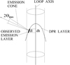 |
Fig. 1. Scheme showing the DPR and emission layers, emission cone, and dh and dl in the loop. |
Figure 3 is the same as Fig. 2, but for metric zebras. In Fig. 3, in accordance with the zebra parameters presented in Karlický & Yasnov (2018b), we take Lnb = 0.5 – 1.8 and s = 40, the temperature as T = 2 × 10⁶ K and the loop radius a = 2 Mm. As shown in this figure, for metric zebras the number of emitting centers per emitting region can be up to several hundreds.
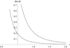 |
Fig. 2. Ratio of the distance between emitting layers dhs with s and s + 1 and the length of the layer dl for T = 2 × 10⁴ K. The radius of the loop is a = 1 Mm and s = 30. The lower curve represents Lnb = 0.2 and the upper curve represents Lnb = 1.1. |
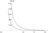 |
Fig. 3. Ratio of the distance between emitting layers dhs with s and s + 1 and the length of the layer dl for T = 2 × 10⁶ K. The radius of the loop is a = 2 Mm and s = 40. The lower curve indicates Lnb = 0.5 and the upper curve indicates Lnb = 1.8. |
We now consider an effect of the curvature of the loop having its main radius Rc. In this case dl can be expressed as
Then, similar to the previous cases without the loop curvature Rc, we compute the ratio dhs/dl for the same parameters, except Rc = 3 for decimetric zebras and Rc = 50 for metric zebras. The results for the decimetric zebras are shown in Fig. 4. As seen in this case, for r = 1 the number of emitting DPR centers cannot be greater than 14.
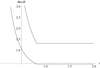 |
Fig. 4. Ratio of the distance between emitting layers dhs with s and s + 1 and the length of the layer dl for T = 2 × 10⁴ K. The radius of the loop is a = 1 Mm and s = 30. The main loop radius is Rc = 3. The lower curve indicates Lnb = 0.2 and the upper curve indicates Lnb = 1.1. |
The results for metric zebras are shown in Fig. 5. In this case, the distance between the emitting layers is greater than the possible emitting region. Thus, for small distances (r < 0.18) it is possible to observe only one DPR center. Namely, if dhs/dl > 1, then only one layer is visible. But in reality, we observe many zebra stripes. Therefore, in the metric range, zebra emission most likely occurs at the second harmonic of the upper hybrid frequency. In this case the emission escape cone is
 (28)
(28)
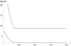 |
Fig. 5. Ratio of the distance between emitting layers dhs with s and s + 1 and the length of the layer dl for T = 2 × 10⁶ K. The radius of the loop is a = 2 Mm and s = 40. The main loop radius Rc = 50. The lower curve represents Lnb = 0.5 and the upper curve represents Lnb = 1.8. |
Then, for example for s = 50, the angle Θmax increases 50 times comparing to the case with the emission on the fundamental frequency. Thus, for the second harmonic the zebra emission is possible in almost all directions. In this case, the area of possible emission increases substantially, and the number of emitting layers increases accordingly.
3. Zebra-stripe sources moving in fan of magnetic field lines
This model was proposed by Chen et al. (2011) based on their observations of the 14 December 2006 zebra. In this model zebra stripes are generated in a post-flare loop system and their sources move through a fan of magnetic field lines; see the scenario in Fig. 14 in their paper. These authors estimated a displacement of the zebra source centroid as about 6.2 Mm. They also proposed that locations of the DPR levels can also change owing to a change of the parameters and locations of the hot anisotropic electrons generating the upper-hybrid waves and thus the observed electromagnetic waves. During zebra source motion across magnetic field lines, which is caused by a formation of the unstable electron distribution subsequently in new and new neighboring magnetic field lines, plasma parameters change and thus cause frequency variations of the zebra stripes.
This model in its simplest form (i.e., when only a motion of zebra source across the magnetic field lines is considered) can be expressed as follows: We take a set of vertically oriented parts of loops arrayed in the direction of the zebra source motion. This array of loops is considered as a part of the post-flare loop system. Another possibility is to consider a very broad loop, where the loop parameters change with the loop radius. However, in the following we assume the mentioned loop array. In all loops in the array, the density and magnetic field are taken according to the relations (2) and (3), where the same parameter n0 is assumed. The parameter B0 depends on n0; see relation (8). The frequency of the zebra stripe with the lowest frequency s1 is given by B(s1) (relation (11)). The key parameter for other frequencies and heights of the zebra-stripe sources is the parameter R = Lb/Ln = 2Lnb/(2 + Lnb). Only this parameter R or Lnb is assumed to be changed in loops in the direction of the zebra source motion and thus explains the variations of zebra-stripe frequencies. In each loop of this set, the zebra stripes are generated at the layers where the density and simultaneously also the magnetic field are constant. Thus, for each loop the same relations as derived for the zebra in a single loop can be used. Generally, changes of the plasma density and magnetic field through such a loop array are arbitrary, but in our case they need to be continuous owing to continuous frequency variations of zebra stripes. This corresponds to the idea of a very broad loop mentioned above.
We now use this simple model for the 14 December 2006 zebra. Firstly, from Chen et al. (2011) we take the frequencies of the zebra stripes No. 1 and No. 6 at two moments: T1 = 22:40:07.2 UT (see small solid box in Fig. 6 in Chen et al. 2011) and T2 = 22:40:06.9 UT, see Table 1. Then, using the method described by Karlický & Yasnov (2015) we determine the parameters s1, Lnb at T1 = 22:40:07.2 UT. The resulting s1 and Lnb are s1 = 12.7 and Lnb = 0.225 and corresponding R = 0.2024 (Table 1). The error of these values is about 7 per cent. The gyro-harmonic number s1 is that of the zebra stripe with the lowest frequency, which is the zebra stripe No. 6 in Chen et al. (2011). Therefore our gyro-harmonic number agrees to that determined by Chen et al. (2011). We note that the gyro-harmonic number need not be necessarily an integer number; see the paper by Benáček & Karlický (2018). The plasma density and magnetic field in the zebra-stripe source with s1 = 12.7 are n = 1.97 × 1010 cm−3 and B = 35.58 G, respectively (Table 1). Then assuming n0 as 2.5 × 1010 cm−3 and Ln = 1.4 × 1010 cm from Chen et al. (2011) we obtain B0 as 117.38 G and the distances along the loop as 17.8 Mm for the zebra stripe No. 1 and 33.7 Mm for that of No. 6. Thus the difference in positions of these sources is 15.9 Mm, which agrees with the value (about 20 Mm) estimated in Chen et al. (2011).
Parameters of two zebra-stripe sources of the 14 December 2006 zebra.
We now estimate the parameters in the loop, where the moving zebra source was at T2 = 22:40:06.9 UT. We assume the same density n0 = 2.5 × 1010 cm−3 as at T1, which gives B0 = 86.2 G. The value B(s1) follows from the lowest frequency at this time as B(s1) = 36.56 G. Then varying R we find the fit with the frequency of the zebra stripe No. 1 for R = 0.2178, i.e., for Lnb = 0.244 (Table 1). Finally, taking Ln = 1.4 × 1010 cm we estimate distances of the zebra sources No. 1 and No. 6 from the reference level (see Table 1).
When we compare R at both these times, we can see that R changes from 0.2178 at 22:40:06.9 UT to 0.2024 at 22:40:07.2 UT, and Lnb from 0.244 at 22:40:06.9 UT to 0.225 at 22:40:07.2 UT. We also see that positions of zebra-stripe sources along the loops in the loop array change. Just these positional changes of zebra-stripe sources along the loops in the loop array enable us to explain the zebra observations in the zebra model with the zebra-stripe sources in a single loop. Namely, when we define the position of the zebra source centroid as the sum of positions of zebra-stripe sources No. 6 and No. 1 divided by two, then the zebra centroid position at T2 is 17.5 Mm and at T1 is 25.75 Mm. Therefore the displacement along the loop is 8.25 Mm. When the observer looks on this displacement with the angle between the direction to observer and the loop axis 48° then the observed displacement is 6.2 Mm. This angle appears to be compatible with the magnetic field lines obtained by the nonlinear force-free field extrapolation presented in Fig. 12 in Chen et al. (2011). Thus, analyzing the 14 December 2006 zebra observations in the model with the zebra-stripe sources moving in a fan of magnetic field lines, we find that these observations can be also explained in the scenario with the zebra-stripe sources in a single loop.
Although both models can explain the 14 December 2006 zebra, they are not without problems. The model with the zebra-stripes sources moving through a fan of magnetic field lines requires a loop system with very similar parameters. But the most problematic aspect of this model is the demand of continuous and spatially changed injection of electrons subsequently into new and new neighboring magnetic field lines. On the other hand, in the model with the zebra-stripe sources in a single loop we still do not know how to explain the observed change of loop parameters in a very short time interval of 0.3 s. It looks as though the only possible candidate is the standing magnetosonic wave as described in Yu et al. (2016). Maybe, there are also some further possibilities or combinations of these possibilities. For example, a single loop with the zebra-stripe sources can move or change its orientation and thus change its plasma parameters and cause the observed changes. However, the velocity of a loop should be slower than the local Alfvén velocity, which in the case of the 14 December 2006 zebra is estimated as vA = 550–910 km s−1. This is much lower velocity than the velocity of the zebra source centroid estimated in Chen et al. (2011), who found ∼0.1 c, where c is the light speed. Another process that can influence the zebra-stripe frequency is a fast change of the “temperature” of the hot anisotropic electrons, which can change the ratio of the upper-hybrid and electron-cyclotron frequency for the maximum of the growth rate of the upper-hybrid waves (see Fig. 7 in Benáček & Karlický 2018).
4. Conclusions
In this paper we studied the relations among the parameters of zebra stripes and their sources within the DPR model in two scenarios: zebra-stripe sources in a single loop and zebra-stripe sources moving through a fan of magnetic field lines. These relations can be used to verify if the observed zebra is generated by the DPR instability or by some other mechanisms.
For the zebras generated in the single loop, several new relations were found. For example, in our model with the exponential dependencies of the density and magnetic field, all frequencies of the zebra stripes depend only on the magnetic field in the zebra-stripe source with the lowest gyro-harmonic number s1 and R. Furthermore, the centers of the DPR emitting surfaces are distributed along the loop with the same distance from the loop axis. The distance between these centers does not depend on the distance h (height in the vertically oriented part of the loop) and the radius r.
We also found the relation between the magnetic field and plasma density at the reference level in the considered loop. We also derived the ratio of the magnetic field and density scales, in the both height and radius directions. Numerical values of the distances between centers of the DPR layers are given under the assumption that decimeter zebras occur in the chromosphere with the temperature of 2 × 10⁴ K and the meter zebras in the corona with the temperature of about 2 × 10⁶ K. We estimated the dimensions of the DPR layers and their possible visible numbers in the cases with and without the loop curvature.
We carried out an additional analysis of the 14 December 2006 zebra observed by Chen et al. (2011). With our method we confirmed the main parameters of this zebra as evaluated by Chen et al. (2011). Considering the scenario with moving zebra-stripe sources in its simplest model we estimated the change of the ratio of the magnetic field and density scales explaining the frequency variation of zebra stripes in this zebra. Although this model can explain the zebra, there are some problems with this model. Owing to the continuity of zebra-stripe frequencies, the model requires a set of loops with very similar parameters. But the most problematic aspect of this model is the demand of continuous and spatially changed injection of electrons subsequently into new and new neighboring magnetic field lines. We also recognize that a change of the temperature of the hot anisotropic electrons can change the location of the DPR layer and thus the frequency of the zebra stripes. Furthermore, in analyzing the zebra in the model with the zebra-stripe sources moving through a fan of magnetic field lines we found that this zebra can be also explained in the zebra model with the zebra-stripe sources in a single loop. Although the model with the zebra in a single loop offers us a simple explanation, the question arises of what causes the needed change of loop parameters in a very short time interval of 0.3 s. We propose the standing magnetosonic wave, but this needs to be verified by a much more sophisticated model, which is beyond a scope of this paper.
Acknowledgments
The authors thank the referee for constructive comments that improved the article. M. Karlický acknowledges support from Grants 17-16447S, 18-09072S and 19-09489S of the Grant Agency of the Czech Republic. L.V. Yasnov acknowledges support from Grants 18-29-21016-mk and 18-02-00045 of the Russian Foundation for Basic Research.
References
- Bárta, M., & Karlický, M. 2006, A&A, 450, 359 [NASA ADS] [CrossRef] [EDP Sciences] [Google Scholar]
- Benáček, J., & Karlický, M. 2018, A&A, 611, A60 [NASA ADS] [CrossRef] [EDP Sciences] [Google Scholar]
- Benáček, J., Karlický, M., & Yasnov, L. V. 2017, A&A, 598, A106 [NASA ADS] [CrossRef] [EDP Sciences] [Google Scholar]
- Chen, B., Bastian, T. S., Gary, D. E., & Jing, J. 2011, ApJ, 736, 64 [NASA ADS] [CrossRef] [Google Scholar]
- Chernov, G. P. 1976, Sov. Ast., 20, 449 [NASA ADS] [Google Scholar]
- Chernov, G. P. 1990, Sol. Phys., 130, 75 [NASA ADS] [CrossRef] [Google Scholar]
- Chernov, G. 2011, Fine Structure of Solar Radio Bursts (Berlin: Springer) [Google Scholar]
- Chernov, G. P., Yan, Y.-H., & Fu, Q.-J. 2014, Res. Astron. Astrophys., 14, 831 [NASA ADS] [CrossRef] [Google Scholar]
- Chernov, G. P., Fomichev, V. V., & Sych, R. A. 2018, Geomag. Aeron., 58, 394 [CrossRef] [Google Scholar]
- Fleishman, G. D., Stepanov, A. V., & Yurovsky, Y. F. 1994, Space Sci. Rev., 68, 205 [NASA ADS] [CrossRef] [Google Scholar]
- Karlický, M. 2013, A&A, 552, A90 [NASA ADS] [CrossRef] [EDP Sciences] [Google Scholar]
- Karlický, M. 2014, A&A, 561, A34 [NASA ADS] [CrossRef] [EDP Sciences] [Google Scholar]
- Karlický, M., & Yasnov, L. V. 2015, A&A, 581, A115 [NASA ADS] [CrossRef] [EDP Sciences] [Google Scholar]
- Karlický, M., & Yasnov, L. 2018a, A&A, 618, A60 [NASA ADS] [CrossRef] [EDP Sciences] [Google Scholar]
- Karlický, M., & Yasnov, L. V. 2018b, ApJ, 867, 28 [NASA ADS] [CrossRef] [Google Scholar]
- Kuijpers, J. 1980, in Radio Physics of the Sun, eds. M. R. Kundu, & T. E. Gergely, IAU Symp., 86, 341 [NASA ADS] [CrossRef] [Google Scholar]
- Kuijpers, J. M. E. 1975, PhD thesis, Utrecht, Rijksuniversiteit, The Netherlands [Google Scholar]
- Kuznetsov, A. A. 2005, A&A, 438, 341 [NASA ADS] [CrossRef] [EDP Sciences] [Google Scholar]
- Kuznetsov, A. A., & Tsap, Y. T. 2007, Sol. Phys., 241, 127 [NASA ADS] [CrossRef] [Google Scholar]
- LaBelle, J., Treumann, R. A., Yoon, P. H., & Karlický, M. 2003, ApJ, 593, 1195 [NASA ADS] [CrossRef] [Google Scholar]
- Ledenev, V. G., Yan, Y., & Fu, Q. 2006, Sol. Phys., 233, 129 [NASA ADS] [CrossRef] [Google Scholar]
- Mollwo, L. 1983, Sol. Phys., 83, 305 [NASA ADS] [CrossRef] [Google Scholar]
- Mollwo, L. 1988, Sol. Phys., 116, 323 [NASA ADS] [Google Scholar]
- Priest, E. 2014, Magnetohydrodynamics of the Sun (UK: Cambridge University Press) [Google Scholar]
- Slottje, C. 1972, Sol. Phys., 25, 210 [NASA ADS] [CrossRef] [Google Scholar]
- Tan, B. 2010, Astrophys. Space Sci., 325, 251 [NASA ADS] [CrossRef] [Google Scholar]
- Tan, B., Tan, C., Zhang, Y., Mészárosová, H., & Karlický, M. 2014, ApJ, 780, 129 [NASA ADS] [CrossRef] [Google Scholar]
- Winglee, R. M., & Dulk, G. A. 1986, ApJ, 307, 808 [NASA ADS] [CrossRef] [Google Scholar]
- Yasnov, L. V., & Karlický, M. 2004, Sol. Phys., 219, 289 [NASA ADS] [CrossRef] [Google Scholar]
- Yasnov, L. V., Karlický, M., & Stupishin, A. G. 2016, Sol. Phys., 291, 2037 [NASA ADS] [CrossRef] [Google Scholar]
- Yasnov, L. V., Benáček, J., & Karlický, M. 2017, Sol. Phys., 292, 163 [NASA ADS] [CrossRef] [Google Scholar]
- Yu, S., Nakariakov, V. M., & Yan, Y. 2016, ApJ, 826, 78 [NASA ADS] [CrossRef] [Google Scholar]
- Zheleznyakov, V. V., & Zlotnik, E. Y. 1975, Sol. Phys., 44, 461 [NASA ADS] [CrossRef] [Google Scholar]
- Zlotnik, E. Y. 2013, Sol. Phys., 284, 579 [NASA ADS] [CrossRef] [Google Scholar]
All Tables
All Figures
|
Fig. 1. Scheme showing the DPR and emission layers, emission cone, and dh and dl in the loop. |
| In the text | |
|
Fig. 2. Ratio of the distance between emitting layers dhs with s and s + 1 and the length of the layer dl for T = 2 × 10⁴ K. The radius of the loop is a = 1 Mm and s = 30. The lower curve represents Lnb = 0.2 and the upper curve represents Lnb = 1.1. |
| In the text | |
|
Fig. 3. Ratio of the distance between emitting layers dhs with s and s + 1 and the length of the layer dl for T = 2 × 10⁶ K. The radius of the loop is a = 2 Mm and s = 40. The lower curve indicates Lnb = 0.5 and the upper curve indicates Lnb = 1.8. |
| In the text | |
|
Fig. 4. Ratio of the distance between emitting layers dhs with s and s + 1 and the length of the layer dl for T = 2 × 10⁴ K. The radius of the loop is a = 1 Mm and s = 30. The main loop radius is Rc = 3. The lower curve indicates Lnb = 0.2 and the upper curve indicates Lnb = 1.1. |
| In the text | |
|
Fig. 5. Ratio of the distance between emitting layers dhs with s and s + 1 and the length of the layer dl for T = 2 × 10⁶ K. The radius of the loop is a = 2 Mm and s = 40. The main loop radius Rc = 50. The lower curve represents Lnb = 0.5 and the upper curve represents Lnb = 1.8. |
| In the text | |
Current usage metrics show cumulative count of Article Views (full-text article views including HTML views, PDF and ePub downloads, according to the available data) and Abstracts Views on Vision4Press platform.
Data correspond to usage on the plateform after 2015. The current usage metrics is available 48-96 hours after online publication and is updated daily on week days.
Initial download of the metrics may take a while.