| Issue |
A&A
Volume 624, April 2019
|
|
|---|---|---|
| Article Number | A61 | |
| Number of page(s) | 14 | |
| Section | Cosmology (including clusters of galaxies) | |
| DOI | https://doi.org/10.1051/0004-6361/201834343 | |
| Published online | 12 April 2019 | |
Fast and easy super-sample covariance of large-scale structure observables⋆
1
Département de Physique Théorique and Center for Astroparticle Physics, Université de Genève, 24 quai Ernest Ansermet, 1211 Geneva, Switzerland
e-mail: This email address is being protected from spambots. You need JavaScript enabled to view it.
2
Institut d’Astrophysique Spatiale, CNRS (UMR8617) and Université Paris-Sud 11, Bâtiment 121, 91405 Orsay, France
Received:
28
September
2018
Accepted:
15
February
2019
Abstract
We present a numerically cheap approximation to super-sample covariance (SSC) of large-scale structure cosmological probes, first in the case of angular power spectra. No new elements are needed besides those used to predict the considered probes, thus relieving analysis pipelines from having to develop a full SSC modeling, and reducing the computational load. The approximation is asymptotically exact for fine redshift bins Δz → 0. We furthermore show how it can be implemented at the level of a Gaussian likelihood or a Fisher matrix forecast as a fast correction to the Gaussian case without needing to build large covariance matrices. Numerical application to a Euclid-like survey show that, compared to a full SSC computation, the approximation nicely recovers the signal-to-noise ratio and the Fisher forecasts on cosmological parameters of the wCDM cosmological model. Moreover, it allows for a fast prediction of which parameters are going to be the most affected by SSC and at what level. In the case of photometric galaxy clustering with Euclid-like specifications, we find that σ8, ns, and the dark energy equation of state w are particularly heavily affected. We finally show how to generalize the approximation for probes other than angular spectra (correlation functions, number counts, and bispectra) and at the likelihood level, allowing for the latter to be non-Gaussian if necessary. We release publicly a Python module allowing the implementation of the SSC approximation and a notebook reproducing the plots of the article.
Key words: large-scale structure of Universe / galaxies: statistics / methods: data analysis / methods: analytical
The Python module is available at https://github.com/fabienlacasa/PySSC and at the CDS via anonymous ftp to cdsarc.u-strasbg.fr (130.79.128.5) or via http://cdsarc.u-strasbg.fr/viz-bin/qcat?J/A+A/624/A61
© ESO 2019
1. Introduction
The distribution of matter on large scales in the Universe is one of the main cosmological probes allowing for shading lights, for example on dark matter, dark energy, and gravity at cosmological scales. The current surveys of galaxies such as the Kilo-Degree Survey (KiDS; Hildebrandt et al. 2017) and the Dark Energy Survey (DES; Dark Energy Survey Collaboration 2018) recently provided cosmological constraints on the ΛCDM model from galaxy clustering and weak lensing, which are now competitive with constraints derived from the lensing of the Cosmic Microwave Background (CMB) and consistent with CMB primary anisotropies (for a recent comparison, see e.g., Planck Collaboration VI 2018). In the near future, large surveys such as the Large Synoptic Sky Telescope (LSST; LSST Science Collaborations 2009) and the Euclid satellite mission (Laureijs et al. 2011) will greatly improve our understanding of the structure of the Universe, the nature and the properties of dark energy, the potential modification of gravity at cosmological scales, and the initial conditions of cosmological perturbations (Amendola et al. 2013).
Unlike CMB primary anisotropies, however, late-time tracers of the large-scale structures (LSS) evolved through nonlinear dynamics, and as a result, the probability distribution function (pdf) of probes such as the galaxy distribution or weak lensing by LSS is no longer Gaussian, with deviation from a Gaussian distribution increasing at smaller scales. This first means that not all the information is compressed in the two-point statistics of the considered probes. Second, this means that the covariance of statistical observables built from LSS tracers (e.g., any n-point statistics) is increased by the presence of non-Gaussian contributions; as an example, the covariance on angular power spectra will be increased by contributions from a nonvanishing trispectrum. In the present context of preparing the cosmological interpretation of forthcoming datasets, and of forecasting the expected performance of future galaxy surveys that aim at precision cosmology from LSS tracers, it is now necessary to properly take into account the non-Gaussian contribution to the covariance for any inference of cosmological parameters from LSS observables.
Among the different non-Gaussian sources to the covariance (see Lacasa 2018 for a full derivation) is the super-sample covariance (SSC), first discovered for cluster counts by Hu & Kravtsov (2003) and to which a vast amount of literature has been devoted (e.g., Takada & Hu 2013; Takada & Spergel 2014; Takahashi et al. 2014; Li et al. 2018; Chan et al. 2018; Lacasa et al. 2018; Barreira et al. 2018a,b). This additional source of cosmic variance is inherent to all galaxy surveys due to the limited portion of the Universe that is observed, both in redshift depth and in sky fraction. SSC hence comes from the nonlinear impact of density fluctuations with wavelengths greater than the survey size. These super-survey modes modulate the local observables by making the background density averaged over the survey size to be nonrepresentative (either denser or less dense than) of the averaged density in the Universe. Barring systematics, SSC is expected to be the dominant source of statistical error or cosmic variance for weak lensing (Barreira et al. 2018a) beyond the usual Gaussian covariance, although other terms may also be important for galaxy clustering (Lacasa 2018). It affects the whole set of statistical observables and correlates them. Contrary to intrasurvey sources of covariance, it can be shown that SSC cannot be reliably calibrated from the data itself or from classical simulations (Lacasa & Kunz 2017). This thus motivates the need for analytical or semi-analytical predictions of the effect, for use in the analysis of current and future galaxy surveys.
When analyzing such galaxy surveys, we usually deal with observables 𝒪i being line-of-sight integrals of the form 𝒪i = ∫dVi 𝔬i, where 𝔬i is the comoving density of the observable (including selection effects such as redshift binning) and  is the comoving volume per steradian. Then the rigorous super-sample covariance for such observables is given by (e.g., Lacasa & Rosenfeld 2016)
 (1)
(1)
In the above,  is the response of the probe which amounts how a given probe varies with changes of the background density δb. The quantity σ2(z1, z2) reads (assuming full sky here for simplicity)
 (2)
(2)
with Pm(k|z12) the linear matter cross-spectrum between redshifts z1 and z2, and j0 the spherical Bessel functions. It basically amounts to the variation in background density on a given survey volume due to super-survey modes modulations.
Computing this SSC contribution to the covariance exactly, however, becomes costly very quickly. In practice, we take advantage of the separability in redshift (e.g., Lacasa et al. 2018; Barreira et al. 2018b) to reduce the cost of a covariance evaluation to that of an angular power spectrum evaluation. However the covariance needs to be evaluated at every pair of multipoles. For future surveys doing angular power spectra analysis with ℓmax of a few thousands, this induces a 𝒪(103) slow-down of prediction pipelines, which can be increased by more orders of magnitude if we include tomography (⇒ pairs of redshift bins) and combine probes (⇒ pairs of probes).
Furthermore, an exact computation necessitates the knowledge of the probe’s response  , either through analytical means or through simulations, for every redshift and multipoles, which is a barrier for analysts not already experts in the field of SSC. It is thus desirable to have instead simpler functions, if not fixed parameters, as we will find later on, with reference ansatzs that can be easily implemented by the community.
The aim of this article is thus to present an approximation for the SSC that allows fast numerical computation and ease of use by the community, and to assess its accuracy in a forecast analysis using the Fisher matrix approach.
The article is organized as follows. Our approximation is presented in Sect. 2 for the case of angular power spectra as our statistical observables. This approximation basically abolishes the above-mentioned numerical burden, and makes the computation of the super-sample covariance matrix as fast as the computation of the involved angular power spectra. Furthermore, we show in Sect. 3 that the resulting matrix form enables fast application to common uses of the covariance (i.e., in a Gaussian likelihood or for computation of a signal-to-noise ratio, S/N, or a Fisher matrix) as a correction to the Gaussian case. Then in Sect. 4 we show numerical results validating the approximation and giving its range of applicability. Finally in Sect. 5 we generalize the approach to other statistics (number counts, correlation function, and bispectrum) and to the full likelihood, making the implementation of super-sample covariance feasible even if the likelihood is not Gaussian.
We release publicly a Python code that allows the easy implemention of SSC with our approach1.
2. Approximating the SSC
We consider the case of the angular power spectra cross-correlating two LSS tracers, A and B. In the context of galaxy surveys, these two tracers typically are galaxy clustering and galaxy shear. This can, however, be extended to other LSS tracers such as lensing of the CMB or the integrated Sachs-Wolfe (iSW) effect. The signals are observed in some redshift bins indicated with indices iz, jz, etc., and with a given width. In full generality, the redshift bins may overlap2.
We use the Limber approximation throughout the article, both for the power spectrum and the super-sample covariance. The approximation is accurate enough for the power spectrum on the range of scales of our later forecast (ℓ ≥ 50). Furthermore, it is even more adapted to super-sample covariance because SSC impacts the covariance on small scales ℓ ≳ 300, as we show in Sect. 4.
With Limber approximation, the angular power spectrum between two signals can generally be written as
 (3)
(3)
The weighting kernels  ,
,  are nonzero over the width of the redshift bin, and are expressed in units of [probe unit] ⋅ sr/(Mpc/h)3. The quantity PAB(kℓ|z) is the 3D power spectrum of the considered probe, evaluated at the Limber wavenumber kℓ = (ℓ+1/2)/r(z), with r(z) the comoving distance. Weighting kernels and power spectra for the different probes of interest (galaxy clustering and shear, CMB lensing, iSW effect) are given in Appendix A.
For an angular power spectrum, the comoving density of the observable, i.e., 𝔬AB entering Eq. (1), is  . Assuming that in Eq. (1) the responses,
  , vary slowly with redshift compared to σ2(z1, z2), we arrive at the approximation that is the basis of this article:
 (4)
(4)
where the double integrals over redshift in Eq. (1) have been approximately performed. The matrix  is the dimensionless volume-averaged (co)variance of the background matter density contrast
 (5)
(5)
with
 (6)
(6)
The quantity Rℓ is the effective relative response of the considered power spectrum. In the context of second-order perturbation theory (hereafter 2PT), the growth-only response of the matter power spectrum is  (e.g., Takada & Hu 2013), i.e.,
  . Other nonlinear terms are present, however, which increase the total response. In Appendix C we detail these terms, and present a full computation of the response. Our formalism is valid for a general scale-dependent response. In numerical applications later in this article, we test the approximation both with the full response and with the simpler ansatz Rℓ = 5 ≡ R, which is the effective value found in Appendix C.
The key point is that starting from the approximation in Eq. (4) makes the computation of the SSC for angular power spectra have the same numerical cost as the computation of the power spectra themselves.
3. Application to parameter constraints
In this section we examine the consequences for data analysis or forecasts of the SSC covariance given by Eq. (4) as an update to the covariance, i.e., the total covariance is 𝒞 = 𝒞noSSC + 𝒞SSC, where 𝒞noSSC is the sum of all other contributions to the covariance matrix.
A common statistical use of a covariance matrix, 𝒞, is to compute scalar quantities of the form3
 (7)
(7)
where the dot “⋅” stands for matrix multiplication. For example, to compute the cumulative S/N we would have X = Y = (Cℓ)ℓ = ℓmin⋯ℓmax ≡ C. In the exponent of a Gaussian likelihood, we would need X = Y = Ĉ − C(p), where Ĉ ≡ Ĉℓℓ = ℓmin⋯ℓmax is the estimated/measured power spectrum and C(p)≡(Cℓ(p))ℓ = ℓmin⋯ℓmax is the predicted power spectrum with model parameters p. Finally for Fisher forecasts, computing the Fisher matrix, Fα, β, requires X = ∂C/∂pα ≡ ∂αC and Y = ∂βC.
This last case is the primary aim of the article since it is a measure of the amount of information we have on cosmological parameters from the observables C. The Fisher matrix will be our figure of merit to gauge the quality of the approximation, with numerical results to be presented in Sect. 4.
Computing the scalar quantities given by Eq. (7) requires the inversion of the covariance matrix, 𝒞 = 𝒞noSSC + 𝒞SSC. Using the approximation Eq. (4), adding the SSC corresponds to a rank 1 update of the covariance matrix of the angular power spectrum Cℓ. Furthermore, in Appendix D, we detail the way to introduce binned power spectra in this approach, and we show that adding the SSC to the covariance of the binned spectra is also a rank 1 update of the covariance.
We thus make use of the Sherman–Morrison formula (Sherman & Morrison 1950; Bartlett 1951), which gives the impact on matrix inversion of a rank 1 update,
 (8)
(8)
where A is any n × n square matrix, and U and V are two n-dimensional vectors, and T means the transpose.
3.1. Single probe and single redshift bin
If we neglect all non-Gaussian terms except SSC, the noSSC covariance reduces to the Gaussian term which is diagonal in full sky:
 (9)
(9)
This can simplify the inversion of the noSSC covariance later on. In partial sky observations, the Gaussian covariance will not be diagonal due to mask-induced couplings between different angular scales (i.e., ℓ-to-ℓ′ couplings). It can nevertheless be made diagonal in practice by binning the power spectrum with bins wider than the typical width of the mask-induced couplings, as shown in Appendix D.
In the following we keep the covariance general throughout the derivation, and indicate when appropriate which expressions are simplified by the diagonal assumption. We also keep the same subscript, ℓ, to indicate either single multipoles or bins of multipoles.
The super-sample covariance has a separable form between the two multipoles so that we can write the total covariance as
 (10)
(10)
where V is a vector with size the number of multipoles, given by
 (11)
(11)
and Si, i is just a number. The Sherman–Morrison formula Eq. (8) then gives the inverse covariance as
 (12)
(12)
where  is a scalar.
Thus, the scalar quantity defined in Eq. (7) is given by
 (13)
(13)
where we defined the scalar
 (14)
(14)
The notation  in the above means that the assumption that the noSSC covariance matrix is diagonal has been used. In particular for Fisher matrices, SSC gives a negative correction to the noSSC case:
 (15)
(15)
with
 (16)
(16)
We finally note that all the above expressions for the impact of the SSC are easily extended to the case of binned spectra by replacing the vector Vℓ by its binned version, Vb (see Appendix D).
3.2. Multi-probe and single redshift bin
A more complex case of interest is when we have spectra of different probes sharing the same redshift bin. One example is a multi-tracer analysis for galaxy clustering at a given redshift. Another is a weak-lensing analysis splitting galaxy types (e.g., red vs. blue galaxies) to better mitigate the effect of intrinsic alignments.
In the following we illustrate this with two probes (A and B) yielding three power spectra, although the results hold straightforwardly for more probes.
The three angular power spectra are generally correlated. So even in the Gaussian case, the covariance matrix is not diagonal as a function of probes, for example, even in full sky:
 (17)
(17)
However, it remains diagonal as a function of multipoles.
Given that they share the same redshift bin, and assuming the weighting kernels to have similar enough redshift dependence within the bin, the S matrix can be assumed independent of probes :
 (18)
(18)
This property simplifies the super-sample covariance, allowing us to easily compute its impact on Fisher forecasts as we show below.
In the following we call nc the number of spectra and nℓ the number of multipoles. It now becomes useful to arrange the nc × nℓ data vector C grouping probes together before multipoles, for example with two probes A and B:
 (19)
(19)
The covariance matrix has a size (nc × nℓ)×(nc × nℓ). With C arranged as above, the covariance matrix is thus partitioned in nℓ × nℓ blocks, each of these blocks having a size nc × nc.
In the Gaussian case, in full sky or with the fsky approximation, the covariance matrix is block diagonal, and we call Gℓ these blocks of size nc × nc on the diagonal (see Appendix D for the case of binned spectra).
The formalism of Sect. 3.1 for a single probe is then easily adapted with only slight changes. We have the total covariance matrix
 (20)
(20)
where V is a nc × nℓ vector, given by
 (21)
(21)
Then the inverse covariance follows
where  is a scalar. For a block-diagonal covariance, it simplifies to
 (22)
(22)
with the inner matrix products being in the space of the nc spectra, and appropriately reduced to the case of Sect. 3.1 when nc = 1.
Thus, the scalar quantity defined in Eq. (7) is given by
 (23)
(23)
where we defined the scalar
 (24)
(24)
with again the inner matrix products in the space of the nc spectra.
Finally, the total Fisher matrix is given by the noSSC Fisher matrix plus a negative SSC correction:
 (25)
(25)
with
 (26)
(26)
3.3. Multi-probe and multiple redshift bins
A first case of interest is when we have probes in different nonoverlapping bins, or when the overlap is small enough to be neglected. This happens for instance for galaxies, cluster counts, or power spectra in sufficiently wide bins, i.e., larger than the photo-z error bars, and ≥0.1 to be larger than the width of the SSC σ2(z1, z2) (see Fig. 6 in Lacasa & Rosenfeld 2016).
In this case we can basically add up the bins independently,
 (27)
(27)
where Ii, i is given by Eq. (23). The (negative) SSC correction is
 (28)
(28)
In particular for Fisher forecasts, the (negative) SSC correction reads
 (29)
(29)
which is obtained as the sum over independent redshift bins of the SSC corrections derived for one single bin.
The second case of interest is when bins are overlapping. This happens for instance when analyzing galaxy shear, which integrates the signal from z = 0 to the sources, either alone or in combination with other probes. In that case, no simplifications can be carried out: the power spectra are correlated both as a function of multipoles and as a function of redshift bins. The covariance matrix must be built in full generality using Eq. (4), and then inverted numerically. We note that already at the Gaussian level inversion must be carried out numerically, due to the coupling between redshift bins.
3.4. Importance of SSC: an analytical rule of thumb
The importance of SSC can be gauged easily in an analytical way, if we assume a single redshift bin, and further approximate the response Rℓ to be independent of scale Rℓ ≡ R. It is important to note that this scale independent assumption is not a requirement for numerical application, and may be relaxed as is be done in Sect. 4.
In this section, we gauge the importance of SSC analytically first for the S/N, then for the Fisher constraints.
10pt
3.4.1. Impact on the signal-to-noise ratio
The S/N of a set of angular power spectra, collected in a single data vector C, is given by
 (30)
(30)
and we also introduce the noSSC version of it as
 (31)
(31)
We recall that these are cumulative S/N values obtained as a summation over multipoles up to a maximum value ℓmax. It is then a function of the maximum multipole up to which we integrate our observables. Let us also introduce the scalar quantity
 (32)
(32)
With the assumption of a single redshift bin and a scale-independent response, the scalar Y is shown to be proportional to the square of the noSSC S/N, i.e.,
 (33)
(33)
Then the total (S/N) boils down to
 (34)
(34)
It is thus obvious that the SSC decreases the S/N compared to the noSSC case as Y is by construction a positive number. The impact of the SSC is enhanced for higher values of Y, which is then an excellent indicator of its importance4.
From Eq. (33), the impact of the SSC increases for higher S/N: the higher (S/N)noSSC, the higher Y. Enlarging the set of power spectra to smaller angular scales (i.e., increasing ℓmax to higher multipoles) increases the S/N, hence the impact of the SSC. By integrating to smaller scales, the entire S/N will thus reach a plateau at an asymptotic value
 (35)
(35)
This saturation is reached when Y ∼ 1. For the case of a full sky cosmic variance-limited analysis of a single power spectrum up to a maximum multipole ℓmax, and neglecting other non-Gaussian terms, we have  . The typical angular scales above which the (S/N) starts to saturate because of the SSC is defined by Y ≃ 1. We thus find that SSC becomes important when the analysis goes up to ℓmax ≳ ℓSSC given by
 (36)
(36)
Generalizing to the case of partial sky coverage and several cosmic variance-limited probes (in the same redshift bin and neglecting other non-Gaussian terms), the analysis is affected as soon as it reaches multipoles of order
 (37)
(37)
where
 (38)
(38)
is the effective number of probes5.
Finally, if the probes are not cosmic variance-limited, for example due to the presence of shot-noise (galaxy clustering) or shape noise (weak lensing), or if other non-Gaussian covariance terms are important, then we need a full computation of the noSSC S/N accounting for these additional sources of error; the criterion for the importance of SSC is  . We note that this critical value is that of the maximum S/N with the full covariance (Eq. (35)), this plateau being the same for single- and multi-probe cases (as long as all probes have the same response R); in other words, it is the maximum amount of information that can be extracted from matter fluctuations in a finite volume of the universe with probes with a given response, regardless of the number of probes.
3.4.2. Impact on Fisher constraints
The S/N is highly impacted by SSC, because in the SSC dominated regime and with a constant Rℓ, Eq. (4) shows that Cℓ measurements are 100% correlated and thus all information is lost on the overall amplitude. However, one may question the impact on cosmological parameters, if they are sensitive to other features of the power spectrum.
We first recall Eq. (25) for the Fisher information on model parameters α and β,
 (39)
(39)
rewritten here using Y. We further introduce two angles: first, the angle θα between the vectors C and ∂αC,
 (40)
(40)
and second, the angle θαβ between ∂αC and ∂βC,
 (41)
(41)
Let us roughly interpret these angles. The second, θαβ, is easily interpreted as the noSSC correlation between the parameter α and the parameter β. The first angle, θα, can be interpreted as follows. We recall that V is proportional to the data vector C. Up to a normalization constant, C and thus V can be viewed as ∂AC, where A is the normalization of the data vector. Since angles are obtained from normalized vectors, θα is thus a measure of the noSSC correlation between the parameter α and the normalization of the data vector.
The Fisher information matrix including SSC is then conveniently expressed as a function of the noSSC Fisher matrix, the parameters Y measuring the impact of the SSC on the S/N, and the angles θα, θβ, and θαβ:
 (42)
(42)
The impact of the SSC on the Fisher matrix is driven first by the impact of the SSC on the (S/N) through Y, and then by the angles θα, θβ, and θαβ. In particular for the diagonal elements, the change of the Fisher matrix is
 (43)
(43)
This has a negative value, showing that the SSC lowers the amount of information on a given parameter.
Two conditions have to be met for the impact of the SSC to be important: Y should be greater than one, and cos2θα should be close to one. Supposing Y ≫ 1 and if θα ≠ 0, π, i.e., cos θα ≠ ±16, then the Fisher information keeps increasing with ℓmax, but at a reduced rate compared to the noSSC case, with the asymptote
 (44)
(44)
i.e., the unmarginalized error bar is increased as
 (45)
(45)
A maximum impact of the SSC is thus obtained for θα close to zero, that is when the parameter α is at the noSSC level highly correlated with the normalization of the data vector.
When we have several parameters, the situation becomes more complex and cannot be judged with only rules of thumb. For example, a parameter α may seem unaffected by SSC because cos θα ≪ 1, but it may be correlated (already at the noSSC level) with a parameter β which is affected by SSC, so that α will be affected indirectly through marginalization. Another possibility is that we have two parameters that are uncorrelated at the noSSC level, but through Eq. (42) they become correlated due to SSC ; in that case a large error on one parameter would rebound on the other, which did not happen in the noSSC case.
Summary. To decide the importance of SSC on parameter constraints, first compute the multipole above which the SSC dominated regime is entered, i.e.,
 (46)
(46)
If the analysis is restricted to scales such as ℓ ≪ ℓSSC, then it will not be affected. If the analysis enters the SSC dominated regime, then for each parameter of interest it is necessary to compute the angle
 (47)
(47)
and the (unmarginalized) error bar on parameter α is increased asymptotically as
 (48)
(48)
In the case with several cosmological parameters and/or nuisance parameters that need to be marginalized over, a full computation is necessary.
4. Numerical application to Fisher forecasts
To test the accuracy of the proposed SSC approximation, and to illustrate its impact on a cosmological analysis, we perform here an application to forecast the cosmological constraints from photometric galaxy clustering with the following specifications:
-
–
single redshift bin with a top-hat window 0.9 < z < 1, and galaxy numbers representative of Euclid: 28M galaxies in the bin, corresponding to a density of ∼2.5 gal arcmin−2;
-
–
full sky coverage and an analysis in the multipole range 50 < ℓ < 2000, in bins of constant width Δℓ = 50 (a realistic range for a conservative photometric galaxy cosmological analysis relying on a constant bias model);
-
–
flat wCDM model with fiducial cosmological parameters from Planck 2013 ΛCDM constraints (Planck Collaboration XVI 2014):

-
–
other non-Gaussian covariance terms beyond SSC are neglected.
With these specifications, we compute the galaxy angular power spectrum  using the halo model and halo occupation distribution as done in Lacasa & Rosenfeld (2016). On the one hand we find that the shot-noise level is completely negligible, so that we are signal-dominated over all the scales of interest. On the other hand, we find that the nonlinear part of the power spectrum is important on those scales, with the one-halo term dominating the two-halo term for ℓ > 800.
For the S matrix, computed following Appendix B.2, we find the value
 (49)
(49)
Following Sect. 3.4.1 and assuming a scale independent response R = 5, this translates into a knee multipole ℓSSC ∼ 360, and a plateau at S/N ∼ 250.
The cumulative S/N as a function of the maximum multipole of the analysis ℓmax is shown in Fig. 1. The (S/N) is computed with three different covariance matrices: Gaussian only, Gaussian plus SSC through Eq. (34), and Gaussian plus a full SSC computation following Lacasa & Rosenfeld (2016). We see that the Gaussian covariance matrix completely overestimates the significance of the angular power spectrum by a factor of ∼5.7 at ℓmax = 2000. However, the Si, j approximation with a constant response does recover precisely the full SSC computation over the whole multipole range with a precision better than 7%. We also see that the value of the knee multipole and the (S/N) plateau mentioned previously indeed capture the features of the full SSC curve. The Sij approximation is thus validated at the level of the S/N.
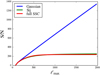 |
Fig. 1. Comparison of the cumulative S/N values up to a multipole ℓmax with different covariances: Gaussian only, with the Si, j approximation, and with a full SSC computation. |
The impact of the SSC on the cosmological parameter estimation is depicted in Figs. 2 and 3. Figure 2 shows the angle cos2θα, defined by Eq. (40), for the main cosmological parameters of the wCDM model considered here. Interestingly, all curves are significantly different from zero. Following Sect. 3.4.2, this means that all parameters are going to be significantly impacted by SSC when reaching small scales (i.e., ℓ ≳ ℓSSC). In this specific case, a value of cos2θα significantly different from zero will thus matter for an ℓmax greater than ∼400. Some parameters should be affected less (Ωbh2, Ωch2, and h), and others more (σ8, ns, and w0).
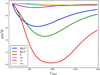 |
Fig. 2. cos2θ for each cosmological parameter as a function of the maximum multipole ℓmax. Parameters with cos2θ close to 1 are the most affected by SSC when it starts to dominate the covariance (i.e., for multipoles ℓ ≳ ℓSSC with ℓSSC 360 in this specific case). |
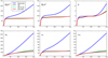 |
Fig. 3. Comparison of |

Figure 3 confirms the qualitative conclusion of Fig. 2. It shows for each cosmological parameter the square root of the Fisher element as a function of the maximum multipole ℓmax of analysis. This coefficient has an evolution with ℓmax similar to the S/N7, and its inverse is the error bar on the considered cosmological parameter when the other parameters are fixed8. As in the case of the (S/N), on large scales (ℓmax < ℓSSC) the impact of the SSC is negligible. This happens in spite of the angle cos2θα being close to one for all the parameters, simply because the impact of the SSC on the (S/N) is subdominant: Y ≪ 1. When we integrate the signal to smaller scales, however (ℓmax ≳ ℓSSC), the Gaussian covariance significantly overestimates the strength of the angular power spectrum: the Fisher elements become significantly smaller with the full covariance compared to the Gaussian case. Furthermore, the parameters most affected by SSC are indeed those that were identified in Fig. 2 (σ8, ns, and w0), although the other parameters are still significantly affected. We note that this finding is in agreement with the recent analysis of Barreira et al. (2018a) in the different case of weak lensing.
We now briefly discuss the specific case of h, which is paradigmatic of how the SSC has an impact on the estimation of cosmological parameters via the interplay between Y and cos2θα. For ℓmax < ℓSSC, the Gaussian covariance and the full covariance gives the same results since Y ≪ 1. Then for a range of multipoles roughly given by 500 ≲ ℓmax ≲ 1500, the Gaussian covariance and the full covariance do not give the same S/N; however, the impact of SSC on h is small in this range of multipole because the angle cos2θh is close to zero, as shown in Fig. 2, which suppresses the impact of the SSC. Finally, for ℓmax ≳ 1500, both Y ≫ 1 and cos2θh ∼ 1, and the impact of the SSC is clearly seen since the Gaussian covariance now overestimates Fh, h compared to the full covariance.
Comparing the Si, j approximation with a constant response R to the full SSC computation, we find that the former reproduces the Fisher elements of the less affected parameters (Ωbh2, Ωch2, and h) to 3% precision, the Fisher on ns to better than 8% precision, but it is less precise for two of the heavily affected parameters (σ8 and w0), where the precision is around 30% at the highest ℓmax. This is potentially an issue for application to surveys as Euclid with requirements of 10% precision of marginalized errors on cosmological parameters if the analysis is pursued to these small scales. We found that the approximation respects the 10% precision on SSC up to ℓmax = 1000, but becomes less precise afterwards. We tracked the issue, and found that it originates from the assumption of a constant response Rℓ = dlnCℓ/dδb. Using the proper scale-dependent response shown in Appendix C, we found that the Si, j approximation reproduces the Fisher elements of the full SSC computation to 5% precision over the whole multipole range.
The Si, j approximation is thus validated at the level of parameter constraints. In the constant response case, it reproduces the Fisher constraints to acceptable precision, except deep in the SSC-dominated regime for the most affected parameters. Accounting for the scale-dependence of the response allows us to recover all parameter constraints to sufficient precision, if it is necessary to pursue the analysis to small scales.
5. Generalizations of the SSC approximation
5.1. Generalization to other statistics
A first note is that for 3D statistics there is no need for an approximation like that in Eq. (4). In such cases, analyses commonly use the (often implicit) assumption of no redshift evolution within the volume. And that assumption means that the SSC covariance already takes the same form as Eq. (4) (see, e.g., Takada & Hu 2013 for the 3D matter power spectrum P(k)).
Number counts. The case of cluster number counts is where the Si, j approximation actually first started, devised by Hu & Kravtsov (2003). Among other counts of interest for LSS surveys are those of galaxies and shear peaks. Generally, we note Nα(iz) the number counts, with an index α specifying the type of object as well as the bin of the considered property (e.g., mass, luminosity, color, shear S/N). The response of these counts is the first order bias,
 (50)
(50)
i.e., Rα = bα. The analog of Eq. (4) is then
 (51)
(51)
The SSC approximation is also extended to the cross-covariance with an angular power spectrum
 (52)
(52)
In the case of the angular power spectrum, we were able to consider the response as having weak scale dependence, and thus approximate Rℓ = cst. In the case of counts this is generally not the case. For instance, for clusters the bias has a strong dependence on mass and will thus vary from bin to bin.
Correlation function. The 2D correlation function is a linear transform of the angular power spectrum
 (53)
(53)
It is thus readily seen that its SSC covariance takes the form
 (54)
(54)
with
 (55)
(55)
the convolution product (denoted ) of the original correlation function with the response R(θ). If the response Rℓ ≡ R can be assumed constant, as in most of this article, then R(θ) reduces to a Dirac distribution R(θ) = R × δ(θ). The convolution product of R with w thus simplifies to a standard product, i.e.,  , so that Eq. (54) takes the same form as Eq. (4).
Bispectrum. Analogously to Eq. (4), the SSC covariance for bispectra coefficients will take the form
 (56)
(56)
The 3D bispectrum SSC was studied extensively in Chan et al. (2018), who found that the growth-only response from perturbation theory is  , while the total response ranges between 4 and 6. Small BAO features are visible in these responses, but should we washed out in 2D projected quantities. A constant response R = 5 may thus give an acceptable first-order approximation, as we found in this article for Cℓ.
5.2. Generalization to the likelihood
A usual assumption is that the likelihood of the observable vector 𝒪 (e.g., the power spectrum C = (Cℓ)ℓ = ℓmin⋯ℓmax, as in most of this article) given model parameters p, is a multivariate Gaussian
 (57)
(57)
where 𝒩(X, Σ) denotes the Gaussian distribution with mean X and covariance Σ.
Given that 𝒞tot = 𝒞std + 𝒞SSC (e.g., for the power spectrum 𝒞std = 𝒞G) and using properties of Gaussian distributions, this can be rewritten (artificially for the moment) as the convolution
 (58)
(58)
where Pstd is the standard (no-SSC) likelihood. The second pdf can be interpreted physically as the probability that super-survey modes induce a shift of the observable vector.
We can then reformulate the probability in a form similar to that found for cluster counts by Lima & Hu (2004) (see also Appendix E),
 (59)
(59)
where the shift δ𝒪 is a random variable with probability PSSC, i.e., centered on zero and with covariance matrix 𝒞SSC.
At first order, the observable reacts to the change of background δb induced by long wavelength modes, through the response  (e.g., the power spectrum response discussed in Sect. 2 and Appendix C). Noting that
 (60)
(60)
is the (average) observable in a part of the universe with a background change δb, we can rewrite the likelihood as
 (61)
(61)
where the S matrix defined in Eq. (5) appears. We note that δb is not a simple scalar; it depends on the pair of probes and redshift bins of the observable considered.
Because δb is the density field smoothed over very large scales (the whole survey area), it is safe to assume that it has a Gaussian distribution, i.e., PSSC = 𝒩(0, S). However, the same may not be true of Pstd(𝒪|p), where the observable may not have a Gaussian likelihood. For instance in the case of cluster counts studied in Lima & Hu (2004), the observable follows a Poissonian distribution if S = 0. In the case of the angular power spectrum, which is a quadratic quantity, the observable follows a Wishart distribution on the full sky (e.g., Hamimeche & Lewis 2008), which has an important impact on inference from large angular scales. For galaxy lensing, this has been shown to be of importance by Sellentin et al. (2018). In the case of the bispectrum, it is also known that the likelihood should not be Gaussian (Chan & Blot 2017), although no numerical or analytical form exists for it at the moment.
This is where the rewriting Eq. (61) becomes useful in practice (beyond giving a nice physical interpretation) since we can now use for  a more realistic and possibly non-Gaussian pdf.
This means that SSC can be accounted for at the likelihood level through the hierarchical model
 (62)
(62)
where π is the prior on δb, i.e., 𝒩(0, S), where the S matrix depends implicitly on cosmological parameters (and potentially on other model parameters if they affect the weighting kernels). The value of δb then needs to be marginalized over to get constraints on the standard model parameters.
We note that in the separate universe approach, a region with a background change in a cosmology p can be simulated as a region with no background change but a different cosmology with parameters p′(p, δb) (Wagner et al. 2015). Thus, the likelihood Eq. (62) may be implemented with only small changes to current no-SSC likelihood pipelines,
 (63)
(63)
which avoids having to model or measure the observable’s response, and means that accounting for SSC is as easy as including extra nuisance parameters.
6. Conclusion
We presented a fast and easy approximation for the super sample covariance of 2D projected statistics; the study was mainly focused on the angular power spectrum Cℓ and generalization to other statistics given later. In addition to the considered probe, this Si, j approximation relies on two ingredients:
-
–
the S matrix, which is an integral of the (linear) matter power spectrum convolved with the survey window. In the flat sky limit, computable expressions are found in the literature (e.g., Aguena & Lima 2018; see Appendix B.2 for expressions for the full sky and partial sky cases).
-
–
the probe’s response. We found the simple ansatz R = 5 to perform very well for the case of Cℓ. It is sufficient for Euclid precision requirements on parameter constraints for cosmological parameters of wCDM model, and up to ℓmax ∼ 1000. To push to smaller scales for σ8 and w, it is necessary to account for the scale dependence of Rℓ (see Appendix C, Table C.1).
Neither of these ingredients requires expensive computations or physical models additional to the usual cosmological tools necessary to predict the considered probes. The Si, j approximation can thus readily be implemented in cosmological prediction codes. Furthermore, we showed that SSC can be included in cosmological pipelines (for significance quantification, Fisher forecasts, or MCMC parameter estimation) through a simple correction to the Gaussian covariance case, not even spoiling the speed-up induced by a diagonal covariance.
The Si, j approximation also allows us to easily identify which cosmological parameters are going to be affected by SSC and at what level through the fast computation of the cos θα coefficients (Eq. (40)) and the scalar Y (Eq. (32)).
To facilitate the use of the Si, j approximation by the community, we publicly release a Python code that implements it, together with examples of applications9.
In the case of photometric galaxy clustering in a redshift bin 0.9 < z < 1 and with Euclid-like specifications, we found all cosmological constraints to be heavily impacted by SSC. This makes it necessary to include this effect in forecasts and analysis pipelines for future galaxy surveys, a task now largely eased up by the Si, j approximation. Furthermore we showed how this approximation can be generalized beyond the angular power spectrum to other statistics such as number counts, the correlation function, and bispectrum, where we indicated the corresponding probe’s response10.
Finally, we showed that the Si, j approximation can be generalized at the likelihood level, which avoids having to assume a Gaussian likelihood, an assumption that is incorrect in many cases, for example cluster counts at high masses, Cℓ at low ℓ or the correlation function on large scales, and the bispectrum. We will explore these likelihood developments in future works.
This is the case for the shear signals and the iSW effect since they are integrated signals from the redshift of the source plane to the observer.
For all these cases of interest, the matrix-vector products in Eq. (7) have to be understood as
![Mathematical equation: $$ \begin{aligned} I=\displaystyle \sum _{\ell ,\ell ^{\prime }=\ell _{\mathrm{min} }}^{\ell _{\mathrm{max} }} X_\ell \,\left[\mathcal{C} ^{-1}\right]_{\,\,\ell \ell ^{\prime }}\,Y_{\ell ^{\prime }}, \end{aligned} $$](/articles/aa/full_html/2019/04/aa34343-18/aa34343-18-eq87.gif)
i.e., it corresponds to a cumulative quantity over multipole.
In the case of many uncorrelated redshift bins, Eq. (34) is generalized by summing over the redshift bins, i.e.,
It is exactly the number of probes if they are uncorrelated, but it goes down to 1 if they are totally correlated.
The case cos θα = ±1 corresponds to the parameter α being ± the amplitude of the power spectrum. In this case, up to a normalization, we go back to the case of the S/N studied in Sect. 3.4.1.
The unmarginalized S/N on a given parameter α is simply obtained by multiplying this coefficient with the input value of the parameter. It coincides with the S/N in the case of a model parameter being the amplitude A of the power spectrum:  .
.
We do not attempt any marginalization or production of realistic forecasts. Our framework is different from the usual cosmological analyses since we use the halo model and HOD; for instance, we cannot marginalize over galaxy bias.
Namely the object’s bias for counts, and R = 5 for the correlation function and the bispectrum.
This is easily related to the binning operator, Pbℓ, commonly used in the CMB context through Pbℓ = Sbℓ/Δb.
Typically ℓ(ℓ + 1) in the CMB context.
Acknowledgments
We thank Stéphane Ilić for his help with the integrated Sachs-Wolfe effect. F.L. acknowledges support from the Swiss National Science Foundation. J.G. acknowledge partial support from the ByoPiC project (https://byopic.eu/team) funded by the European Research Council (ERC) under the European Union’s Horizon 2020 research and innovation programme grant agreement ERC-2015-AdG 695561.
References
- Aguena, M., & Lima, M. 2018, Phys. Rev. D, 98, 123529 [NASA ADS] [CrossRef] [Google Scholar]
- Amendola, L., Appleby, S., Bacon, D., et al. 2013, Liv. Rev. Rel., 16, 6 [Google Scholar]
- Barreira, A., Krause, E., & Schmidt, F. 2018a, J. Cosmol. Astropart. Phys., 10, 053 [CrossRef] [Google Scholar]
- Barreira, A., Krause, E., & Schmidt, F. 2018b, J. Cosmol. Astropart. Phys., 6, 015 [Google Scholar]
- Bartlett, M. S. 1951, Ann. Math. Statist., 22, 107 [Google Scholar]
- Chan, K. C., & Blot, L. 2017, Phys. Rev. D, 96, 023528 [NASA ADS] [CrossRef] [Google Scholar]
- Chan, K. C., Moradinezhad Dizgah, A., & Noreña, J. 2018, Phys. Rev. D, 97, 043532 [NASA ADS] [CrossRef] [Google Scholar]
- Dark Energy Survey Collaboration (Abbott, T. M. C., et al.) 2018, Phys. Rev. D, 98, 043526 [Google Scholar]
- Hamimeche, S., & Lewis, A. 2008, Phys. Rev. D, 77, 103013 [NASA ADS] [CrossRef] [Google Scholar]
- Hildebrandt, H., Viola, M., Heymans, C., et al. 2017, MNRAS, 465, 1454 [Google Scholar]
- Hu, W., & Kravtsov, A. V. 2003, ApJ, 584, 702 [NASA ADS] [CrossRef] [Google Scholar]
- Kilbinger, M., Heymans, C., Asgari, M., et al. 2017, MNRAS, 472, 2126 [NASA ADS] [CrossRef] [Google Scholar]
- Lacasa, F. 2018, A&A, 615, A1 [NASA ADS] [CrossRef] [EDP Sciences] [Google Scholar]
- Lacasa, F., & Kunz, M. 2017, A&A, 604, A104 [NASA ADS] [CrossRef] [EDP Sciences] [Google Scholar]
- Lacasa, F., & Rosenfeld, R. 2016, J. Cosmol. Astropart. Phys., 8, 005 [CrossRef] [Google Scholar]
- Lacasa, F., Lima, M., & Aguena, M. 2018, A&A, 611, A83 [NASA ADS] [CrossRef] [EDP Sciences] [Google Scholar]
- Laureijs, R., Amiaux, J., Arduini, S., et al. 2011, ArXiv e-prints [arXiv:1110.3193] [Google Scholar]
- Lewis, A., & Challinor, A. 2006, Phys. Rep., 429, 1 [Google Scholar]
- Li, Y., Schmittfull, M., & Seljak, U. 2018, J. Cosmol. Astropart. Phys., 2, 022 [Google Scholar]
- Lima, M., & Hu, W. 2004, Phys. Rev. D, 70, 043504 [NASA ADS] [CrossRef] [Google Scholar]
- LSST Science Collaborations (Abell, P. A., et al.) 2009, ArXiv e-prints [arXiv:0912.0201] [Google Scholar]
- Planck Collaboration XVI. 2014, A&A, 571, A16 [NASA ADS] [CrossRef] [EDP Sciences] [Google Scholar]
- Planck Collaboration XXI. 2016, A&A, 594, A21 [NASA ADS] [CrossRef] [EDP Sciences] [Google Scholar]
- Planck Collaboration VI. 2018, ArXiv e-prints [arXiv:1807.06209] [Google Scholar]
- Sellentin, E., Heymans, C., & Harnois-Déraps, J. 2018, MNRAS, 477, 4879 [NASA ADS] [CrossRef] [Google Scholar]
- Sherman, J., & Morrison, W. J. 1950, Ann. Math. Stat., 21, 124 [CrossRef] [Google Scholar]
- Takada, M., & Hu, W. 2013, Phys. Rev. D, 87, 123504 [NASA ADS] [CrossRef] [Google Scholar]
- Takada, M., & Spergel, D. N. 2014, MNRAS, 441, 2456 [NASA ADS] [CrossRef] [Google Scholar]
- Takahashi, R., Soma, S., Takada, M., & Kayo, I. 2014, MNRAS, 444, 3473 [NASA ADS] [CrossRef] [Google Scholar]
- Wagner, C., Schmidt, F., Chiang, C.-T., & Komatsu, E. 2015, MNRAS, 448, L11 [NASA ADS] [CrossRef] [Google Scholar]
Appendix A: Example of weighting kernels
Here we give the weighting kernels and 3D power spectrum needed to compute the angular power spectra, Eq. (3), in the convention used in this article for different LSS observables.
Galaxy clustering. The observable is the projected galaxy number density in a redshift bin. In this case the weighting kernel is
 (A.1)
(A.1)
with ngal(z) the 3D comoving galaxy density and Ngal(iz) the 2D number of galaxies per solid angle. The 3D power spectrum is the galaxy power spectrum, i.e., Pgg(k) = Pgal(k), which on large scales is linked to the matter power spectrum via  .
.
Weak lensing / shear. The observable is the galaxy shear averaged over a redshift bin. In this case the weighting is
 (A.2)
(A.2)
with  and
and  the lensing efficiency (e.g., Kilbinger et al. 2017). The 3D power spectrum is the matter power spectrum Pm(k).
CMB lensing. The observable is the distortion of the CMB temperature anisotropies. In this case the weighting is
 (A.3)
(A.3)
with r* the comoving distance to the CMB last scattering surface (Lewis & Challinor 2006), and the 3D power spectrum is the matter power spectrum Pm(k).
Integrated Sachs-Wolfe effect. The observable is the iSW contribution to the temperature anisotropies of the CMB. In this case the weighting kernel is (Planck Collaboration XXI 2016)
 (A.4)
(A.4)
with G(z) the linear growth function. The 3D power spectrum is the matter power spectrum Pmm(k).
We note that this kernel does not depend only on redshift, but also on wavenumber k, but since the latter dependence is factorizable, it cancels out in the S matrix and thus does not impact the applicability of the approximation Eq. (4).
We also note that the Limber approximation, used throughout this article, is poorly adapted to the iSW signal because it peaks at low multipoles. Lacasa (2018) provided expressions for super-sample covariance without Limber’s approximation. We leave the generalization of the present SSC approximation to this no-Limber case to future work. However, as the SSC impact peaks on small scales, we expect that its impact on iSW constraints should be small and that the present approximation should thus be good enough to gauge its level.
Appendix B: Particular cases for σ2(z1,z2) and S matrix
σ2(z1, z2)
In full sky we have (Lacasa & Rosenfeld 2016)
 (B.1)
(B.1)
In the partial sky case, σ2(z1, z2) can be expanded in spherical harmonics (Lacasa et al. 2018) to get
 (B.2)
(B.2)
where ΩS = 4π fsky is the solid angle covered by the survey, Cℓ(W) is the angular power spectrum of the survey mask, and  is the angular power spectrum of matter given by
 (B.3)
(B.3)
S matrix
Assuming that super-survey modes can be described by linear theory, the matter power spectrum writes Pm(k|z12) = G(z1)G(z2)P(k), where G(z) is the growth function and we note simply P(k) the power spectrum at z = 0.
It then results from its definition Eq. (5) that the S matrix is given by
 (B.4)
(B.4)
where
 (B.5)
(B.5)
where we recall
 (B.6)
(B.6)
and the angle-averaged survey window is
 (B.7)
(B.7)
with Cℓ(W) the power spectrum of the survey mask (Lacasa et al. 2018).
There is a special case where the S matrix can be further simplified analytically by assuming a full sky survey where the weighting kernel is constant within the redshift bins, and by approximating the growth function at the center of the redshift bin. If the weighting kernel is constant, we have
![Mathematical equation: $$ \begin{aligned} W_i(z) = \frac{3}{r_{\mathrm{max} }^3(i) - r_{\mathrm{min} }^3(i)} \ \mathbb{1} _{z\in [z_{\mathrm{min} }(i),z_{\mathrm{max} }(i)]}. \end{aligned} $$](/articles/aa/full_html/2019/04/aa34343-18/aa34343-18-eq105.gif) (B.8)
(B.8)
This happens, for instance, in the case of galaxy clustering with perfect redshift determinations and if the galaxy comoving density can be considered constant ngal(z) = cst. Then Eq. (B.6) simplifies to
 (B.9)
(B.9)
This gives for Eq. (B.5)
![Mathematical equation: $$ \begin{aligned} \mathcal{I} ^{AB}_{i_z,j_z}(k)&\approx G(z_\mathrm{mean} (i_z)) \frac{3 \ \delta _{i_z,j_z}}{r_{\mathrm{max} }^3(i_z) - r_{\mathrm{min} }^3(i_z)} \int _{r_{\mathrm{min} }(i_z)}^{r_{\mathrm{max} }(i_z)} r^2\ {\mathrm{d} } r \ j_0(kr) \nonumber \\&= \frac{3 \ G(z_\mathrm{mean} ) \ \delta _{i_z,j_z}}{k\left(r_{\mathrm{max} }^3 - r_{\mathrm{min} }^3\right)} \left[r_{\mathrm{max} }^2 \, j_1(k r_{\mathrm{max} }) - r_{\mathrm{min} }^2 \, j_1(k r_{\mathrm{min} })\right], \end{aligned} $$](/articles/aa/full_html/2019/04/aa34343-18/aa34343-18-eq107.gif) (B.10)
(B.10)
which can be fed into Eq. (B.4) for the S matrix, leading to
![Mathematical equation: $$ \begin{aligned} S^{A,B;C,D}_{i_z,j_z;k_z,l_z} =&\delta _{i_z,j_z} \ \delta _{k_z,l_z} \ \frac{3 \ G\left(z_\mathrm{mean} (i_z)\right)}{r_{\mathrm{max} }^3(i_z) - r_{\mathrm{min} }^3(i_z)} \ \frac{3 \ G\left(z_\mathrm{mean} (k_z)\right)}{r_{\mathrm{max} }^3(k_z) - r_{\mathrm{min} }^3(k_z)} \nonumber \\&\times \frac{1}{2\pi ^2}\int k^2 \, {\mathrm{d} } k \ P(k) \nonumber \\&\times \left[r_{\mathrm{max} }^2(i_z) \, j_1\left(k r_{\mathrm{max} }(i_z)\right) - r_{\mathrm{min} }^2(i_z) \, j_1\left(k r_{\mathrm{min} }(i_z)\right)\right]/k \nonumber \\&\times \left[r_{\mathrm{max} }^2(k_z) \, j_1\left(k r_{\mathrm{max} }(k_z)\right) - r_{\mathrm{min} }^2(k_z) \, j_1\left(k r_{\mathrm{min} }(k_z)\right)\right]/k. \end{aligned} $$](/articles/aa/full_html/2019/04/aa34343-18/aa34343-18-eq108.gif) (B.11)
(B.11)
We note that this expression has become independent of the considered probes (A, B, C, D). Furthermore, the Bessel function j1 is a sum of sines and cosines,  , and thus the S matrix can be expressed in terms of Fourier transforms of the matter power spectrum. Specifically defining
 (B.12)
 (B.13)
![Mathematical equation: $$ \begin{aligned} F(r_1,r_2) \equiv &-I_{c,4}^{+}(r_1,r_2)+I_{c,4}^{-}(r_1,r_2)-(r_1+r_2)I_{s,3}^{+}(r_1,r_2) \\ & +(r_1-r_2) I_{s,3}^{-}(r_1,r_2) + r_1 r_2 \left[I_{c,2}^{+}(r_1,r_2)+I_{c,2}^{-}(r_1,r_2)\right], \end{aligned} $$](/articles/aa/full_html/2019/04/aa34343-18/aa34343-18-eq112.gif) (B.14)
(B.14)
and shortening
 (B.15)
we have the long expression
![Mathematical equation: $$ \begin{aligned} S_{i_z,j_z;k_z,l_z} =&\delta _{i_z,j_z} \ \delta _{k_z,l_z} \ \frac{3 \ G\left(z_\mathrm{mean} (i_z)\right)}{r_{+,i}^3 - r_{-,i}^3} \ \frac{3 \ G\left(z_\mathrm{mean} (k_z)\right)}{r_{+,k}^3 - r_{-,k}^3}\,{\times }\,\frac{1}{4\pi ^2} \nonumber \\&\times \big [ F(r_{+,i},r_{+,k})-F(r_{+,i},r_{-,k})-F(r_{-,i},r_{+,k})\nonumber \\ &+F(r_{-,i},r_{-,k}) \big ]. \end{aligned} $$](/articles/aa/full_html/2019/04/aa34343-18/aa34343-18-eq114.gif) (B.16)
(B.16)
Formally, the  are IR divergent integrals as when k → 0 we have P(k)∝kns with ns ∼ 1. However, for every
  there is an opposite
  that carries the same divergence, which is thus cancelled. Hence, when applying a lower cutoff kmin to all integrals, the full expression Eq. (B.16) is convergent when kmin → 0. Numerically, we need to apply this cutoff and not put it too low in order to avoid cases of large cancellations between large numbers where numerical errors could spoil the result. Inspecting Eq. (B.11) and recalling j1(x)∝x when x → 0, we see that the integrand is ∝k2P(k)∝k2 + ns in the IR, meaning that the integral is quickly converging. A conservative choice is thus to ensure that the start of the integral is at least one decade before the matter-radiation equality, and that the Bessel functions are in the small x regime. Hence, we take kmin = min{keq, 1/rmax}/10. Numerically, an upper cutoff kmax also needs to be taken. The integrals are convergent in this limit so this is a less pressing issue. With the same type of argument as for kmin, we can see that Eq. (B.16) is well converged if we take the value kmax = 10 × max{keq, 1/rmin}.
Appendix C: Angular power spectrum response
Takada & Hu (2013) showed that the 3D matter power spectrum reacts to a change in background through two separate effects: a term from second-order perturbation theory (2PT) that dominates on large scales, and a term from the one-halo part of the spectrum called halo sample variance that dominates on small scales. For the galaxy power spectrum, it was shown that the reaction also contains terms from second-order galaxy bias and shot-noise, and that the contribution from second-order nonlocal bias vanishes (Lacasa & Rosenfeld 2016; Lacasa 2018),
 (C.1)
(C.1)
where in the halo model
 (C.2)
(C.2)
and
 (C.3)
(C.3)
with  the halo mass function, bi(M, z) the i-th order halo bias, u(k|M, z) the halo profile, and Ngal given by the halo occupation distribution.
We call the four terms in Eq. (C.1) respectively 2PT, b2, 1h, and shot. The reaction of the angular power spectrum then follows
 (C.4)
(C.4)
and it defines the (relative) response through
 (C.5)
(C.5)
Figure C.1 shows this response and its different terms. On large scales the response is dominated by the 2PT and b2 terms, but quickly the 1h terms start to dominate. This switch between 2h and 1h terms appears at ℓ ∼ 650, i.e., earlier than the switch in Cℓ which appears at ℓ ∼ 800. This happens because the nonlinear part of the power spectrum reacts more strongly to background change than the linear part :  .
.
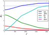 |
Fig. C.1. Power spectrum response Rℓ and its different terms. The dashed line indicates the effective value taken in the analysis (see main text). |
The total angular response shows some scale dependence over the range of multipoles considered, ranging from Rℓ ∼ 4.2 on large scales to Rℓ ∼ 5.5 on small scales. In this article for simplicity we took a constant effective value Rℓ = 5 (dashed line in Fig. C.1). This has the advantage of allowing analytical calculations in Sect. 3.4, and we find in Sect. 4 that it reproduces adequately the S/N over all scales considered, and also reproduces the Fisher constraints on cosmological parameters, except deep in the SSC-dominated regime for the most affected parameters.
To go beyond this constant Rℓ approximation, we need the scale dependence of the response. The redshift dependence is also needed, if we want to work on redshifts other than the one studied in this article (0.9 < z < 1). To answer both of these problems, we have computed numerically the full response through Eqs. (C.1) and (C.5) on scales 50 < ℓ < 2000 on a wide range of redshift (0.1 < z < 2 in bins Δz = 0.1). We then fitted the responses in each redshift bin either with a constant model  or a linear model Rℓ = R0 + R1 × (ℓ/ℓ0) with ℓ0 = 1000. The values of the fitted parameters are given in Table C.1.
Fits to the redshift dependence of the response of the galaxy power spectrum.
Another numerical approach that we anticipate is to calibrate the response through dedicated simulations, similarly to the work of Barreira et al. (2018b).
Appendix D: Impact of binning
Indicating bins of multipoles by the b subscript, the binned angular power spectrum, Cb, is defined as
 (D.1)
(D.1)
where the summation is over multipoles within the bin b, Δb is the width of the bin, and Sbℓ is a reshaping operator usually chosen to flatten the Cℓ within bins of multipoles11. This reshaping operator is thus obtained assuming that within the bin b, the angular power spectrum is approximately given by  with Cb a constant over the bin, and Sbℓ a (usually theoretically) known function of ℓ12. Finally, the widths of the bins are usually chosen to be greater than the typical length in multipoles of the ℓ-to-ℓ′ coupling induced by the mask.
The covariance of the binned spectrum, Cb, is related to the covariance of the full spectrum, Cℓ, as
 (D.2)
(D.2)
By writing Cov(Cℓ,Cℓ′) = 𝒞G + 𝒞SSC, the covariance of the binned spectra is then given by the sum of its Gaussian contribution and its super-sample contribution.
Choosing bins that are wider than the typical width of the mask-induced couplings leads to a diagonal Gaussian covariance (𝒞G)b, b′ ≃ Gbδb, b′. An analytic expression for Gb can be obtained assuming the fsky approximation, i.e.,
 (D.3)
(D.3)
Since the reshaping function is chosen such that SbℓCℓ is roughly constant, we can simplify the above to get  by defining the average multipole in the bin ℓb with the identification
  .
.
For the SSC, we first recall that for a single probe and a single redshift bin, the covariance of the spectra is given by
![Mathematical equation: $$ \begin{aligned} \left[\mathcal{C} _{\mathrm{SSC} }\right]_{\ell ,\ell ^{\prime }}=S_{i,i}V_\ell V_{\ell ^{\prime }}, \end{aligned} $$](/articles/aa/full_html/2019/04/aa34343-18/aa34343-18-eq134.gif) (D.4)
(D.4)
with Vℓ = RℓCℓ. It is then straightforward to show that for the binned spectra, we obtain
![Mathematical equation: $$ \begin{aligned} \left[\mathcal{C} _{\mathrm{SSC} }\right]_{b,b^{\prime }}=S_{i,i}V_b V_{b^{\prime }}, \end{aligned} $$](/articles/aa/full_html/2019/04/aa34343-18/aa34343-18-eq135.gif) (D.5)
(D.5)
with the binned version of the vector Vℓ, i.e.,
 (D.6)
(D.6)
In the case where the response Rℓ ≡ R is constant, this simplifies to Vb = RCb. This shows that for a single probe and a single bin in redshift, adding the SSC to covariance of binned power spectra still corresponds to a rank 1 update of the Gaussian covariance.
The above is easily generalized to the other cases where it is enlarged to multi-probes and more than one redshift bin since it is exactly the same binning in multipoles which has to be used for the entire set of multi-probe and multi-redshift auto- and cross-spectra. The data vector is now built from the multi-probe binned angular power spectra, and the vector Vb in the SSC is obtained by binning the vector Vℓ. Only the Gaussian covariance is slightly amended, being partitioned into nb × nb non-diagonal blocks of size nc × nc (nb is the number of bins and nc the number of auto- and cross-spectra). Using the fsky approximation, it becomes block diagonal 𝒞G = Gbδb, b′. The blocks of size nc × nc read
![Mathematical equation: $$ \begin{aligned} \left[{\boldsymbol{G}}_b\right]^{W,X;YZ}&\equiv {\mathrm{Cov} }_{\mathrm{G} }\left(C^{WX}_b,C^{YZ}_b\right) \nonumber \\&= \displaystyle \sum _{\ell \in b}\left(\frac{S_{b\ell }}{\Delta _b}\right)^2\times \left(\frac{ C^{WY}_\ell C^{XZ}_\ell +C^{WZ}_\ell C^{XY}_\ell }{(2\ell +1)\,f_{\mathrm{sky} } }\right), \end{aligned} $$](/articles/aa/full_html/2019/04/aa34343-18/aa34343-18-eq137.gif) (D.7)
(D.7)
where (W, X, Y, Z) run over probes.
Appendix E: Likelihood of cluster counts
The purpose of this section is to recall the form of the full likelihood of cluster counts, a result which seems overlooked in the literature. Further, we extend the likelihood with the formulation developed in Sect. 5.2, which will ensure it to be well-defined analytically.
We call N = (NiM, iz)iM, iz the vector of cluster counts in all bins of mass (indexed by iM) and redshift (indexed by iz). Then without super-sample covariance (simply called sample variance in the cluster literature), the likelihood is a collection of independent Poisson distribution in each bin of mass and redshift,
 (E.1)
(E.1)
where  is the model prediction for parameters p.
The above likelihood is sufficient to describe small counts, i.e., at high mass. However for current and future surveys detecting an increasing number of clusters, it becomes necessary to account for the effect of sample variance (Hu & Kravtsov 2003). Lima & Hu (2004) found the full likelihood for cluster counts in different cells, which can be straightforwardly applied to our case with only one cell (the survey),
 (E.2)
(E.2)
where S′ is similar to the S matrix defined in Eq. (5) in the case of cluster counts, but also including the counts response, and was defined originally for a 3D survey neglecting redshift evolution (Lima & Hu 2004):
 (E.3)
(E.3)
The matrix Siz; jz reads
 (E.4)
(E.4)
where  is the normalized (
 ) window function in redshift bin iz.
In the framework developed in Sect. 5.2,  is interpreted as the average number counts in a region of the universe having a background change δb. Noting that the response of the cluster counts is
  , we can rewrite the likelihood as
 (E.5)
(E.5)
 (E.6)
(E.6)
Rigorously, we might be concerned about the edges of the integral in this likelihood: it does not make physical sense for δb to go to −∞, as it corresponds to δN → −∞, i.e.,  becoming negative, which is impossible for a number of objects. In practice, this is unlikely to be a concern since for any reasonably sized survey the background change follows δb ≪ 1 at all redshifts, hence
  .
.
For the purpose of rigorousness, let us solve this physical concern nonetheless. When δb becomes of order 1, two approximations fail: (i) the pdf of δb being Gaussian, which is incorrect since for instance δb ≥ −1, and (ii) using a linear response ansatz  . Both failures can be cured formally with
 (E.7)
(E.7)
where P(δb|p) is the pdf of the background change (which has support on δb ∈ [−1, ∞[) and  is the average cluster count in a region with background change δb of a universe with cosmological parameters p. For instance in the separate universe approach this
  could be computed thanks to a change of cosmological parameters p′(p, δb).
All Tables
All Figures
|
Fig. 1. Comparison of the cumulative S/N values up to a multipole ℓmax with different covariances: Gaussian only, with the Si, j approximation, and with a full SSC computation. |
| In the text | |
|
Fig. 2. cos2θ for each cosmological parameter as a function of the maximum multipole ℓmax. Parameters with cos2θ close to 1 are the most affected by SSC when it starts to dominate the covariance (i.e., for multipoles ℓ ≳ ℓSSC with ℓSSC 360 in this specific case). |
| In the text | |
|
Fig. 3. Comparison of |
| In the text | |
|
Fig. C.1. Power spectrum response Rℓ and its different terms. The dashed line indicates the effective value taken in the analysis (see main text). |
| In the text | |
Current usage metrics show cumulative count of Article Views (full-text article views including HTML views, PDF and ePub downloads, according to the available data) and Abstracts Views on Vision4Press platform.
Data correspond to usage on the plateform after 2015. The current usage metrics is available 48-96 hours after online publication and is updated daily on week days.
Initial download of the metrics may take a while.