| Issue |
A&A
Volume 623, March 2019
|
|
|---|---|---|
| Article Number | L4 | |
| Number of page(s) | 6 | |
| Section | Letters to the Editor | |
| DOI | https://doi.org/10.1051/0004-6361/201834645 | |
| Published online | 01 March 2019 | |
Letter to the Editor
Topological model of the anemone microflares in the solar chromosphere
1
Sternberg Astronomical Institute (GAISh) of Lomonosov Moscow State University, Universitetskii prosp. 13, 119234 Moscow, Russia
e-mail: dumin@sai.msu.ru, dumin@yahoo.com
2
Space Research Institute (IKI) of Russian Academy of Sciences, Profsoyuznaya str. 84/32, 117997 Moscow, Russia
e-mail: somov@sai.msu.ru
Received:
14
November
2018
Accepted:
14
February
2019
Context. The chromospheric anemone microflares, which were discovered by Hinode satellite about a decade ago, are specific transient phenomena starting from a few luminous ribbons on the chromospheric surface and followed by an eruption upward. While the eruptive stage was studied in sufficient detail, a quantitative theory of formation of the initial multi-ribbon structure remains undeveloped until now.
Aims. We construct a sufficiently simple but general model of the magnetic field sources that is able to reproduce all the observed types of luminous ribbons by varying only a single parameter.
Methods. As a working tool, we employed the Gorbachev–Kel’ner–Somov–Shvarts (GKSS) model of the magnetic field, which was originally suggested about three decades ago to explain fast ignition of the magnetic reconnection over considerable spatial scales by tiny displacements of the magnetic sources. Quite unexpectedly, this model turns out to be efficient for the description of generic multi-ribbon structures in the anemone flares as well.
Results. As follows from our numerical simulation, displacement of a single magnetic source (sunspot) with respect to three other sources results in a complex transformation from three to four ribbons and then again to three ribbons, but with an absolutely different arrangement. Such structures closely resemble the observed patterns of emission in the anemone microflares.
Key words: magnetic fields / Sun: flares / Sun: magnetic fields
© ESO 2019
1. Introduction
One of the most interesting findings by the Hinode satellite (Kosugi et al. 2007; Tsuneta et al. 2008), which was obtained soon after beginning of its operation in 2006–2007, were the so-called anemone microflares observed in the chromospheric Ca II line (Shibata et al. 2007). Their development begins with three (or, less frequently, four) diverging ribbons in the horizontal plane and then, at the second stage, the entire structure erupts upward. Because of their similarity with sea anemones, such phenomena were called the anemone microflares1.
While the eruptive stage was studied in sufficient detail in a number of subsequent publications (Nishizuka et al. 2011; Singh et al. 2011, 2012), much less attention was paid to the formation of the initial multi-ribbon geometry. In fact, it was interpreted until now only in terms of the qualitative pictures of splitting magnetic tubes, such as in Fig. 3D,E by Shibata et al. (2007). In principle, it is not so difficult to invent some configuration of the magnetic sources that produces the required splitting of the magnetic fluxes. However, an interesting question arises: Is it possible to suggest a sufficiently simple but universal magnetic field model (e.g., involving a single free parameter) that would be able to describe all the observed types of anemone microflares?
Analysis of the various options that we performed recently has shown that a reasonable choice might be based on the model by Gorbachev et al. (1988), which we refer to as GKSS. This model was originally suggested as a mechanism for quick initiation of the magnetic reconnection in a considerable volume of space under a very small displacement of the magnetic sources, which was called the “topological trigger” of solar flares2. Surprisingly, it turns out that the same model can also serve for yet another purpose, i.e., the description of the multi-ribbon structures in the anemone microflares.
2. Theoretical model
The GKSS model of magnetic fields was originally derived by exploiting the quite sophisticated methods of differential geometry and algebraic topology, whose description is far beyond the scope of the present Letter; for mathematical details, see the above-mentioned paper by Gorbachev et al. (1988) and the later discussion by Brown & Priest (1999) and Somov (2013, Sect. 4.2). However, for the sake of completeness, we shall briefly summarize some basic facts.
Let us consider the four point-like magnetic sources (idealized sunspots) with equal magnitudes and opposite polarities (two positive and two negative) in the plane z = 0. Three of these are localized in the vertices of an equilateral rectangular triangle3, as shown in Fig. 1, while the fourth source can take different positions along the line y = 0.5.
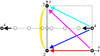 |
Fig. 1. Arrangement of the positive and negative magnetic sources and the corresponding semilunar region of topological instability (yellow) in the GKSS model. Four color arrows (red, magenta, blue, and cyan) designate four different types of topological connectivity of the magnetic field lines between these sources. Various positions of the fourth magnetic source, x4 = 1, 0.7, 0.4, 0.1, 0.0, −0.1, −0.4, −0.7, and −1.0, employed later, are shown by the black dotted circles. |
In the potential approximation4, the magnetic field formed by the above-mentioned sources can be evidently written as
where ei are the magnitudes of the sources and ri are their positions. In this work, e1 = e4 = 1 and e2 = e3 = −1.
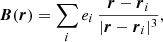
In general, the magnetic field in the entire half-space above the plane of sources is given by the so-called “two-dome configuration”. Namely, four spatial subregions resulting from the two intersecting domes (separatrices) correspond to the four types of connectivity of the magnetic field lines, connecting the positive and negative sources. As an example, Fig. 2 shows a base of the two-dome structure (i.e., its cross-section by the plane z = 0). The separatrices intersect each other in 3D space along the arc called the separator, which originates from the null points in z = 0 plane.
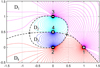 |
Fig. 2. Base of the two-dome structure at z = 0 (i.e., the “two-oval structure” drawn with dashed lines) for the particular arrangement of the fourth source, x4 = 0. Magnetic field lines with different connectivity are shown in red, magenta, blue, and cyan; these colors correspond to those in Fig. 1. The first (small) oval is separated in the domains D2 and D3 by the large oval. The domains D1 and D4 are outside the small oval and separated by the large oval, where D1 is the outer region. Small circles at the intersection of the oval boundaries are the null points of the magnetic field, which are the footpoints of the separator. |
Therefore, the magnetic field lines connecting the fourth and second sources fill the intersection of two domes, D3; and the lines connecting the fourth and third sources fill the small dome with the excluded intersection region, D2. The lines connecting the first and second sources are within the region D4, located in the large dome and outside the small dome. Finally, the lines connecting the first and third sources are within the outer space D1.
As was found by Gorbachev et al. (1988), when the fourth source is located in the crescent region of “topological instability” (shown in yellow in Fig. 1), the entire two-dome structure experiences a complex transformation (a kind of flip), resulting in the appearance of the additional (bifurcated) null point at the separator well above the plane of sources; and its position considerably changes under a tiny displacement of the fourth source (for recent observational evidence of this effect, resulting in the fast ignition of magnetic reconnection, see Dumin & Somov 2017).
Yet another interesting phenomenon, immediately related to the interpretation of anemone structures, can be found if we assume the existence of an energy-release region at the top of the separator. So, the energetic particles propagate downward along the magnetic field lines and, losing their energy, produce the emission spots at some height h; see Fig. 3. This is actually the same idea that was used a long time ago by Gorbachev & Somov (1988) for the interpretation of a two-ribbon structure in large solar flares. However, when the magnetic sources are arranged in the GKSS configuration, the pattern of splitting of their fluxes and the respective emission spots should be much more complex in the vicinity of the topologically unstable region. Therefore, we can expect the appearance of multi-ribbon structures. As shown in the next section, this hypothesis is well confirmed by rigorous numerical calculations.
 |
Fig. 3. Sketch of projections of the energy-release regions with various radii R (indicated by red, magenta, green, blue, and cyan) along the magnetic field lines onto the plane located at height h above the field sources. The sources are denoted by asterisks and the vertical projection of the center of the energy-release region is denoted by a small thick circle. |
3. Results of calculations
The basic domain of computation is presented in Fig. 3: The point-like magnetic sources with coordinates (x1, y1), (x2, y2), (x3, y3), and (x4, y4) are located in the plane z = 0; these sources can be physically interpreted as sunspots in the solar photosphere. The separator, where two “magnetic domes” (separatrices) intersect each other, has footpoints (xf1, yf1) and (xf2, yf2) in the same plane, and its vertex is in the point (xv, yv, zv) above this plane. Their numerical values at various positions of the fourth source x4 are listed in Table A.1; the algorithm employed for their computation is outlined in Appendix A. In addition, all these characteristic points of the separator as functions of x4 are pictorially represented in Fig. 4.
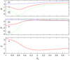 |
Fig. 4. Coordinates x, y, and z (top, middle, and bottom panels, respectively) of the first footpoint (dashed blue curves, denoted by “f1”), second footpoint (dotted green curves, denoted by “f2”), and vertex of the separator (solid red curve, denoted by “v”) as functions of the position of the fourth magnetic source x4. |
Then, we consider a set of the energy-release regions in the form of balls with various radii R, whose centers are in the vertex of the separator (xv, yv, zv); they are indicated by different colors in Fig. 3. Next, we take the initial points uniformly distributed over the surface of the corresponding ball (with mutual separation, for example, 15°) and integrate the standard equations for the magnetic field lines,
either in forward or backward direction (i.e., increasing or decreasing l) until they intersect the plane located below at height h. From the physical point of view, this means that charged particles are accelerated in the energy-release region, propagate along the field lines, and finally are decelerated and lose their energy in the denser layer of the solar atmosphere at z = h. Hence, the corresponding plane is called the plane of emission. Projections of the energy-release regions onto this plane are shown by the dotted areas of the respective colors. They have a granular structure in Fig. 3 only because we traced a finite number of magnetic field lines.
The numerical calculations of the above-mentioned projections were performed for different positions of the fourth magnetic source x ∈ [ − 1, 1] along the line y = 0.5. Along with that, we studied how the pattern of projections depend on the parameters R and h. A particular example for x4 = 1.0, 0.7, 0.4, 0.1, 0.0, −0.1, −0.4, −0.7, −1.0,R = 0.05, 0.10, 0.15, 0.25, 0.35, and h = 0.3 (everything in dimensionless units, normalized to the separation between the magnetic sources) is presented in Fig. 5.
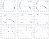 |
Fig. 5. Calculated projections of the energy-release region (taken at the top of the separator) along the magnetic field lines onto the horizontal plane (located at the height h = 0.3 above the plane of magnetic sources) at various positions of the fourth source x4. The red, magenta, green, blue, and cyan points correspond to the various radii of the energy-release region R = 0.05, 0.10, 0.15, 0.25, and 0.35, respectively. Positions of the magnetic field sources are denoted by the asterisks, and vertical projections of the energy-release regions are shown by the small circles. |
4. Discussion and conclusions
As is seen in Fig. 5, the spots of emission in the h-plane (which can be interpreted as chromosphere, located above the photospheric sources) experience a drastic transformation when the fourth magnetic source shifts to the left, as depicted in Fig. 1:
-
Initially, at x4 = 1.0, 0.7, and 0.4, the situation resembles the classical two-ribbon flare, as was found earlier by Gorbachev & Somov (1988).
-
Next, near the region of topological instability (x4 = 0.1 and 0.0), these ribbons become distorted and subdivided into three parts.
-
Then, immediately in the region of topological instability (x4 = −0.1), we get a four-ribbon structure.
-
At last, when the fourth source moves further to the left (x4 = −0.4, −0.7, and −1.0), the four ribbons merge again into three ribbons, but with an absolutely different spatial arrangement.
The above-listed configurations closely resemble chromospheric anemone flares, possessing usually three and, less frequently, four ribbons, as seen in the numerous movies available in the Hinode archive5. To avoid misunderstanding, let us emphasize that various values of x4 correspond to a statistical sample of various microflares. They should not be interpreted as a real physical motion of the fourth source in the course of the flare development, since the lifetime of such flares is very short.
As regards the dependence of the emission ribbons on the radii R, we can see a quite complicated behavior. In the two- and four-ribbon configurations, a core of the energy-release region (i.e., the balls with smaller R) is projected into the centers of the ribbons and the outer part (with larger R) into their periphery (see panels with x4 = 1.0, 0.7, 0.4, and −0.1 in Fig. 5). However, in the three-ribbon configurations, both on the right- and left-hand side of the topological instability region, the situation is different. One ribbon looks as described above while in two other ribbons the inner and outer parts of the energy-release region tend to project into the opposite sides of the strips (see panels with x4 = 0.1, −0.7, and −1.0).
At last, as follows from our computations of the emission ribbons at various heights h (not represented in detail in this Letter), the corresponding patterns remain qualitatively the same such that only the degree of expression of the ribbons (i.e., the sharpness and separation between them) varies. In fact, the best expression takes place just at the height about h = 0.3, which is presented in Fig. 5.
In principle, it might also be interesting to study the dependence of the emission spots on the position of the energy-release region along the separator. However, in this paper we studied only the case of very small magnetic loops, corresponding to the microflares. In fact, a height of the arc was only two to three times greater than the height of the plane of emission above the plane of sources, and the size of the energy-release region was of the same order of magnitude. Therefore, in these conditions, it was impossible to analyze any substantial shifts of the energy-release region along the separator. Nevertheless, some hints concerning this issue can be drawn from the behavior of the emission spots as function of the radii of the energy-release spheres R, which are plotted by various colors in Figs. 3 and 5.
We also checked the patterns of emission obtained under the similar assumptions in a few other topological models of solar magnetic fields (i.e., involving the bifurcations of null points). In these models, however, we did not find the behavior of the ribbons as rich as in the GKSS model. This is most probably because only the latter model exhibits the genuine topological instability, i.e., when a small rearrangement of the magnetic sources results in the dramatic reconstruction of the magnetic field lines in the entire space.
In summary, the four-ribbon configurations exist only in a quite small semilunar region of topological instability (where the bifurcation takes place); at all other locations of the fourth magnetic source, a three- (or even two-)ribbon emission appears. Hence, we should expect that fraction of the four-ribbon flares will be sufficiently small because of the relatively small area of the region of topological instability. This prediction agrees very well with the observations. Most of the anemone flares detected by Hinode satellite possess three ribbons; the four-ribbon flares also exist but they are formed seldomly. This is why we believe that our topological model, although not universal, provides a reasonable interpretation of the relevant phenomena by varying only a single parameter.
At the same time, the term “anemone” was used also to denote some types of active regions and the corresponding large solar flares (Asai et al. 2009), which are unrelated to the microflares discussed in the present paper.
Some more sophisticated topological models of the solar magnetic fields were suggested, for example, by Inverarity & Priest (1999) and Brown & Priest (2001); their review was given by Longcope (2005). The applications of topological methods to various solar phenomena were reviewed by Janvier (2017).
From the physical point of view, the potential approximation implies that the magnetic field in the volume under consideration is produced mostly by the sources at its boundaries, while contribution by the bulk electric currents is negligible. Effects of the electric currents on global topology of the magnetic field lines were analyzed, e.g., by Brown & Priest (2000).
Acknowledgments
YVD is grateful to P.M. Akhmet’ev and E.V. Zhuzhoma for consultations on the topological issues, as well as to A.V. Getling, A.V. Oreshina, and I.V. Oreshina for help in processing the data on magnetic fields. BVS was supported by the Russian Foundation for Basic Research, grant no. 16-02-00585.
References
- Asai, A., Shibata, K., & Ishii, T. T. 2009, J. Geophys. Res., 114, A00A21 [Google Scholar]
- Brown, D. S., & Priest, E. R. 1999, Sol. Phys., 190, 25 [NASA ADS] [CrossRef] [Google Scholar]
- Brown, D. S., & Priest, E. R. 2000, Sol. Phys., 194, 197 [NASA ADS] [CrossRef] [Google Scholar]
- Brown, D. S., & Priest, E. R. 2001, A&A, 367, 339 [NASA ADS] [CrossRef] [EDP Sciences] [Google Scholar]
- Dumin, Y. V., & Somov, B. V. 2017, Res. Notes Amer. Astron. Soc., 1, 15 [NASA ADS] [CrossRef] [Google Scholar]
- Gorbachev, V. S., Kel’ner, S. R., Somov, B. V., & Shvarts, A. S. 1988, Sov. Astron., 32, 308 [NASA ADS] [Google Scholar]
- Gorbachev, V. S., & Somov, B. V. 1988, Sol. Phys., 117, 77 [NASA ADS] [CrossRef] [Google Scholar]
- Inverarity, G. W., & Priest, E. R. 1999, Sol. Phys., 186, 99 [NASA ADS] [CrossRef] [Google Scholar]
- Janvier, M. 2017, J. Plas. Phys., 83, 535830101 [Google Scholar]
- Kosugi, T., Matsuzaki, K., Sakao, T., et al. 2007, Sol. Phys., 243, 3 [NASA ADS] [CrossRef] [Google Scholar]
- Longcope, D. W. 2005, Liv. Rev. Sol. Phys., 2, 7 [Google Scholar]
- Nishizuka, N., Nakamura, T., Kawate, T., Singh, K. A. P., & Shibata, K. 2011, ApJ, 731, 43 [NASA ADS] [CrossRef] [Google Scholar]
- Shibata, K., Nakamura, T., Matsumoto, T., et al. 2007, Science, 318, 1591 [NASA ADS] [CrossRef] [Google Scholar]
- Singh, K. A. P., Shibata, K., Nishizuka, N., & Isobe, H. 2011, Phys. Plas., 18, 111210 [Google Scholar]
- Singh, K. A. P., Isobe, H., Nishizuka, N., Nishida, K., & Shibata, K. 2012, ApJ, 759, 33 [NASA ADS] [CrossRef] [Google Scholar]
- Somov, B. V. 2013, Plasma Astrophysics, Part II: Reconnection and Flares, 2nd edn. (New York: Springer) [CrossRef] [Google Scholar]
- Tsuneta, S., Suematsu, Y., Ichimoto, K., et al. 2008, Sol. Phys., 249, 167 [NASA ADS] [CrossRef] [Google Scholar]
Appendix A: Basic parameters of the separator in the two-dome structure
In general, computing a spatial configuration of the separator is a non-trivial task: the separator is an inherently unstable structure, since any field line originating in its neighborhood quickly deviates outward. So, the straightforward numerical integration is meaningless, and a more elaborate type of algorithm should be applied. In the present work, we used the following procedure:
-
Since footpoints of the separator, (xf1, yf1) and (xf2, yf2), are actually the null points of the magnetic field in z = 0 plane, we calculated the distribution of B2 in this plane, sought for its minima, and finally checked that B2 = 0 in these minima (and, therefore, B = 0). The analysis of the scalar function B2(x, y) was employed only because, from the computational point of view, it is much more simple and robust than the analysis of the vector field B(x, y).
-
To find a position of the separator above the plane z = 0, we analyzed the following “global” behavior of the magnetic field lines:
(a) First of all, we fixed a vertical plane intersecting the line connecting the opposite footpoints of the separator (xf1, yf1, 0) and (xf2, yf2, 0); to get a better accuracy, it is desirable that this plane be approximately perpendicular to the line.
(b) Then, we generated a mesh of points in the above-mentioned plane; and each of these points was used as the initial condition for integration of the magnetic field line Eq. (2) in the forward and backward directions until the corresponding field line entered one of the magnetic sources e1, e2, e3, or e4. Thereby, the sketch of topological connectivity, composed of four subregions whose field lines terminate at four different sources, is obtained. These subregions touch each other in some spot, which is just the place where separator intersects the specified plane.
(c) Next, we fixed a smaller rectangle covering the above-mentioned spot, generated a finer mesh of initial points, and performed the same procedure as in the previous item.
(d) Repeating these steps a few times, we can localize the spot of intersection of the separator with the specified plane as accurately as desired.
(e) If necessary, the points of intersection with a set of planes can be interpolated between each other to get the intermediate positions of the separator.
The most important parameters of the resulting separators–the coordinates of their footpoints and vertices–at various positions of the fourth source (x4, 0.5) are listed in Table A.1 and drawn in Fig. 4.
Computed coordinates of the separator’s footpoints (xf1, yf1, 0) and (xf2, yf2, 0) and of its vertex (xv, yv, zv), where the energy-release region is located, at various positions x4 of the fourth magnetic field source.
All Tables
Computed coordinates of the separator’s footpoints (xf1, yf1, 0) and (xf2, yf2, 0) and of its vertex (xv, yv, zv), where the energy-release region is located, at various positions x4 of the fourth magnetic field source.
All Figures
|
Fig. 1. Arrangement of the positive and negative magnetic sources and the corresponding semilunar region of topological instability (yellow) in the GKSS model. Four color arrows (red, magenta, blue, and cyan) designate four different types of topological connectivity of the magnetic field lines between these sources. Various positions of the fourth magnetic source, x4 = 1, 0.7, 0.4, 0.1, 0.0, −0.1, −0.4, −0.7, and −1.0, employed later, are shown by the black dotted circles. |
| In the text | |
|
Fig. 2. Base of the two-dome structure at z = 0 (i.e., the “two-oval structure” drawn with dashed lines) for the particular arrangement of the fourth source, x4 = 0. Magnetic field lines with different connectivity are shown in red, magenta, blue, and cyan; these colors correspond to those in Fig. 1. The first (small) oval is separated in the domains D2 and D3 by the large oval. The domains D1 and D4 are outside the small oval and separated by the large oval, where D1 is the outer region. Small circles at the intersection of the oval boundaries are the null points of the magnetic field, which are the footpoints of the separator. |
| In the text | |
|
Fig. 3. Sketch of projections of the energy-release regions with various radii R (indicated by red, magenta, green, blue, and cyan) along the magnetic field lines onto the plane located at height h above the field sources. The sources are denoted by asterisks and the vertical projection of the center of the energy-release region is denoted by a small thick circle. |
| In the text | |
|
Fig. 4. Coordinates x, y, and z (top, middle, and bottom panels, respectively) of the first footpoint (dashed blue curves, denoted by “f1”), second footpoint (dotted green curves, denoted by “f2”), and vertex of the separator (solid red curve, denoted by “v”) as functions of the position of the fourth magnetic source x4. |
| In the text | |
|
Fig. 5. Calculated projections of the energy-release region (taken at the top of the separator) along the magnetic field lines onto the horizontal plane (located at the height h = 0.3 above the plane of magnetic sources) at various positions of the fourth source x4. The red, magenta, green, blue, and cyan points correspond to the various radii of the energy-release region R = 0.05, 0.10, 0.15, 0.25, and 0.35, respectively. Positions of the magnetic field sources are denoted by the asterisks, and vertical projections of the energy-release regions are shown by the small circles. |
| In the text | |
Current usage metrics show cumulative count of Article Views (full-text article views including HTML views, PDF and ePub downloads, according to the available data) and Abstracts Views on Vision4Press platform.
Data correspond to usage on the plateform after 2015. The current usage metrics is available 48-96 hours after online publication and is updated daily on week days.
Initial download of the metrics may take a while.