| Issue |
A&A
Volume 623, March 2019
|
|
|---|---|---|
| Article Number | A100 | |
| Number of page(s) | 8 | |
| Section | Planets and planetary systems | |
| DOI | https://doi.org/10.1051/0004-6361/201834577 | |
| Published online | 08 March 2019 | |
A Jovian planet in an eccentric 11.5 day orbit around HD 1397 discovered by TESS
1
Geneva Observatory, University of Geneva,
Chemin des Mailettes 51,
1290
Versoix,
Switzerland
e-mail: This email address is being protected from spambots. You need JavaScript enabled to view it.
2
Institute for Computational Science, University of Zurich,
Winterthurerstrasse 190,
8057
Zurich,
Switzerland
3
Department of Earth Sciences, University of California,
Riverside,
CA
92521,
USA
4
University of Southern Queensland,
Centre for Astrophysics,
Toowoomba,
QLD 4530,
Australia
5
SETI Institute,
Mountain View,
CA
94043,
USA
6
Proto-Logic LLC,
Washington,
DC
20009,
USA
7
Harvard-Smithsonian Center for Astrophysics,
60 Garden Street,
Cambridge,
MA
02138,
USA
8
Department of Physics and Kavli Institute for Astrophysics and Space Research, MIT,
Cambridge,
MA
02139,
USA
9
Department of Physics, Lehigh University,
16 Memorial Drive East,
Bethlehem,
PA
18015,
USA
10
Leidos/NASA Ames Research Center,
Moffett Field,
CA
94035,
USA
11
Department of Physics & Astronomy, Vanderbilt University,
6301 Stevenson Center Ln.,
Nashville,
TN
37235,
USA
12
Department of Earth, Atmospheric, and Planetary Sciences, and Department of Aeronautics and Astronautics, MIT,
77 Massachusetts Avenue,
Cambridge,
MA
02139,
USA
13
Department of Astrophysical Sciences, Princeton University,
4 Ivy Lane,
Princeton,
NJ
08544,
USA
14
NASA Ames Research Center,
Moffett Field,
CA
94035,
USA
15
Caltech/IPAC-NASA Exoplanet Science Institute,
M/S 100-22, 770 S. Wilson Ave,
Pasadena,
CA
91106,
USA
16
UC Santa Cruz, Department of Astronomy & Astrophysics,
1156 High Street,
Santa Cruz,
CA
95064,
USA
17
NASA Goddard Space Flight Center,
8800 Greenbelt Rd.,
Greenbelt,
MD
20771,
USA
18
Department of Astronomy, The University of Texas at Austin,
2515 Speedway C1400,
Austin,
TX
78712,
USA
19
Department of Physics and Astronomy, University of Louisville,
Louisville,
KY
40292,
USA
20
Astronomy Department, University of Florida,
211 Bryant Space Science Center, PO Box 112055,
Gainesville,
FL
32611-2055,
USA
21
Department of Physics and Astronomy, George Mason University,
Fairfax,
VA
22030,
USA
22
Exoplanetary Science at UNSW, School of Physics,
UNSW Sydney,
NSW 2052,
Australia
23
School of Astronomy and Space Science, Key Laboratory of Ministry of Education, Nanjing University,
Nanjing,
PR China
Received:
5
November
2018
Accepted:
18
February
2019
Abstract
The Transiting Exoplanet Survey Satellite TESS has begun a new age of exoplanet discoveries around bright host stars. We present the discovery of HD 1397b (TOI-120.01), a giant planet in an 11.54-day eccentric orbit around a bright (V = 7.9) G-type subgiant. We estimate both host star and planetary parameters consistently using EXOFASTv2 based on TESS time-series photometry of transits and radial velocity measurements with CORALIE and MINERVA-Australis. We also present high angular resolution imaging with NaCo to rule out any nearby eclipsing binaries. We find that HD 1397b is a Jovian planet, with a mass of 0.415 ± 0.020 MJ and a radius of 1.026 ± 0.026 RJ. Characterising giant planets in short-period eccentric orbits, such as HD 1397b, is important for understanding and testing theories for the formation and migration of giant planets as well as planet-star interactions.
Key words: planets and satellites: detection / planets and satellites: individual: HD 1397b / planets and satellites: individual: TOI-120 / planets and satellites: individual: 394137592
© ESO 2019
1 Introduction
Transiting exoplanets offer a unique window into exoplanetology, because we can measure both the mass and radius of the planet, and thereby place constraints on the interior structure. Atmospheric characterisation is also possible through transmission spectroscopy, thus enabling a full understanding of bulk properties and atmosphere.
After the recent end of the NASA Kepler and K2 missions, the exoplanet-finding torch has truly been passed on to the Transiting Exoplanet Survey Satellite (TESS; Ricker et al. 2015). Since the start of science operations on July 25, 2018, TESS has successfully delivered several hundred exoplanet candidates, and the first few planet confirmations have been reported e.g. Huang et al. (2018), Gandolfi et al. (2018), Vanderspek et al. (2019), and Wang et al. (2019).
In this paper we present the discovery of a jovian planet in an eccentric 11.54-day orbit around HD 1397, a bright (V = 7.9) sub-giant star from TESS with a mass characterisation enabled by CORALIE and MINERVA-Australis.
2 Observations
2.1 TESS photometry
HD 1397b (TIC 394137592) was observed by TESS between 2018 Jul 25 and Sep 20, in the first of the 26 sectors of the two-year survey. The target appeared on Camera 3, CCD 1 in TESS sector 1, and was observed with both 2 min cadence data and the 30 min cadence Full Frame Images. We used the publicly available TESS sector 1 data with 2-min cadence, supplied through the TESS Alert mechanism. They were reduced with the Science Processing Operations Center (SPOC) pipeline, originally developed for the Kepler mission at the NASA Ames Research Center (Jenkins 2017; Jenkins et al. 2016). Two transits of HD 1397b were detected with signal-to-noise ratio (S/N) of 81.0 (Jenkins 2002; Jenkins et al. 2017; Twicken et al. 2018). For transit modelling, we used the raw light curve based on the Pre-search Data Conditioning data product (Twicken et al. 2010; see Sect. 3.3). The light curve precision is 144 ppm, averaged over one hour, consistent with the value predicted by Sullivan et al. (2015).
2.2 High resolution spectroscopy with CORALIE
HD 1397 was observed with the high resolution spectrograph CORALIE on the Swiss 1.2 m Euler telescope at La Silla Observatory (Queloz et al. 2001a) between 2018 Sep 8 and 2018 Dec 20. CORALIE is fed by a 2′′ fibre and has resolution R = 60 000. In total 42 measurements were obtained. For three of them the simultaneous drift computation failed due to abnormal instrument drift, and thus these three observations are left out of the radial velocity (RV) analysis, but included in the spectral analysis.
Radial velocities and line bisector spans were calculated via cross-correlation with a G2 binary mask, using the standard CORALIE data-reduction pipeline. Given the bright magnitude of HD 1397, we are not limited by photon noise, but rather the instrumental noise floor for CORALIE at around 3 m s−1. The first few measurements were used for reconnaissance, to check for a visual or spectroscopic binary. Once we saw that the 35 m s−1 difference inRV was consistent with the ephemerides provided by TESS we commenced intensive follow-up observations covering more than 3 orbits. For one orbit, we aimed at obtaining two RV points per night to check for any shorter-period planets. The RVs, along with associated properties, are given in Table 1. In Fig. 1, we plot the RV time series along with our result from the joint modelling analysis (see Sect. 3.3).
To ensure that the RV signal does not originate from cool stellar spots or a blended eclipsing binary, we checked for correlations between the line bisector span and the RV measurements (Queloz et al. 2001b). We find no evidence for a correlation. A full treatment of the line bisector and activity indicators can be found in Sect. 3.2. All the CORALIE spectra were combined in the stellar rest frame into one high signal-to-noise spectrum for spectral characterisation (see Sect. 3.1).
Radial velocities from CORALIE and MINERVA-Australis.
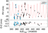 |
Fig. 1 Timeseries of the CORALIE and MINERVA-Australis RVs with the EXOFASTv2 two Keplerian model over-plotted in red. |
2.3 High resolution spectroscopy with MINERVA-Australis
HD 1397 was observed with the MINiature Exoplanet Radial Velocity Array (MINERVA-Australis) located in Queensland, Australia on 7 nights between 2018 Sep 9 and 2018 Oct 2. MINERVA-Australis (Addison et al. 2019) is an array of 0.7 m telescopes feeding a stabilised R = 80 000 spectrograph functionally identical to the US-based MINERVA array (Swift et al. 2015). At this writing, MINERVA-Australis hosts a single 0.7 m telescope (with a further four to be installed in 2019), feeding starlight via a 2.2′′ fibre into the spectrograph (Wright et al., in prep). Wavelength calibration is achieved by a simultaneous ThAr lamp calibration fibre, and radial velocities are obtained by an implementation of standard mean-spectrum least-squares matching procedures (Anglada-Escudé & Butler 2012). A total of 25 individual measurements were obtained; data from 16 Sep were excluded from the analysis due to extremely poor observing conditions.
2.4 High angular resolution imaging with VLT/NaCo
HD 1397 was observed with NaCo (Rousset et al. 2003; Lenzen et al. 2003) on the UT4 telescope of the Very Large Telescope at Paranal Observatory, on the night of 2018 Oct 24. A total of 54 exposures of 4 s each were collected using the narrowband Br-γ filter (λc = 2.166 μm). The target was centred within the upper left quadrant of the detector, and the telescope dithered by 2′′ after every second integration, with a sub-field of 4′′ centred on the target covered by all dithers. Images were dark subtracted and flat fielded, and the dithered images used to remove the sky background. The images were then aligned and median combined. No additional sources were identified anywhere within the final mosaiced image, which extends to at least 6 arcsec from the target in every direction. The target appears to be single, to the limit of the imaging resolution. To determine the sensitivity of the final combined images, simulated PSF images were inserted into the data and recovered with standard aperture photometry. A sensitivity curve is shown in Fig. 2 along with the high angular resolution image of the target.
3 Analysis and results
3.1 Stellar parameters through spectral analysis
The 42 CORALIE spectra were stacked in the stellar rest frame, weighted by the individual signal-to-noise ratio to create one high quality spectrum. Bulk stellar parameters were derived using SPECMATCH-EMP (Yee et al. 2017), which matches the input spectra to a vast library of stars with well-determined parameters derived with a variety of independent methods, e.g. interferometry, optical and NIR photometry, asteroseismology, and LTE analysis of high-resolution optical spectra. We used the spectral region around the Mgb triplet (5100–5340 Å) to match our spectrum to the library spectra through χ2 minimisation. A weighted linear combination of the five best matching spectra were used to extract Teff, log g and [Fe/H].
We adopted Teff, and [Fe/H] obtained for the stacked spectrum as priors for the global modelling. The final stellar bulk parameters, including mass and radius, are modelled jointly with the planetary parameters within EXOFASTv2 as described in Sect. 3.3. This method utilises the transit light curve, SED fitting of archival broad band photometry, and the Gaia parallax along with stellar tracks and isochrones. We obtain stellar radius of  R⊙ and mass
  M⊙, as summarised in Table 2.
The projected rotational velocity of the star, vsini, was computed using the calibration between vsini and the width of the CCF from Santos et al. (2002) for CORALIE. The formal result was smaller than what can be resolved by CORALIE, and we can therefore only establish an upper limit of 2 km s−1.
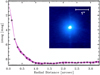 |
Fig. 2 Sensitivity curve from NaCo AO imaging at Br-γ. The inset image is 3 arcsec on either side. |
3.2 Stellar rotation and activity
To constrainthe rotation period and overall stellar variability of the star we computed the time series of several spectroscopic line indicators from the CORALIE spectra. We based our analysis on the Mount Wilson Ca II H&K S-index (Noyes et al. 1984; Lovis et al. 2011), the Hα index (Gomes da Silva et al. 2011), He I index (Boisse et al. 2009), NA I index (Díaz et al. 2007) and TiO index (Azizi & Mirtorabi 2018). We compute the power spectrum of the different time series using a generalised Lomb-Scargle periodogram (Zechmeister & Kürster 2009). We then fit a double sinusoidal model at the detected period, and the first harmonic of the period, whenever there is a significant signal, in the similar way as Suárez Mascareño et al. (2017), only this time adding a jitter parameter to the fit.
We found evidence of variability on timescales compatible with stellar rotation. The bisector span, FWHM of the CCF, Ca II H&K S-index, Hα index and He I index show detections of periodicities in the range of 40–50 days (see Fig. 3). We find no significant evidence of periodic variability in the Na I and TiO time series. This suggests the possibility of a rotation period of 42.5 ± 3.4 days, which would be reasonable for an evolved star, and would indicate an inclination of the rotation axis smaller than 46°, considering the small vsini. This measurement should be taken with caution, as the baseline of our observations only cover two rotational periods.
We find evidence that the stellar activity is affecting the RVs. When fitting a single 11.54 day Keplerian orbit to the CORALIE RVs, the residuals correlate moderately with the Hα index (r ~ 0.49). Detrending the RVs by subtracting a linear model between the two quantities does not affect the planetary detection, but reduces the planetary mass and orbital eccentricity slightly. This is taken into account in the joint modelling, as described in Sect. 3.3.
Stellar properties for HD 1397.
3.3 Jointmodelling with EXOFASTv2
Simultaneous and self-consistent fitting of the CORALIE and MINERVA-Australis radial velocities, TESS transit light curves and stellar parameters was performed using EXOFASTv2 (see Eastman 2017; Eastman et al. 2013, for a full description). This joint model enforces global consistency of the stellar and planetary properties with all of the available data. The parameter space is explored with a differential evolution Markov Chain method through 50 000 steps and 16 independent chains. EXOFASTv2 has build-in diagnostics for checking how well the chains are mixing through Gelman–Rubin statistic (Gelman et al. 2003) as proposed by Ford (2006). In our case the Gelman-Rubin statistic indicated that all fitted parameters were well mixed. In total 31 free parameters are fitted, for which four (log g, [Fe∕H], Prot and the parallax) have constraining Gaussian priors, described in this section.
The parameters logg and [Fe∕H] obtained from the spectroscopic analysis were used as Gaussian priors. Broadband photometry, the Gaia DR2 parallax and an upper limit on the V -band extinction from Schlegel et al. (1998) and Schlafly & Finkbeiner (2011) were also used as input, to model the stellarproperties consistently with the planet parameters through SED fitting. The Gaia DR2 parallax is a powerful parameter for computing stellar properties. For completeness, we adjusted the parallax by + 0.07 mas based on the systematic offsets reported by Stassun & Torres (2018) and by Zinn et al. (2018). Both studies find the Gaia DR2 parallaxes to be too small by 0.06–0.08 mas from benchmark eclipsing binary and asteroseismic stars within ~1 kpc. For HD 1397 the offset represents only ~0.5% error on the parallax. However, as our aim is to achieve a precision on the radius of a few percent or better, this 0.5% systematic error is not entirely negligible. Within EXOFASTv2 we invoked the Mesa Isochrones and Stellar Tracks (MIST, Dotter 2016; Choi et al. 2016) to model the star. We compared results using the Torres radius-mass relationship (Torres et al. 2010)and YY-isochrones (Yi et al. 2001), which showed no significant discrepancies in stellar, nor planetary, properties. The final SED fit is shown in Fig. 4.
As demonstrated in Sect. 3.2, HD 1397 is an active star which affects the RVs. To correct for the stellar activity we model the stellar rotation as an additional Keplerian with a Gaussian prior on the period from the analysis of the spectral indicators (Prot = 42.5 ± 3.4). A more ideal solution could be to detrend the RVs directly with an activity indicator, e.g. the Hα index, but this is currently not possible within EXOFASTv2. Further more, we only have derived activity indicators for the CORALIE data, and would thus have to interpolate those in order to detrend the MINERVA-Australis data. We have performed an independent analysis of the CORALIE data detrended against the Hα index, and obtained results for the planetary parameters which were consistent with the EXOFASTv2 global model with two Keplerians. When modelling two Keplerians in EXOFASTv2, we obtain a period of  days for the stellar activity cycle.
The joint analysis shows clear evidence of a 0.415 ± 0.020MJ and 1.026 ± 0.026RJ planet in an eccentric orbit (e = 0.251 ± 0.020). The adopted solution with two Keplerians is illustrated in Fig. 1 where the RV time series are plotted along with the best-fitting model.
The period of 11.5353 ± 0.0008 days is well constrained, even with only two TESS transits. A full summary of the results from the joint modelling can be seen in Tables 2 and 3, listing the stellar and planetary properties, respectively. The fit to the transit light curves can be seen in Fig. 5, where the two TESS transits have been phase-folded along with the final model from EXOFASTv2.
The host star is a slightly evolved G-type sub-giant with radius  R⊙ and mass
  M⊙. The age of the system is estimated to be 4.51 ± 0.5 Gyr which is consistent with the evolutionary stage of a star with this mass. HD 1397b has a mean density of
  g cm−3, making it a low-density exoplanet.
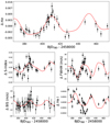 |
Fig. 3 Time series of the Hα index (top panel), Ca II H&K S-index (middle left panel), FWHM (middle right panel), bisector span (bottom left panel) and He I index (bottom right panel) for the CORALIE spectra. The red lines show the best fit to the data. |
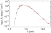 |
Fig. 4 SED fitting of HD 1397 as produced by EXOFASTv2. The sources of the broad band photometry is detailed in Table 2. |
4 Discussion and conclusion
We present the discovery of a hot Jupiter in an 11.54 day orbit with eccentricity of 0.251 ± 0.020, around a bright, V = 7.8, G-type sub-giant1. Planetary and stellar parameters were modelled jointly using both TESS transit light curves and CORALIE and MINERVA-Australis radial velocities to ensure consistent results. Through high angular resolution imaging we have also ruled out the possibility of nearby stellar companions. HD 1397b will, along with all the coming giant planets from TESS, help our understanding of giant planet formation, evolution and dynamics.
HD 1397b is unusual in that it is a close-in planet orbiting a somewhat evolved intermediate-mass star. Nearly two decades of RV surveys for planets orbiting such stars have yielded only a handful of planets with a < 0.5 au. The majority of those surveys have targeted subgiants or low-luminosity giants (e.g. Frink et al. 2001; Johnson et al. 2010; Jones et al. 2011; Wittenmyer et al. 2011), which have not yet expanded to engulf such planets (Kunitomo et al. 2011). Statistical analyses from these surveys have so far generally agreed that giant planets are rare within 0.5 au (Bowler et al. 2010), and that the overall occurrence rate of planets is positively correlated with both host-star mass and metallicity (Jones et al. 2014; Reffert et al. 2015; Wittenmyer et al. 2017a). Tidal effects for eccentric planets orbiting giant stars result in significant tidal decay of the orbits, resulting in predictions regarding when the planet may merge with the host star (Wittenmyer et al. 2017b). In the case of HD 1397b, the periastron passage of the planet bring it within ~8 stellar radii of the host star.
The source of HD 1397b’s eccentricity adds further interest to this system. It has been shown that sparse sampling and noisy RV data can cause circular double-planet systems to be misinterpreted as single eccentric planets (e.g. Wittenmyer et al. 2013; Trifonov et al. 2017; Boisvert et al. 2018). In this case however, the transit detection gives assurance that the RV variations are indeed due to a single planet on an eccentric orbit. There are numerous possible origins for the nonzero orbital eccentricity, including angular momentum transfer from an additional planet in the system (Kane & Raymond 2014), prior planet–planet scattering events (Ford & Rasio 2008), or the close passage of a stellar binary companion (Halbwachs et al. 2005; Kane et al. 2014). Examples of the latter scenario include the extreme eccentricity cases of HD 80606b (Liu et al. 2018), HD 4113b (Cheetham et al. 2018), and HD 20782b (Kane et al. 2016). At the present time, our data show no significant evidence for the presence of a second planet, nor is there observational evidence for a bound stellar companion to the host star.
Thus a likely scenario for the eccentricity of the orbit is perturbations from the star–planet system during the evolution of the star off the main sequence. For example, the study by Grunblatt et al. (2018) of eccentric planetary orbits associated with evolved stars concluded that the difference between tidal circularization time scales and the orbital evolution that occurs during host star mass loss may account for the observed eccentricity distribution around giant stars (Villaver & Livio 2009; Villaver et al. 2014; Veras 2016). For HD 1397b, as a well-characterised planet transiting a bright star, further RV measurements will either strengthen this explanation or possibly reveal evidence of additional bodies in this fascinating system.
Jovian planets around stars that are moving up the sub-giant and red-giant branches have been proposed to be key elements in testing the theories explaining the hot Jupiter radius anomaly, by probing the possibility of late stage re-inflation (Lopez & Fortney 2016; Grunblatt et al. 2017). If the low density nature observed in hot Jupiters is caused by a fraction of incident flux deposited in the planet interior and thus inflating the planet, we expect gas giants orbiting post-main-sequence stars to be more inflated than a comparative population around dwarf stars. With its low density (ρp =  g cm−3), HD 1397b is an interesting planet for testing this hypothesis. Adding more well-characterised, transiting, giant planets around sub-giant and giant stars to the known population will help further future studies explaining the hot Jupiter anomaly. Furthermore, HD 1397b’s relative low mass of 0.415 ± 0.020MJ, puts it on the limit what can be destroyed by Roche-lobe overflow and tidal in-spiralling, two mechanisms that have been forward to explain the evolution of gas giants to rocky super Earths, such as CoRoT-7b (Jackson et al. 2010). Figure 6 compares HD 1397b with the known population of well characterised giant exoplanets, including the transition between ice- and gas-giant planets.
HD 1397b is an interesting target for high resolution transmission spectroscopy to detect e.g. sodium (as done by Wyttenbach et al. 2017) as well as low resolution, space-based spectroscopy searching for helium (Spake et al. 2018). It has an estimated scale height of 650 km, corresponding to a transmission signal of 35 ppm. Recently Anderson et al. (2017) used a metric to compare the detectability of an atmospheric signal accounting for the transmission signal and K-band stellar flux. By thismetric, WASP-43 b has a value of 74 and is notable as having had an atmospheric water abundance measured by Kreidberg et al. (2014). WASP-107 b is used as the fiducial measure of 1000 and HD 1397b has a value of 490 suggesting atmospheric investigation would be viable. However, ground-based transit spectroscopy might prove difficult due to the long duration of the transit (~8.6 h), making it hard to get enough baseline observations before and after transits.
A detection of a secondary eclipse would allow us to put further constraints on the eccentricity of the system and get a direct measure of the planet day-side temperature (Charbonneau 2003) and potentially begin to map the upper cloud deck temperature distribution (Williams et al. 2006; Knutson et al. 2007). The eclipse time computed on the basis of the orbital parameters found in this study is 2458328.12 ± 0.14 in BJDTDB. The duration is expected to be 0.365 ± 0.0014 days. We searched the TESS light curves for a secondary eclipse, and can exclude a depth of 100 ppm in the TESS band.This is consistent withsecondary eclipse depths estimated by the EXOFASTv2 analysis in Spitzer’s 3.6 and 4.5 μm bands of 84.5 ± 2.7 and 127.3 ± 3.5 ppm respectively.
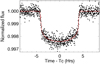 |
Fig. 5 The two TESS transits phase-folded with the model from EXOFASTv2 over plotted. |
Median values and 68% confidence intervals for HD 1397 fitted with EXOFASTv2, including two Keplerians, of which the 42-day period one tracks stellar activity.
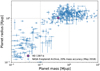 |
Fig. 6 Mass and radius of the known population of Exoplanets with HD 1397b over-plotted. Only planets with mass known to 20% or better are included. |
Acknowledgements
We thank the Swiss National Science Foundation (SNSF) and the Geneva University for their continuous support to our planet search programs. This work has been in particular carried out in the frame of the National Centre for Competencein Research “PlanetS” supported by the Swiss National Science Foundation (SNSF). This publication makes use of The Data& Analysis Center for Exoplanets (DACE), which is a facility based at the University of Geneva (CH) dedicated to extrasolar planets data visualisation, exchange and analysis. DACE is a platform of the Swiss National Centre of Competence in Research (NCCR) PlanetS, federating the Swiss expertise in Exoplanet research. The DACE platform is available at https://dace.unige.ch. We acknowledge the use of TESS Alert data, which is currently in a beta test phase, from the TESS Science Office and at the TESS Science Processing Operations Center. Funding for the TESS mission is provided by NASA’s Science Mission directorate. This work has made use of data from the European Space Agency (ESA) mission Gaia (https://www.cosmos.esa.int/gaia), processed by the Gaia Data Processing and Analysis Consortium (DPAC, https://www.cosmos.esa.int/web/gaia/dpac/consortium). Funding for the DPAC has been provided by national institutions, in particular the institutions participating in the Gaia Multilateral Agreement. This study was in part based on observations collected at the European Southern Observatory under ESO programme 0102.C-0503(A). MINERVA-Australis is supported by Australian Research Council LIEF Grant LE160100001, Discovery Grant DP180100972, Mount Cuba Astronomical Foundation, and institutional partners University of Southern Queensland, MIT, Nanjing University, George Mason University, University of Louisville, University of California Riverside, University of Florida, and University of Texas at Austin.
References
- Addison, B., Wright, D. J., Wittenmyer, R. A., et al. 2019, PASP, submitted [arXiv:1901.11231] [Google Scholar]
- Anderson, D. R., Collier Cameron, A., Delrez, L., et al. 2017, A&A, 604, A110 [NASA ADS] [CrossRef] [EDP Sciences] [Google Scholar]
- Anglada-Escudé, G., & Butler, R. P. 2012, ApJS, 200, 15 [NASA ADS] [CrossRef] [Google Scholar]
- Azizi, F., & Mirtorabi, M. T. 2018, MNRAS, 475, 2253 [NASA ADS] [CrossRef] [Google Scholar]
- Boisse, I., Moutou, C., Vidal-Madjar, A., et al. 2009, A&A, 495, 959 [NASA ADS] [CrossRef] [EDP Sciences] [Google Scholar]
- Boisvert, J. H., Nelson, B. E., & Steffen, J. H. 2018, MNRAS, 480, 2846 [NASA ADS] [CrossRef] [Google Scholar]
- Bowler, B. P., Johnson, J. A., Marcy, G. W., et al. 2010, ApJ, 709, 396 [NASA ADS] [CrossRef] [Google Scholar]
- Brahm, R., Espinoza, N., Jordán, A., et al. 2018, AJ, submitted [arXiv:1811.02156] [Google Scholar]
- Charbonneau, D. 2003, in Scientific Frontiers in Research on Extrasolar Planets, eds. D. Deming & S. Seager, ASP Conf. Ser., 294, 449 [NASA ADS] [Google Scholar]
- Cheetham, A., Ségransan, D., Peretti, S., et al. 2018, A&A, 614, A16 [NASA ADS] [CrossRef] [EDP Sciences] [Google Scholar]
- Choi, J., Dotter, A., Conroy, C., et al. 2016, ApJ, 823, 102 [NASA ADS] [CrossRef] [Google Scholar]
- Díaz, R. F., Cincunegui, C., & Mauas, P. J. D. 2007, MNRAS, 378, 1007 [NASA ADS] [CrossRef] [Google Scholar]
- Dotter, A. 2016, ApJS, 222, 8 [NASA ADS] [CrossRef] [Google Scholar]
- Eastman, J. 2017, Astrophysics Source Code Library [record ascl:1710.003] [Google Scholar]
- Eastman, J., Gaudi, B. S., & Agol, E. 2013, PASP, 125, 83 [NASA ADS] [CrossRef] [Google Scholar]
- Ford, E. B. 2006, ApJ, 642, 505 [NASA ADS] [CrossRef] [Google Scholar]
- Ford, E. B., & Rasio, F. A. 2008, ApJ, 686, 621 [NASA ADS] [CrossRef] [Google Scholar]
- Frink, S., Quirrenbach, A., Fischer, D., Röser, S., & Schilbach, E. 2001, PASP, 113, 173 [NASA ADS] [CrossRef] [Google Scholar]
- Gaia Collaboration (Brown, A. G. A., et al.) 2018, A&A, 616, A1 [NASA ADS] [CrossRef] [EDP Sciences] [Google Scholar]
- Gandolfi, D., Barragan, O., Livingston, J., et al. 2018, A&A, 619, L10 [NASA ADS] [CrossRef] [EDP Sciences] [Google Scholar]
- Gelman, A., Carlin, J. B., Stern, H. S., & Rubin, D. B. 2003, Bayesian Data Analysis, 2nd edn. (London: Chapman & Hall) [Google Scholar]
- Gomes da Silva, J., Santos, N. C., Bonfils, X., et al. 2011, A&A, 534, A30 [NASA ADS] [CrossRef] [EDP Sciences] [Google Scholar]
- Grunblatt, S. K., Huber, D., Gaidos, E., et al. 2017, AJ, 154, 254 [NASA ADS] [CrossRef] [Google Scholar]
- Grunblatt, S. K., Huber, D., Gaidos, E., et al. 2018, ApJ, 861, L5 [NASA ADS] [CrossRef] [Google Scholar]
- Halbwachs, J. L., Mayor, M., & Udry, S. 2005, A&A, 431, 1129 [NASA ADS] [CrossRef] [EDP Sciences] [Google Scholar]
- Høg, E., Fabricius, C., Makarov, V. V., et al. 2000, A&A, 355, L27 [Google Scholar]
- Huang, C. X., Burt, J., Vanderburg, A., et al. 2018, ApJ, 868, L39 [NASA ADS] [CrossRef] [Google Scholar]
- Jackson, B., Miller, N., Barnes, R., et al. 2010, MNRAS, 407, 910 [NASA ADS] [CrossRef] [Google Scholar]
- Jenkins, J. M. 2002, ApJ, 575, 493 [NASA ADS] [CrossRef] [Google Scholar]
- Jenkins, J. M. 2017, Kepler Data Processing Handbook: Overview of the Science Operations Center, Tech. rep [Google Scholar]
- Jenkins, J. M., Twicken, J. D., McCauliff, S., et al. 2016, Proc. SPIE, 9913, 99133E [Google Scholar]
- Jenkins, J. M., Tenenbaum, P., Seader, S., et al. 2017, Kepler Data Processing Handbook: Transiting Planet Search, Tech. rep [Google Scholar]
- Johnson, J. A., Aller, K. M., Howard, A. W., & Crepp, J. R. 2010, PASP, 122, 905 [NASA ADS] [CrossRef] [Google Scholar]
- Jones, M. I., Jenkins, J. S., Rojo, P., & Melo, C. H. F. 2011, A&A, 536, A71 [NASA ADS] [CrossRef] [EDP Sciences] [Google Scholar]
- Jones, M. I., Jenkins, J. S., Bluhm, P., Rojo, P., & Melo, C. H. F. 2014, A&A, 566, A113 [NASA ADS] [CrossRef] [EDP Sciences] [Google Scholar]
- Kane, S. R., & Raymond, S. N. 2014, ApJ, 784, 104 [NASA ADS] [CrossRef] [Google Scholar]
- Kane, S. R., Howell, S. B., Horch, E. P., et al. 2014, ApJ, 785, 93 [NASA ADS] [CrossRef] [Google Scholar]
- Kane, S. R., Wittenmyer, R. A., Hinkel, N. R., et al. 2016, ApJ, 821, 65 [NASA ADS] [CrossRef] [Google Scholar]
- Knutson, H. A., Charbonneau, D., Allen, L. E., et al. 2007, Nature, 447, 183 [NASA ADS] [CrossRef] [PubMed] [Google Scholar]
- Kreidberg, L., Bean, J. L., Désert, J.-M., et al. 2014, ApJ, 793, L27 [NASA ADS] [CrossRef] [Google Scholar]
- Kunitomo, M., Ikoma, M., Sato, B., Katsuta, Y., & Ida, S. 2011, ApJ, 737, 66 [NASA ADS] [CrossRef] [Google Scholar]
- Lenzen, R., Hartung, M., Brandner, W., et al. 2003, in Instrument Design and Performance for Optical/Infrared Ground-based Telescopes, eds. M. Iye, & A. F. M. Moorwood, Proc. SPIE, 4841, 944 [NASA ADS] [CrossRef] [Google Scholar]
- Liu, F., Yong, D., Asplund, M., et al. 2018, A&A, 614, A138 [NASA ADS] [CrossRef] [EDP Sciences] [Google Scholar]
- Lopez, E. D., & Fortney, J. J. 2016, ApJ, 818, 4 [NASA ADS] [CrossRef] [Google Scholar]
- Lovis, C., Dumusque, X., Santos, N. C., et al. 2011, ArXiv e-prints [arXiv:1107.5325] [Google Scholar]
- Noyes, R. W., Hartmann, L. W., Baliunas, S. L., Duncan, D. K., & Vaughan, A. H. 1984, ApJ, 279, 763 [NASA ADS] [CrossRef] [Google Scholar]
- Queloz, D., Shao, M., & Mayor, M. 2001a, BAAS, 33, 1356 [NASA ADS] [Google Scholar]
- Queloz, D., Henry, G. W., Sivan, J. P., et al. 2001b, A&A, 379, 279 [NASA ADS] [CrossRef] [EDP Sciences] [Google Scholar]
- Reffert, S., Bergmann, C., Quirrenbach, A., Trifonov, T., & Künstler, A. 2015, A&A, 574, A116 [NASA ADS] [CrossRef] [EDP Sciences] [Google Scholar]
- Ricker, G. R., Winn, J. N., Vanderspek, R., et al. 2015, J. Astron. Telesc. Instrum., Syst., 1, 014003 [Google Scholar]
- Rousset, G., Lacombe, F., Puget, P., et al. 2003, in Adaptive Optical System Technologies II, eds. P. L. Wizinowich & D. Bonaccini, Proc. SPIE, 4839, 140 [NASA ADS] [CrossRef] [Google Scholar]
- Santos, N. C., Mayor, M., Naef, D., et al. 2002, A&A, 392, 215 [NASA ADS] [CrossRef] [EDP Sciences] [Google Scholar]
- Schlafly, E. F., & Finkbeiner, D. P. 2011, ApJ, 737, 103 [NASA ADS] [CrossRef] [Google Scholar]
- Schlegel, D. J., Finkbeiner, D. P., & Davis, M. 1998, ApJ, 500, 525 [NASA ADS] [CrossRef] [Google Scholar]
- Skrutskie, M. F., Cutri, R. M., Stiening, R., et al. 2006, AJ, 131, 1163 [NASA ADS] [CrossRef] [Google Scholar]
- Spake, J. J., Sing, D. K., Evans, T. M., et al. 2018, Nature, 557, 68 [NASA ADS] [CrossRef] [EDP Sciences] [Google Scholar]
- Stassun, K. G., & Torres, G. 2018, ApJ, 862, 61 [NASA ADS] [CrossRef] [Google Scholar]
- Suárez Mascareño, A., González Hernández, J. I., Rebolo, R., et al. 2017, A&A, 597, A108 [NASA ADS] [CrossRef] [EDP Sciences] [Google Scholar]
- Sullivan, P. W., Winn, J. N., Berta-Thompson, Z. K., et al. 2015, ApJ, 809, 77 [NASA ADS] [CrossRef] [Google Scholar]
- Swift, J. J., Bottom, M., Johnson, J. A., et al. 2015, J. Astron. Telesc. Instrum., Syst., 1, 027002 [NASA ADS] [CrossRef] [Google Scholar]
- Torres, G., Andersen, J., & Giménez, A. 2010, A&ARv, 18, 67 [Google Scholar]
- Trifonov, T., Kürster, M., Zechmeister, M., et al. 2017, A&A, 602, L8 [NASA ADS] [CrossRef] [EDP Sciences] [Google Scholar]
- Twicken, J. D., Chandrasekaran, H., Jenkins, J. M., et al. 2010, in Software and Cyberinfrastructure for Astronomy, Proc. SPIE, 7740, 77401U [NASA ADS] [CrossRef] [Google Scholar]
- Twicken, J. D., Catanzarite, J. H., Clarke, B. D., et al. 2018, PASP, 130, 064502 [NASA ADS] [CrossRef] [Google Scholar]
- Vanderspek, R., Huang, C. X., Vanderburg, A., et al. 2019, ApJ, 871, L24 [NASA ADS] [CrossRef] [Google Scholar]
- Veras, D. 2016, R. Soc. Open Sci., 3, 150571 [NASA ADS] [CrossRef] [Google Scholar]
- Villaver, E., & Livio, M. 2009, ApJ, 705, L81 [NASA ADS] [CrossRef] [Google Scholar]
- Villaver, E., Livio, M., Mustill, A. J., & Siess, L. 2014, ApJ, 794, 3 [NASA ADS] [CrossRef] [Google Scholar]
- Wang, S., Jones, M., Shporer, A., et al. 2019, AJ, 157, 51 [NASA ADS] [CrossRef] [Google Scholar]
- Williams, P. K. G., Charbonneau, D., Cooper, C. S., Showman, A. P., & Fortney, J. J. 2006, ApJ, 649, 1020 [NASA ADS] [CrossRef] [Google Scholar]
- Wittenmyer, R. A., Endl, M., Wang, L., et al. 2011, ApJ, 743, 184 [NASA ADS] [CrossRef] [Google Scholar]
- Wittenmyer, R. A., Wang, S., Horner, J., et al. 2013, ApJS, 208, 2 [NASA ADS] [CrossRef] [Google Scholar]
- Wittenmyer, R. A., Jones, M. I., Zhao, J., et al. 2017a, AJ, 153, 51 [NASA ADS] [CrossRef] [Google Scholar]
- Wittenmyer, R. A., Jones, M. I., Horner, J., et al. 2017b, AJ, 154, 274 [NASA ADS] [CrossRef] [Google Scholar]
- Wright, E. L. Eisenhardt, P. R. M., Mainzer, A. K., et al. 2010, AJ, 140, 1868 [NASA ADS] [CrossRef] [Google Scholar]
- Wyttenbach, A., Lovis, C., Ehrenreich, D., et al. 2017, A&A, 602, A36 [NASA ADS] [CrossRef] [EDP Sciences] [Google Scholar]
- Yee, S. W., Petigura, E. A., & von Braun, K. 2017, ApJ, 836, 77 [NASA ADS] [CrossRef] [Google Scholar]
- Yi, S., Demarque, P., Kim, Y.-C., et al. 2001, ApJS, 136, 417 [NASA ADS] [CrossRef] [Google Scholar]
- Zechmeister, M., & Kürster, M. 2009, A&A, 496, 577 [NASA ADS] [CrossRef] [EDP Sciences] [Google Scholar]
- Zinn, J. C., Pinsonneault, M. H., Huber, D., & Stello, D. 2018, ApJ, submitted [arXiv:1805.02650] [Google Scholar]
The independent study conducted by Brahm et al. (2018), submitted on the same day as this work, also presents the discovery of HD 1397b.
All Tables
Median values and 68% confidence intervals for HD 1397 fitted with EXOFASTv2, including two Keplerians, of which the 42-day period one tracks stellar activity.
All Figures
|
Fig. 1 Timeseries of the CORALIE and MINERVA-Australis RVs with the EXOFASTv2 two Keplerian model over-plotted in red. |
| In the text | |
|
Fig. 2 Sensitivity curve from NaCo AO imaging at Br-γ. The inset image is 3 arcsec on either side. |
| In the text | |
|
Fig. 3 Time series of the Hα index (top panel), Ca II H&K S-index (middle left panel), FWHM (middle right panel), bisector span (bottom left panel) and He I index (bottom right panel) for the CORALIE spectra. The red lines show the best fit to the data. |
| In the text | |
|
Fig. 4 SED fitting of HD 1397 as produced by EXOFASTv2. The sources of the broad band photometry is detailed in Table 2. |
| In the text | |
|
Fig. 5 The two TESS transits phase-folded with the model from EXOFASTv2 over plotted. |
| In the text | |
|
Fig. 6 Mass and radius of the known population of Exoplanets with HD 1397b over-plotted. Only planets with mass known to 20% or better are included. |
| In the text | |
Current usage metrics show cumulative count of Article Views (full-text article views including HTML views, PDF and ePub downloads, according to the available data) and Abstracts Views on Vision4Press platform.
Data correspond to usage on the plateform after 2015. The current usage metrics is available 48-96 hours after online publication and is updated daily on week days.
Initial download of the metrics may take a while.