| Issue |
A&A
Volume 623, March 2019
|
|
|---|---|---|
| Article Number | A149 | |
| Number of page(s) | 10 | |
| Section | Cosmology (including clusters of galaxies) | |
| DOI | https://doi.org/10.1051/0004-6361/201832673 | |
| Published online | 22 March 2019 | |
GALEX colours of quasars and intergalactic medium opacity at low redshift
1
Aix Marseille Univ., CNRS, LAM, Laboratoire d’Astrophysique de Marseille, Marseille, France
e-mail: jean-michel.deharveng@lam.fr
2
Sirius Environmental, 1478 N.Altadena Dr, Pasadena, CA 901107, USA
Received:
19
January
2018
Accepted:
17
February
2019
Aims. The distribution of neutral hydrogen in the intergalactic medium (IGM) is currently explored at low redshift by means of UV spectroscopy of quasars. We propose here an alternative approach based on UV colours of quasars as observed from GALEX surveys. We built a NUV-selected sample of 9033 quasars with (FUV−NUV) colours. The imprint of HI absorption in the observed colours is suggested qualitatively by their distribution as a function of quasar redshift.
Methods. Because broad band fluxes lack spectral resolution and are sensitive to a large range of HI column densities a Monte Carlo simulation of IGM opacity is required for quantitative analysis. It was performed with absorbers randomly distributed along redshift and column density distributions. The column density distribution was assumed to be a broken power law with index β1 (1015 cm−2 < NHI < 1017.2 cm−2) and β2 (1017.2 cm−2 < NHI < 1019 cm−2). For convenience the redshift distribution is taken proportional to the redshift evolution law of the number density of Lyman limit systems (LLS) per unit redshift as determined by existing spectroscopic surveys. The simulation is run with different assumptions on the spectral index αν of the quasar ionising flux.
Results. The fits between the simulated and observed distribution of colours require an LLS redshift density larger than that derived from spectroscopic counting. This result is robust in spite of difficulties in determining the colour dispersion other than that due to neutral hydrogen absorption. This difference decreases with decreasing αν (softer ionising quasar spectrum) and would vanish only with values of αν which are not supported by existing observations.
Conclusions. We provide arguments to retain αν = −2, a value already extreme with respect to those measured with HST/COS. Further fitting of power law index β1 and β2 leads to a higher density by a factor of 1.7 (β1 = −1.7, β2 = −1.5), possibly 1.5 (β1 = −1.7, β2 = −1.7). Beyond the result in terms of density the analysis of UV colours of quasars reveals a tension between the current description of IGM opacity at low z and the published average ionising spectrum of quasars.
Key words: intergalactic medium / ultraviolet: general / quasars: general
© J.-M. Deharveng et al. 2019
 Open Access article, published by EDP Sciences, under the terms of the Creative Commons Attribution License (http://creativecommons.org/licenses/by/4.0), which permits unrestricted use, distribution, and reproduction in any medium, provided the original work is properly cited.
1. Introduction
Decades of quasar absorption line studies have provided a wealth of information on the column density and redshift distributions of the neutral hydrogen pockets surviving in the nearly completely ionised intergalactic medium (IGM). These distribution functions have become basic ingredients for the evaluation of the IGM opacity to ionising radiation, a crucial link between the emissivity of the sources of ionising photons and the intensity of the ionising ultraviolet background radiation (e.g. Haardt & Madau 1996, 2012). At large redshifts (≳3), the sources contributing to the hydrogen ionisation at a given point in the IGM are essentially local and the transfer of ionising photons can be reduced to a mean free path term (e.g. Madau et al. 1999; Schirber & Bullock 2003; Faucher-Giguère et al. 2008; Becker & Bolton 2013). The mean free path depends on the properties of systems of optical depth near unity, usually referred as Lyman limit systems (LLSs). In addition, the mean free path to ionising photons can be now directly measured through composite quasar spectra (e.g. Prochaska et al. 2009; O’Meara et al. 2013; Fumagalli et al. 2013; Worseck et al. 2014).
The situation at low redshift (z < 2) deserves special attention for two reasons. For one, the mean free path to ionising radiation becomes very large (e.g. Fumagalli et al. 2013) and the simplification described above is no more valid. Second, the spectroscopic surveys of low-redshift LLSs, based on the identification of the Lyman break at 912 Å require space-based ultraviolet observations which have been scarce. This, in combination with the intrinsically low frequency of LLSs at low redshift, explains the limited size of available samples. Following the pioneering work of Tytler (1982) using IUE, Stengler-Larrea et al. (1995) have homogenised the early observations with those obtained from the first spectrographs of HST, ending with 11 LLSs in the redshift bin (0.36, 1.1). Songaila & Cowie (2010) have added nine LLSs in the redshift bin (0.58, 1.24) from the observations of 50 quasars with the GALEX grism spectrograph. Ribaudo et al. (2011) have performed an extensive analysis of archival HST quasar spectra (including from STIS), resulting in 31 LLSs (τ > 1) in their two lowest redshift bins (0.255, 1.060), (1.060, 1.423). More recently, O’Meara et al. (2013) have analysed the incidence of LLS in 71 quasars observed with the low dispersion modes of HST/ACS and HST/WFC3; they report 19 LLSs (τ > 1) at z < 2 but with an average redshift of about 1.8 and the bulk of statistical power at 2 < z < 2.5.
The Lyman break which can be identified in relatively noisy and low resolution spectra is also expected to leave a trace in the UV colours of quasars, opening the possibility to retrieve information on the distribution of LLSs and more generally HI in the low redshift IGM. Samples of UV colours of quasars, as obtained from GALEX surveys, can be much larger and less biased than the spectroscopic samples described above. The paper is organised as follows. In the second section we describe how a sample of quasars with GALEX UV colours is built and how the presence of absorbers is contributing the dispersion observed in the colour distribution. In the third section we review the challenges for extracting quantitative information from the UV colour distribution. In the fourth section we propose a simple model, including a Monte Carlo calculation of the IGM opacity to ionising photons, to predict colour distribution from a limited set of parameters. In the fifth section we run the simulation in different redshift bins, forward modelling the input parameters by comparison with observations.
2. Hints for IGM opacity in UV colours
2.1. A sample of quasars with GALEX ultraviolet colours
The GALEX instrument provides a (FUV−NUV) colour from imaging in two ultraviolet bands, the FUV (1350–1750 Å) and NUV (1750–2750 Å), with  –
– resolution and
  field of view. The two bands are obtained simultaneously using a dichroic beam splitter. The observations are performed through three types of survey, the All-sky Imaging Survey (AIS) with typical exposure times of 100 s, the Medium Imaging Survey (MIS) with typical exposure times of 1500 s, the Deep Imaging Survey (DIS) with typical exposure times of 30 ks. A full description of the instrument and the mission is given by Martin et al. (2005), Morrissey et al. (2005, 2007).
A large sample of quasars with ultraviolet colours has been obtained by cross-correlating the SDSS Data Release 7 (DR7) quasar catalogue with the GALEX catalogue of UV sources, corresponding essentially to the data release GR4/GR5. The quasar catalogue (Schneider et al. 2010) contains 105 783 spectroscopically confirmed quasars. A maximum match radius of  was adopted, slightly above the recommendation of Morrissey et al. (2007) based on the study of GALEX astrometry and similar to the value adopted by Trammell et al. (2007) in a previous study of the UV properties of SDSS-selected quasars. Larger match radii have been tested and discussed in the different context of GALEX FUV selection of high-redshift quasars by Syphers et al. (2009) and Worseck & Prochaska (2011). Our concern here is avoiding non quasar UV source rather than missing one line of sight since a miss, provided it is not related to neutral hydrogen absorption, is not expected to introduce any selection effect. As we are interested by the variations of the (FUV−NUV) colour that might be caused by absorber Lyman break within the GALEX bands we have limited ourselves to z < 1.9. A more conservative limit will be adopted later in the analysis for the purpose of reducing selection effects. In order to avoid any risk of limitation in the astrometry or the photometry at the edge of the GALEX field of view, the useful field was limited to a radius of
  . More than one UV source may be obtained within the
  match radius, most often in the case of quasars imaged in multiple GALEX exposures. Because of the poor astrometry at low signal to noise ratio, the closest source is not necessarily the one with the highest effective exposure time in the NUV. In order to overcome this issue and to retain significant NUV flux we have applied a threshold of 900 s to the NUV exposures before selecting the nearest source. This exposure time of 900 s corresponds to a clear dip in the distribution of exposure times between the AIS and the MIS surveys. For homogeneity we have applied a similar cut at 800 s to the FUV exposures. This results in a NUV-selected sample of 12 038 quasars with AB magnitudes ranging from 15.7 to 24.8. The (FUV−NUV) colours are calculated for the 9033 quasars also detected in the FUV. No correction for Galactic extinction is applied because, under current assumptions, the colour correction is only one third of the E(B − V) colour excess (e.g. Wyder et al. 2005).
2.2. The effect of absorbers on the UV colour distribution
The (FUV−NUV) colours of the 9033 quasars detected in both GALEX bands are displayed in Fig. 1 as a function of the emission redshift. This plot is similar to one of those obtained by Trammell et al. (2007) in a previous study of the UV properties of SDSS-selected quasars. To deal with the 3005 quasars not detected in the FUV we have observed that the faintest FUV detections reach an (AB) magnitude of 24, rather flat from exposure times of 800 s to 5000 s and slowly increasing to 25 for longer exposures. As the exposure times longer than 5000 s make less than 5% of those with quasar undetected in the FUV we have adopted 24 as a limiting magnitude to display lower limit colours of the 3005 quasars not detected in the FUV in Fig. 2.
 |
Fig. 1. (FUV−NUV) colours of 9033 quasars from the SDSS DR7 detected in both GALEX bands, as a function of their emission redshift. |
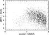 |
Fig. 2. Lower limit (FUV−NUV) colours of 3005 quasars from the SDSS DR7 detected only in the NUV GALEX band, as a function of their emission redshift. |
These two first figures are best understood with the details of the GALEX bands which are shown Fig. 3. When the emission redshift ze increases from 0.45 to 0.95 the probability of a Lyman break within the FUV band increases regularly as a function of the difference ze − 0.45. The fraction of red quasars off the main locus of points follows a similar trend in Fig. 1. There is not yet any real FUV dropout in agreement with the relatively small number of lower limit colours in Fig. 2. Beyond ze = 0.95 the trend flattens since an increasing fraction of quasars may have a Lyman break longward of the FUV band and go undetected, as seen in Fig. 2.
 |
Fig. 3. Effective area (counts cm2 photon−1) of the FUV and NUV GALEX bandpasses (Morrissey et al. 2007). The vertical (red) tick marks indicate the position with respect to the bandpasses of the Lyman break at redshifts 0.45, 0.95 and 1.35. |
2.3. Comparison with samples of spectroscopically identified LLSs
In order to support our view that the red colours of quasars may indicate the presence of neutral hydrogen absorption we have looked at the distribution of GALEX UV colour vs. emission redshift in existing samples with spectroscopically identified LLSs at low redshift.
We have first used the GALEX grism spectrograph observations of 50 quasars with 0.8 < ze < 1.3 by Songaila & Cowie (2010). The UV colours have been found from MAST (Mikulski Archive for Space Telescopes) and are displayed in Fig. 4. Of the nine quasars with a LLS spectroscopically identified by Songaila & Cowie (2010), eight have colours significantly redder than the quasars without LLS, including the one with a lower limit colour which is not a FUV dropout (LLS at z = 0.82).
 |
Fig. 4. (FUV−NUV) GALEX colours as a function of emission redshift for the 50 quasars observed with GALEX grism spectrograph by Songaila & Cowie (2010). One lower limit colour (source GALEX 1712+6007) is indicated with a red triangle. All nine quasars circled in green colour (including the lower limit) have spectroscopically identified LLSs. Their LLS redshifts are all at z < 0.95 within the FUV band, except z = 1.11 for the reddest object GALEX1418+5223 which does not appear as a FUV dropout. |
Second, we have used the analysis by Ribaudo et al. (2011) of the population of LLSs at low redshift from archival HST spectral observations with the Faint Object Spectrograph (FOS) and the Space Telescope Imaging Spectrograph (STIS). The GALEX UV colours have been searched for all the quasars with redshift ze < 1.85 in their sample used for LLS statistics (their Table 3). They are displayed in Fig. 5 for 112 quasars along with 49 quasars with only lower limit colour (no detection in the FUV). The quasars with a spectroscopically identified LLS (from their Table 4) are circled, except for four of them with a Lyman break at too low redshifts to be included in the FUV band. The vast majority of quasars with red colours, that is (FUV−NUV) larger than about two, and among them a significant number of lower limits, have spectroscopically identified LLSs while those bluer have none. Among the 13 quasars circled with (FUV−NUV) < 2 we have either objects classified as PLLSs (partial Lyman Limit System, τ < 1) by Ribaudo et al. (2011) or an absorption redshift zLLS < 0.66; both situations come with less absorption in the GALEX FUV band.
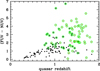 |
Fig. 5. (FUV−NUV) GALEX colours (black dots) and lower limit colours (red triangles) as a function of emission redshift for the quasar sample used by Ribaudo et al. (2011) for studying LLS statistics. Quasars circled in green colour (including the lower limits) have spectroscopically identified LLSs. The vast majority of quasars with (FUV−NUV) > 2 have spectroscopically identified LLSs. |
3. Interplay between UV colours and IGM opacity
Although the distributions of GALEX UV colours displayed in the previous sub-sections illustrate beyond doubt the impact of LLSs (and more generally neutral hydrogen absorption) on these colours, there are many difficulties for extracting quantitative information.
First of all, other factors contribute to the dispersion/reddening of UV quasar colours. In addition to photometric uncertainties, there is a natural dispersion of intrinsic quasar colours. Although the spectral energy distribution of quasars display a relatively consistent mean successfully approximated by power laws, a significant dispersion is still present. We need to examine how the spectral energy distributions of quasars can be described in the rest-frame spectral range relevant to the GALEX colours and redshift range of interest here and whether it is possible to disentangle information on the absorbers from the uncertainties in the flux distribution.
A related aspect is the large number of lower limit colours coming with the quasar undetected in the FUV band. In the absence of any absorption the quasars are already red, at a typical (FUV−NUV) colour of about one. With a median NUV magnitude of 22.4 over the full sample, a number of quasars go undetected in the FUV with only a modest reddening (typically 1.6 mag associated to a FUV limiting magnitude of 25). In these conditions many lower limit colours are not indicative of true FUV dropouts.
Another obvious difficulty in the interpretation of photometric data is the lack of spectral resolution which prevents determination of any absorption redshift and results in a degeneracy between absorption redshift and column density. Any colour significantly redder than the average trend in Fig. 1 and potentially revealing neutral hydrogen absorption may be caused by different combinations of absorption redshift and absorption strength. This is a basic difference with a spectroscopic approach which provides a list of well defined absorbers at specific redshifts and with a uniform optical depth limit (e.g. larger than 1 or 2) that can be translated into a distribution law of LLSs (i.e. number of LLS per unit redshift as a function of z). Here, the UV colour is influenced not only by the absorbers that are usually identified as LLSs (optical depth larger than 1 or HI column density NHI ≥ 1017.2 cm−2 ) but also by an increasing number of absorbers with NHI < 1017.2 cm−2. In contrast to counting a few well identified optically thick clouds, we are challenged here by an opacity problem caused by a large population of absorbers. This bears resemblance to the direct evaluation of mean free path to ionisation radiation through the analysis of stacked spectra by O’Meara et al. (2013) and Worseck et al. (2014).
In the same vein as the redshift vs. absorption strength degeneracy due to the lack of spectral resolution, the photometric approach is unable to distinguish absorbers lying close to the quasars which are usually excluded in spectroscopic surveys (e.g. Proximate LLSs in Prochaska et al. 2010).
Beyond ze = 0.95, LLSs may appear in the NUV band and be responsible for a decrease of the quasars NUV flux depending on the HI column density of the LLS and its position in the band. The resulting sample bias increases rapidly with redshift and requires a cut in the redshift ze for any quantitative analysis. Some average numbers may be derived from the average redshift density of 0.82 LLS reported in the range (1.060, 1.423) by Ribaudo et al. (2011). For a sample of about 600 quasars as in our observations, we get about 144 LLSs in the NUV band up to ze < 1.3, with an absorption of as much as 0.27 of the NUV flux of the quasars. Up to ze < 1.4 we get about 192 LLSs with an absorption of as much as 0.4 of the NUV flux. A redshift cut at ze < 1.35 would therefore keep sample bias within acceptable limits for quantitative analysis.
4. Modelling the distribution of quasar UV colours
To recover quantitative information from the observed dispersion of the UV colour distribution, we have generated Monte Carlo quasar spectra randomly imprinted with IGM absorption from the observed statistical properties of redshift and column density distributions of neutral hydrogen. Folded through the GALEX bandpasses, these spectra provide a large set of colours to be compared with the observed UV colour distribution. We review in the following sub-sections the physical quantities entering the calculations and expected to be constrained in this comparison.
4.1. Quasar spectral energy distribution
The first step of the simulation is to adopt a representative quasar spectral energy distribution over the rest frame wavelength range 550 Å–2800 Å that is shifted over the GALEX bandpasses for quasars with ze < 1.35. The rest-frame continuum of quasars is usually described by power laws Fν ∝ ναν or Fλ ∝ λαλ with αν = −(αλ + 2) (e.g. Shull et al. 2012).
At wavelengths longer than about 1100 Å, there is a consensus on the spectral index which consequently will not be retained as a parameter to be optimised through the simulation. In addition as emission lines may play a role in the quasar colours, we have not chosen an average index but preferred to adopt the composite spectrum of Vanden Berk et al. (2001). Incidentally, this composite spectrum can be approximated by a power law index of −0.44 above 1200 Å (Vanden Berk et al. 2001). In contrast, the αν index in the EUV domain (< 912 Å) should be an essential parameter of the simulation since it is in this wavelength range that the interplay between the quasar ionising flux continuum and the continuum absorption by neutral hydrogen clouds is expected to change the most the GALEX broadband fluxes. A number of αν index values have already been reported from UV spectroscopic observations of bright, low-z targets. Zheng et al. (1997) obtain αν = −1.8 (radio-quiet sample only) from HST/FOS and Telfer et al. (2002)αν = −1.57 ± 0.17 (radio-quiet), −1.96 ± 0.12 (radio-loud) from HST/FOS/GHRS/STIS. These values are challenged by αν = −0.56 from FUSE observations (Scott et al. 2004) but from GALEX spectroscopy Barger & Cowie (2010) find values of −1.76 and −2.01 in good agreement with the earlier HST determinations of Zheng et al. (1997) and Telfer et al. (2002). More recent results have not clarified the situation. Shull et al. (2012) and Stevans et al. (2014) report αν = −1.41 ± 0.15 from HST/COS observations. The first quasar stacked spectrum at z ∼ 2.4 from HST/WFC3 (Lusso et al. 2015) has confirmed the most negative values but a value αν = −0.72 ± 0.26, in line with that from FUSE, has been recently given from new HST/COS observations and analysis (Tilton et al. 2016). The αν index (< 912 Å) is clearly a parameter to be optimised in our simulation.
One area of difficulty, especially for our purpose of integration into the GALEX bandpasses, is the transition zone between the composite spectrum of Vanden Berk et al. (2001) and the softening expected in the EUV domain according to most of the values in the references above. A comparison with the composite spectrum of Shull et al. (2012) suggests to stop the composite spectrum of Vanden Berk et al. (2001) below 1190 Å once the Lyα line has been fully covered and to start the αν power law continuum only below about 1000 Å. Between, we have used an intermediate power law continuum (Fig. 6). By folding the resulting complete spectral energy distribution into the GALEX bandpasses, we have determined an index ∼ − 1.4 as best matching the observed colour distribution of Fig. 1 in the domain of ze < 0.6 where the dispersion of colours is not yet affected by IGM opacity effects. This is shown in Fig. 7. This figure illustrates how the power law index of the ionising spectrum starts to affect the quasar colours above a redshift of 0.7 and is the most sensitive in the range 0.9–1.3.
 |
Fig. 6. Mean quasar spectral energy distribution adopted for the simulation displayed at redshift 0.4 (red) and 1.2 (green), superposed with the GALEX bandpasses (black dotted lines). It is composed of three parts, (i) the composite spectrum of Vanden Berk et al. (2001) above 1190 Å rest frame, (ii) a power law continuum below 1000 Å rest frame with an index αν to be varied in the simulation. It is shown here with values −1.4 (solid lines αλ = −0.6) and −2.4 (dashed lines αλ = 0.4), (iii) a power law continuum with an index −1.4 (αλ = −0.6) between 1000 Å and 1190 Å (rest frame). |
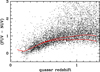 |
Fig. 7. Zoom-in of Fig. 1 with the observed (FUV−NUV) GALEX colours. Superposed in red is the colour distribution for the mean spectral energy distribution adopted for the simulation and shown in Fig. 6. Two values of the power law index αν in the wavelength range below 1000 Å rest frame have been used: −2.4 (top), −1.6 (bottom). Such a diagram was used to determine the index value between 1000 Å and 1190 Å (rest frame) matching the best the observations in the range ze < 0.6 (see text). |
4.2. IGM absorption
The second step of the simulation follows the standard practice of Monte Carlo evaluation of the intergalactic hydrogen attenuation due to photoelectric absorption and resonant scattering by Lyman transitions (e.g. Møller & Jakobsen 1990; Madau 1995; Bershady et al. 1999; Meiksin 2006; Inoue & Iwata 2008; Haardt & Madau 2012; Inoue et al. 2014). At low redshift we can concentrate on the photoelectric absorption mechanism and we have not extended the simulation to the resonant scattering by Lyman transitions. To account for this latter mechanism we have used instead the observed average transmission 1 − 0.013(1 + ze)1.54 (observed wavelength frame) reported at low redshift by Kirkman et al. (2007). We have calculated that this factor has an impact of less than 0.05 mag on the colour in nominal conditions.
We now turn to the parameters used in the Monte Carlo evaluation of the Lyman continuum absorption and, among them, the necessary limited number of those we plan to vary and constrain by fitting the output of the simulation with the observed quasar colour distribution. We adopt the current notation (e.g. O’Meara et al. 2007; Prochaska et al. 2010) for the column density distribution function f(NHI, X) giving the number of absorbers with column density NHI per dNHI interval and per absorption pathlength dX (for the moment we ignore X and the relation with the redshift). The NHI dependency of this function is usually approximated by broken power laws (e.g. Prochaska et al. 2010; Ribaudo et al. 2011; O’Meara et al. 2013) of the form  with the Ai and βi independent of redshift and linked by continuity equations at the breaking points between the different classes of absorbers.
The sub-DLAs (1019 cm−2 < NHI < 1020.3 cm−2) and DLAs (NHI ≥ 1020.3 cm−2) do not contribute much to the opacity because of their small numbers. As the column density distribution is also measured in these categories of absorbers from the damping profiles, we have therefore adopted the values (respectively β3 = −0.8 and β4 = −1.4) reported by Ribaudo et al. (2011) for the most comparable redshift range. This leaves β2 for the LLSs (1017.2 cm−2 < NHI < 1019 cm−2), β1 for the PLLSs (partial LLS, NHI < 1017.2 cm−2; the column density lower limit will be determined later) and the values A1 (or A2) as parameters to optimise in our simulation.
For the purpose of comparison with previous observations and in order to explore realistic values for matching the observed quasar colour distribution, it is highly desirable to establish the relation between our set of parameters and the density of LLSs observed from previous spectroscopic surveys. In these surveys the observable quantity is the redshift density of LLSs l(z), obtained as the ratio of the number of LLSs (usually with optical depth τ > 1) detected in a redshift interval to the total survey path contained in that redshift interval. The redshift evolution law is often parameterised as l(z) = l0(1 + z)γ. We will refer to those of Ribaudo et al. (2011), l(z) = 0.286(1 + z)1.19 (τ > 1) and Songaila & Cowie (2010), l(z) = 0.151(1 + z)1.94 displayed in Fig. 8 along with the density measurements from which they have been obtained.
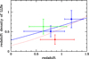 |
Fig. 8. Previous determinations at z < 1.5 of the redshift density l(z) of LLSs (τ > 1) from spectroscopic surveys: triangle (green), Stengler-Larrea et al. (1995) with the numbers reported by Songaila & Cowie (2010); solid circle (blue), Ribaudo et al. (2011); solid square (red), Songaila & Cowie (2010) from GALEX grism spectroscopy. The lines are redshift evolution laws used for comparison: the solid line (blue) is from Ribaudo et al. (2011), derived from their UV data; the dotted line (red) is from Songaila & Cowie (2010), based on high-redshift data and a combination of their GALEX data and those of Stengler-Larrea et al. (1995). |
The quantity l(z) is related to l(X), the density of LLSs per unit pathlength X, by (e.g. Ribaudo et al. 2011; O’Meara et al. 2013)

where

and

l(X) is the zeroth moment of the column density function f(NHI, X) and with the broken power laws approximating this function, writes as

With the relations above and l(X) almost constant at low redshift, we may calculate the average number of LLS absorbers (NHI > 1017.2 cm−2) along a line of sight up to a redshift ze, as (assuming ΩΛ = 0.7 and Ωm = 0.3)

Substituting the value of l(X)NHI > 1017.2 cm−2 from the integration on the power laws into the last equation and comparing with the other calculation of the number of LLSs given by

provides a link between the set of parameters to optimise and the LLS density measured by Songaila & Cowie (2010) and Ribaudo et al. (2011). This allows us to compare the constraints from our photometric approach with the data from previous spectroscopic surveys.
If we assume that the shape of the redshift evolution as a function of z used for LLSs may be extended in the domain of PLLSs, the above equations may be extended down to lower column density with the parameters A1 and β1. They may be used to determine the lowest column density NHI, lim with a significant role in the IGM Lyman continuum absorption.

and

We have used column density limits of 1014 cm−2 to 1015 cm−2 (domain of transition between the Ly-α forest and the PLLSs) and current values of β1 and β2 in the two equations above to run the opacity calculation described in the following subsection. Moving the limit from 1015 cm−2 to 1014 cm−2 would increase the total number of absorbers by a factor of about 4.9 but only decrease the average transmitted FUV to NUV flux ratio by less than 0.002. For all practical purpose the range of column densities above the limit of 1015 cm−2 is responsible for the totality of neutral hydrogen absorption and will be used in the following Monte Carlo opacity evaluation.
4.3. Monte Carlo opacity calculation
For each quasar line of sight used in our Monte Carlo opacity calculation, a number of absorbers has been pseudo-randomly generated from a Poisson distribution with, for mean parameter, the number NNHI > 1015 cm−2 obtained above for the emission redshift ze. The selected number was in turn distributed pseudo-randomly on redshift and column density according to the distribution laws l(z)=l0(1 + z)γ and  in their respective NHI domains.
An absorber of column density NHI at an absorption redshift za has an optical depth at rest wavelength λ = λ0/(1 + za) given by
τ = 6.3 × 10⁻¹⁸(λ0/(1 + za)/912)3NHI or
τ = 0 if λ0/(1+za) > 912 Å.
The total optical depth at λ0 is obtained by adding all individual absorber optical depths. The resulting transmission as a function of wavelength is then multiplied with the quasar spectral energy distribution (defined above with the spectral index αν) and provides a quasar spectrum with randomly imprinted IGM absorption. Finally an integration in the GALEX bandpasses gives the distribution of quasar UV colours resulting from our Monte Carlo opacity evaluation.
5. The optimisation process
The previous section has identified the four input parameters of our Monte Carlo simulation of the distribution of GALEX UV colours of quasars at low redshift. They are the quasar continuum spectral index αν in the EUV spectral range, the power law index of the HI column density distribution β1 in the range 1015 cm−2 < NHI < 1017.2 cm−2 and β2 in the range 1017.2 cm−2 < NHI < 1019 cm−2 and the density factor A1.
Given the factor larger than two between the LLS redshift densities determined so far by spectroscopy in the FUV range (see Fig. 8) we started the optimisation with the density factor A1 and αν expected to affect most the simulated colour histograms. The density factor A1 is calculated with the equations in Sect. 4.2 and the redshift evolution law used for the density of LLSs. After a normalisation by the density factor obtained with the evolution law adopted, it is possible to work in terms of a relative number density (1 + k) in each redshift bin. Adopting the evolution law of Ribaudo et al. (2011) this means that when k is 0.5 we have 1.5 times more LLSs than implied by their distribution law.
The parameters β1 and β2 are first set to a central value −1.5 and are expected to provide a possible fine tuning on the density factor A1 once determined. They correspond to a range of NHI where most of the opacity to hydrogen-ionising photons takes place and where the column density distribution function may be difficult to establish. In the range 1015 cm−2 < NHI < 1017.2 cm−2 (index β1) the absorbers are saturated in Lyα and, unless the Lyman break is measurable, the determination of NHI requires the use of high-order Lyman series transitions (e.g. Kim et al. 2002; Kim et al. 2013). Although of relatively low opacity individually, the absorbers contribute to the overall opacity through their number (e.g. Rudie et al. 2013). In the range 1017.2 cm−2 < NHI < 1019 cm−2 (index β2) the HI column densities can be distinguished on the basis of the Lyman breaks only at the low range extremity and the LLS density resulting from spectroscopic survey is in fact an integral on a column density function.
The emission redshift ze is a crucial quantity since the quasar intrinsic colour depends on the redshift and the number of absorbers is related to the redshift pathlength within the GALEX bandpasses whatever the random distribution of absorbers adopted. The comparison will therefore be divided into redshift intervals. Ten emission redshift bins from ze = 0.4 to 1.3, with size ze ± 0.05 and containing from 500 to 800 observed quasars are used. In each of these bins, 104 model lines of sight are usually run for each set of parameters. The distribution obtained from the simulation is scaled to the number of quasars observed within the same redshift bin (including those with only lower limit on the colours). In part because of these lower limit colours, it was found more convenient to perform the comparison and optimisation in the form of cumulative colour histograms.
5.1. Evaluation of a dispersion factor
Before we can use the randomly generated distribution of quasar UV colours for comparison with the observations, we have to add a dispersion factor to the colours that is not due to the neutral hydrogen absorption. This dispersion accounts for the combination of photometric uncertainties and a natural deviation of quasar colours from the average spectral energy distribution. In order to proceed with this dispersion in our simulation, we have added a normally-distributed random number with a mean zero and a standard deviation σ to the FUV-to-NUV flux ratio obtained for each of our quasar model line of sight. We have used the FUV-to-NUV flux ratio instead of the colour in order to account for cases with negative result and to trace them as lower limit UV colour.
The low redshift bin at ze = 0.4 where no Lyman break has yet entered the FUV GALEX band and no neutral hydrogen absorption has yet affected the colours is a natural place to determine this dispersion. In the simulation the calculated cumulative colour histogram depends only on σ and fits best the observations for σ = 0.05 (bottom panel of Fig. 9). This is consistent with the rms flux ratio dispersion of 0.047 calculated with the 528 objects in the bin ze = 0.4. The bin at ze = 0.5 can also be considered for the calibration of the dispersion factor since the hydrogen absorption contribution should remain marginal. The fit, not as good as for ze = 0.4, leads to σ = 0.06 and gives a sense on the uncertainty on our dispersion factor.
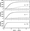 |
Fig. 9. Illustration of the fit between simulated (solid line) and observed (dotted line) cumulative colour histograms in different situations. Bottom panel: at ze = 0.4 (528 colour measurements; seven lower limits) the fit depends essentially on the dispersion factor and a value σ = 0.05 ± 0.005 is determined by the best fit. Middle panel: fit obtained at ze = 1.0 with k = 0.6 and αν = −2.4. Top panel: fit obtained at ze = 1.2 with k = 0.9 and αν = −2. In each panel, the dashed line is for the lower limit observed colours. Whilst it is negligible in the bottom panel, this contribution increases with redshift and remains always larger than the number of objects with negative FUV flux produced by the simulation. |
We have a number of reasons for extending up to ze = 1.35 our calibration σ = 0.05 at low redshift. First, the NUV magnitude distribution is not changing very much among the 10 redshift bins (average magnitude per bin between 19.76 and 20.19) and consequently an increase of photometric uncertainty with redshift due to UV flux getting fainter is unlikely. Second, we have plotted the observed GALEX (FUV−NUV) colours as a function of their NUV magnitude in Fig. 10. Even in the case of the redshift bins 1.0–1.3 which exhibit the largest skewness as seen Fig. 1 there is no relation between the reddest and the faintest quasars. Last, the possibility that the reddest colours may be associated to objects in high galactic extinction regions has been examined. Of the 2537 quasars in Fig. 10 only 56 objects have u band Galactic extinction Au > 0.5 (Schlegel et al. 1998) with a maximum Au = 1.04. Among these latter 56 objects only seven have (FUV−NUV) > 2 while the seven with the largest Au have (FUV−NUV) < 2. There is no relation between the reddest colour and high galactic extinction regions. Incidentally, the extinction Au = 0.5 would correspond to a shift of −0.05 and 0.842 in the (FUV−NUV) and NUV magnitude respectively with the corrections of Wyder et al. (2005), AFUV = 1.584 × Au and ANUV = 1.684 × Au.
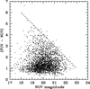 |
Fig. 10. (FUV−NUV) colour as a function of NUV magnitude for 2537 quasars in the range 0.95 < ze < 1.35. Lower limit colours of the 688 quasars undetected in the FUV are along the short-dashed line. |
Although these series of arguments support our calibration of a dispersion factor at low redshift we acknowledge that we are missing an evaluation of photometric uncertainties. This is a consequence of using colours instead of fluxes in our simulation, in order to stay away from uncertainties associated to UV luminosity functions of quasars. In the following we will therefore control on purely empirical basis how each optimization may be dependent on variations around the nominal dispersion factor of σ = 0.05.
5.2. The bin by bin optimisation
We have explored the fit between predicted and observed cumulative histograms up to the bin ze = 1.3 with steps of 0.1 in αν and k, in the ranges −2.6 < αν < −1.2 and 0 < k < 2. The steps correspond to a reasonable change that can be detected in the histogram comparison. We have proceeded quantitatively searching the minimum of the absolute sum of the differences in each colour histogram bin up to a colour of 3. Fits are not considered satisfactory if this minimum is larger than about 350.
No satisfactory fit between predicted and observed cumulative histograms is found over the redshift bins 0.6–0.9 as if the number of absorbers was not yet large enough nor the EUV spectral range sufficiently well shifted in the GALEX bandpasses for the optimal sensitivity of the method to be reached. It is also possible that the spectral index adopted to represent the typical quasar spectrum has significant dispersion in the transition zone between 1190 Å and 1000 Å. In addition we have checked that this situation is not due to slight variations of the dispersion factor σ.
Beyond redshift 0.9 where the neutral hydrogen absorption becomes prevalent satisfactory fits may be obtained when the number density increases (example in Fig. 9). This happens over a significant range of αν values. The combinations of index αν and number density (1+k) leading to these fits are collected and displayed in Fig. 11. Error bars corresponding to the precision on the determination of the fits are of the order of 0.05 and are shown (they were obtained by running 50 000 model lines of sight and using a step of 0.05 in k). These fits are obtained with the nominal value σ = 0.05. In some instances a better fit may be found with different values of σ. If the value of k is different we have extended accordingly the error bar on k as a sign of added uncertainty due to photometric dispersion. Beyond the range of αν values displayed, −2.6 < αν < −1.5, there is no satisfactory fits for all the redshift bins.
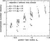 |
Fig. 11. Power law index αν and relative number density values providing a satisfying fit between the predictions and the cumulative histogram of observed colours. These are shown for 6 αν values and at each of these points the data are slightly shifted in x-direction to display the 4 redshift bins, 1.0, 1.1, 1.2 and 1.3 from left to right. A few cases where satisfying fits are obtained only with σ values different from nominal are shown as solid triangles. Open symbols show how number density values are decreased with values of β1 and β2 specified in the graph. |
For each set of index αν and number density values in Fig. 11, we have applied the Kolmogorov–Smirnov test to the two distribution functions involved in each fit and attached to observations and simulation respectively. The maximum difference between the cumulative distributions is found to vary from 0.035 to 0.105, which according to the statistical test tables and the sample size of 30 bins translates into a 95% significance level in all cases.
We have finally examined how variations of the parameters β1 and β2 affect the main trend in Fig. 11. Densities can be obtained below the main trend and are plotted as open symbols with indications of the relevant β1 and β2 values. The nominal value of dispersion σ = 0.05 has been used and error bars similar to those in the main trend are not displayed for clarity.
5.3. Results
A major result in Fig. 11 is that the simulation requires larger density of LLSs than found from previous spectroscopic determinations. We emphasise that the number density in ordinate is the fraction of absorbers in the range 1017.2 cm−2 < NHI < 1019 cm−2 normalised by the density of LLSs over the same range of HI column density obtained from the evolution law of Ribaudo et al. (2011) integrated to the appropriate redshift. Adopting the evolution law of Songaila & Cowie (2010) which shows densities lower than those of Ribaudo et al. (2011) in the redshift range of interest would lead to larger overdensities. Using an arbitrary evolution law is beyond the scope of our method.
The required overdensity is dependent on the spectral index αν of the quasar ionising spectrum and decreases when the index decreases and gets softer than the range of usually reported values (see Sect. 4.1). This effect is stronger than the uncertainties on the dispersion σ. The dependence on the spectral index does not come as a surprise since the evaluation of colours has to use an intrinsic quasar spectrum for reference; less ionising flux from quasar should require less neutral hydrogen absorption to produce the same colour dispersion. This is illustrated by the two options of αν plotted in Fig. 7. At αν > −2 we are faced to an unwanted situation with k values changing significantly with the redshift bin. This will be discussed in light of all the constraints on αν and the number density.
Figure 11 shows also the lower overdensities values reached after optimisation of the β1 and β2 parameters, about 1.7 (αν = −2) or 1.4 (αν = −2.4) with β1 decreased to about −1.7. This value of β1 is in agreement with the value −1.65 reported by Kim et al. (2002, 2013), and Rudie et al. (2013). Lower overdensities at about 1.5 (αν = −2) or 1.2 (αν = −2.4) may be obtained with β2 decreased also to about −1.7. However, the latter value is not consistent with a flattening of the column density distribution at NHI > 1017.2 cm−2 reported by most of the observations (e.g. Prochaska et al. 2010) and simulations (Altay et al. 2011).
6. Discussion
The optimisation of the power law indices β1 and β2 of the HI column density distribution has eased but not solved the tension between the results of our approach and existing density evaluations based on spectroscopy. In order to determine which combination of values to adopt from our approach we need to examine the existing constraints on the ionising quasar spectrum (αν index) and the density of LLSs.
6.1. Ionising quasar spectrum (αν index)
There is a large spread in the average power law spectral index reported for the ionising spectrum of quasars from about −2 to −0.56 (see Sect. 4.1). This range of values excludes the lowest overdensities obtained for αν < −2. Constraining the overdensities within reasonable values and avoiding the unwanted dispersion with redshift observed at large αν in Fig. 11 would require to stay close to this limit αν = −2. This is in contrast with the distribution in spectral index obtained from 159 HST/COS AGN by Stevans et al. (2014) with few objects with αν < −2.
A possible explanation has perhaps to do with the duality of the average spectral index αν. On one hand, especially in the case of simulation, the index is for the total ionising flux. On the other hand the index refers only to the UV continuum of the quasar light in which case the spectral resolution is crucial for continuum placement in presence of EUV absorption and emission lines (e.g. Stevans et al. 2014). In these conditions an αν index of about −2, close to determinations earlier than those taking advantage of the high spectral resolution of HST/COS, might be appropriate.
6.2. LLSs density
While the spectroscopic determination of the density of LLSs does not include those too close to the quasar (usually within 3000 km s−1), our approach coupled with opacity model does not distinguish between the ambient IGM and the proximity from quasars. This may cause an overdensity in our approach. Prochaska et al. (2010) have discussed the incidence of these so-called Proximate LLSs at high redshift but we will refer to the samples of Songaila & Cowie (2010) and Ribaudo et al. (2011) for a comparable redshift range. Of the nine LLSs (seven only have been kept for the density evaluation) in the 50 quasars sample of Songaila & Cowie (2010), only GALEX 1418+5223 is a potential Proximate LLS but not fully eligible because of the proximity of detection limit and redshift uncertainty. Conservatively, we retain only an upper limit of 10% for the fraction of Proximate LLS. In their larger sample of LLSs, Ribaudo et al. (2011) list 19 Proximate in 206 LLSs, which makes the previous limit of 10% a reasonable factor of overdensity due to Proximate LLSs.
Our overdensities should be compared with the uncertainties accompanying previous determinations from spectroscopy. The measurements of Songaila & Cowie (2010) and Ribaudo et al. (2011) are reproduced with their error bars from Fig. 8 into Fig. 12. The redshift evolution law of Ribaudo et al. (2011), used as reference for the evaluation of overdensities, is reproduced as solid line in Fig. 12. The overdensities are shown as dotted lines after a correction of 10% for the contribution of Proximate LLSs. They are given with αν ∼ −2 and therefore considered as minimal. The bottom dotted line for an over-density of 1.5 is within the one sigma error bar of the redshift density of Ribaudo et al. (2011) at an average z of 1.19. The top dotted curve is for an overdensity 1.7 which comes with a β2 value of −1.5 (instead of −1.7) more compatible with previous determinations of β2.
 |
Fig. 12. Redshift density l(z) of LLSs (τ > 1) per unit redshift at z < 1.5 from Ribaudo et al. (2011) (blue solid circle) and Songaila & Cowie (2010) (red open square). Blue solid line is the redshift evolution law that Ribaudo et al. (2011) deduced from their data and used as reference in our simulation. Overdensities of LLSs resulting from the simulation are shown as black dotted lines in the range 0.45 < z < 1.35 for αν = −2: bottom line, over–density of 1.5 (β1 = −1.7, β2 = −1.7); top line, overdensity of 1.7 (β1 = −1.7, β2 = −1.5). For comparison with the spectroscopic measurements these lines are shown after correction for a 10% contribution from Proximate LLSs resulting in overdensities of 1.35 and 1.54 respectively in the plot. |
Finally these overdensities have to be placed in the context of the differences between the spectroscopic determination and the photometric approach. In the former method, the redshift density of LLSs is defined by a number of identified LLSs and a total survey path in redshift, for example 49.1 for the 31 LLSs of Ribaudo et al. (2011). In the latter approach, a large number of quasars is included over a significant redshift interval; for instance 652 quasars with a redshift interval of about 0.7 each in the redshift bin ze = 1.2. The volume is large but the simulation includes all types of absorbers without any specific redshift. The spectroscopic counting results also in a well defined accuracy in contrast to our approach with a precision based on the fitting process of histograms and an average uncertainty on the overdensity curves estimated to about 0.07. Last, the sample of quasar colours is probably more homogeneous than the archival sample of Ribaudo et al. (2011). It is not clear that this may provide an explanation for the overdensities since an opposite effect is seen in Fig. 12 by the measurements of Songaila & Cowie (2010) with their GALEX spectroscopic sample.
7. Conclusion
We have built a sample of 9033 quasars with GALEX (FUV−NUV) colours to put constraints on the IGM neutral hydrogen absorption at low redshift ( 0.5 < z < 1.3 ) from the observed dispersion of their colours as a function of redshift. The degeneracy between the redshift and the strength of absorption inherent to broad band fluxes requires a Monte Carlo simulation of the IGM opacity. Parameters based on existing determinations of redshift and neutral hydrogen column density distribution have been used and a limited set of crucial parameters have been kept for the purpose of forward modelling with the observed quasar colours. They are the density of LLSs (1017.2 cm−2 < NHI < 1019 cm−2), the power law index β2 of the distribution of N(HI) column density in the same range as well as the similar index β1 in the range 1015 cm−2 < NHI < 1017.2 cm−2. It was convenient to normalise the LLS density in the simulation with the redshift density obtained by Ribaudo et al. (2011) from spectroscopic counting of LLSs and to adopt their redshift evolution law for running the simulation in different redshift bins. A standard quasar spectral energy distribution is also required for the evaluation of quasar colour in the simulation. We have used existing determinations but kept the power law index of the ionising spectrum αν (< 1000 Å) as a parameter for the optimisation.
The fraction of the colour dispersion not caused by neutral hydrogen absorption is calibrated at low redshift. In spite of uncertainties due to the extrapolation of this calibration at higher redshifts and the limited accuracy of the fitting process, the simulation shows a link between the derived relative LLS number density and the power law index assumed for the ionising spectrum αν. Such a link is expected in the sense the more ionising photons, the more neutral hydrogen required for a given set of quasar colours. However, the numerical values show a tension with the existing determinations based on spectroscopic methods. A number density as those obtained from these methods would come with αν ∼ −2.4, out of the range of existing determinations of the ionising spectrum slope. At the opposite end a slope αν ∼ −1.4, as in the last determinations from HST/COS by Shull et al. (2012), Stevans et al. (2014) but see Tilton et al. (2016), would come with an overdensity larger than 2 and too large a dispersion between redshift bins.
We argue that a combination αν = −2 at the edge of the range of existing values of the ionising spectrum slope and an overdensity of 1.7 over the evolution law of redshift density of LLSs of Ribaudo et al. (2011) could make sense. This latter value would reduce to about 1.5 with the power law index β2 of the distribution of HI column density set to −1.7 instead of −1.5 and finally to 1.35 with the correction for proximate LLSs included. Beyond the specific and modest overdensity values obtained here, this paper illustrates the potential of large and deep sample of quasar UV colours for exploring the link between the distribution of neutral hydrogen in the IGM and the existence of a consistent mean ionising spectrum for quasars.
Acknowledgments
C.P. thanks the Alexander von Humboldt fundation for the granting of a Bessel Research Award held at MPA. C.P. is also grateful to the ESO and the DFG cluster of excellence, Origin and Structure of the Universe for support. GALEX (Galaxy Evolution Explorer) is a NASA Small Explorer, launched in April 2003. We gratefully acknowledge NASA’s support for construction, operation, and science analysis for the GALEX mission, developed in cooperation with the Centre National d’Etudes Spatiales of France and the Korean Ministry of Science and Technology. This research has made use of the NASA/IPAC Extragalactic Database (NED) which is operated by the Jet Propulsion Laboratory, California Institute of Technology, under contract with the National Aeronautics and Space Administration.
References
- Altay, G., Theuns, T., Schaye, J., Crighton, N. H. M., & Dalla Vecchia, C. 2011, ApJ, 737, L37 [NASA ADS] [CrossRef] [Google Scholar]
- Barger, A. J., & Cowie, L. L. 2010, ApJ, 718, 1235 [NASA ADS] [CrossRef] [Google Scholar]
- Becker, G. D., & Bolton, J. S. 2013, MNRAS, 436, 1023 [NASA ADS] [CrossRef] [Google Scholar]
- Bershady, M. A., Charlton, J. C., & Geoffroy, J. M. 1999, ApJ, 518, 103 [NASA ADS] [CrossRef] [Google Scholar]
- Faucher-Giguère, C.-A., Lidz, A., Hernquist, L., & Zaldarriaga, M. 2008, ApJ, 688, 85 [NASA ADS] [CrossRef] [Google Scholar]
- Fumagalli, M., O’Meara, J. M., Prochaska, J. X., & Worseck, G. 2013, ApJ, 775, 78 [NASA ADS] [CrossRef] [Google Scholar]
- Haardt, F., & Madau, P. 1996, ApJ, 461, 20 [NASA ADS] [CrossRef] [Google Scholar]
- Haardt, F., & Madau, P. 2012, ApJ, 746, 125 [NASA ADS] [CrossRef] [Google Scholar]
- Inoue, A. K., & Iwata, I. 2008, MNRAS, 387, 1681 [NASA ADS] [CrossRef] [Google Scholar]
- Inoue, A. K., Shimizu, I., Iwata, I., & Tanaka, M. 2014, MNRAS, 442, 1805 [NASA ADS] [CrossRef] [Google Scholar]
- Kim, T. S., Carswell, R. F., Cristiani, S., D’Odorico, S., & Giallongo, E. 2002, MNRAS, 335, 555 [NASA ADS] [CrossRef] [Google Scholar]
- Kim, T. S., Partl, A. M., Carswell, R. F., & Müller, V. 2013, A&A, 552, A77 [NASA ADS] [CrossRef] [EDP Sciences] [Google Scholar]
- Kirkman, D., Tytler, D., Lubin, D., & Charlton, J. 2007, MNRAS, 376, 1227 [NASA ADS] [CrossRef] [Google Scholar]
- Lusso, E., Worseck, G., Hennawi, J. F., et al. 2015, MNRAS, 449, 4204 [NASA ADS] [CrossRef] [Google Scholar]
- Madau, P. 1995, ApJ, 441, 18 [NASA ADS] [CrossRef] [Google Scholar]
- Madau, P., Haardt, F., & Rees, M. J. 1999, ApJ, 514, 648 [NASA ADS] [CrossRef] [Google Scholar]
- Martin, D. C., Fanson, J., Schiminovich, D., et al. 2005, ApJ, 619, L1 [Google Scholar]
- Meiksin, A. 2006, MNRAS, 365, 807 [NASA ADS] [CrossRef] [Google Scholar]
- Møller, P., & Jakobsen, J. X. 1990, A&A, 228, 299 [Google Scholar]
- Morrissey, P., Schiminovich, D., Barlow, T. A., et al. 2005, ApJ, 619, L7 [NASA ADS] [CrossRef] [Google Scholar]
- Morrissey, P., Conrow, T., Barlow, T. A., et al. 2007, ApJS, 173, 682 [Google Scholar]
- O’Meara, J. M., Prochaska, J. X., Burles, S., et al. 2007, ApJ, 656, 666 [NASA ADS] [CrossRef] [Google Scholar]
- O’Meara, J. M., Prochaska, J. X., Worseck, G., et al. 2013, ApJ, 765, 137 [NASA ADS] [CrossRef] [Google Scholar]
- Prochaska, J. X., Worseck, G., & O’Meara, J. M. 2009, ApJ, 705, L113 [NASA ADS] [CrossRef] [Google Scholar]
- Prochaska, J. X., O’Meara, J. M., & Worseck, G. 2010, ApJ, 718, 392 [NASA ADS] [CrossRef] [Google Scholar]
- Prochaska, J. X., Hennawi, J. F., Lee, K.-G., et al. 2013, ApJ, 776, 136 [NASA ADS] [CrossRef] [Google Scholar]
- Prochaska, J. X., Madau, P., O’Meara, J. M., & Fumagalli, M. 2014, MNRAS, 438, 476 [NASA ADS] [CrossRef] [Google Scholar]
- Ribaudo, J., Lehner, N., & Howk, J. C. 2011, ApJ, 736, 42 [NASA ADS] [CrossRef] [Google Scholar]
- Rudie, G. C., Steidel, C. C., Shapley, A. E., & Pettini, M. 2013, ApJ, 769, 146 [NASA ADS] [CrossRef] [Google Scholar]
- Schirber, M., & Bullock, J. S. 2003, ApJ, 584, 110 [NASA ADS] [CrossRef] [Google Scholar]
- Schlegel, D. J., Finkbeiner, D. P., & Davis, M. 1998, ApJ, 500, 525 [NASA ADS] [CrossRef] [Google Scholar]
- Schneider, D. P., Richards, G. T., Hall, P. B., et al. 2010, AJ, 139, 2360 [NASA ADS] [CrossRef] [Google Scholar]
- Scott, J. E., Kriss, G. A., Brotherton, M., et al. 2004, AJ, 615, 135 [NASA ADS] [CrossRef] [Google Scholar]
- Shull, J. M., Stevans, M., & Danforth, C. W. 2012, ApJ, 752, 152 [NASA ADS] [CrossRef] [Google Scholar]
- Songaila, A., & Cowie, L. L. 2010, ApJ, 721, 1448 [NASA ADS] [CrossRef] [Google Scholar]
- Stengler-Larrea, E. A., Boksenberg, A., Steidel, C. C., et al. 1995, ApJ, 444, 64 [NASA ADS] [CrossRef] [Google Scholar]
- Stevans, M. L., Shull, J. M., Danforth, C. W., & Tilton, E. M. 2014, ApJ, 794, 75 [NASA ADS] [CrossRef] [Google Scholar]
- Syphers, D., Anderson, S. F., Zheng, W., et al. 2009, ApJ, 690, 1181 [NASA ADS] [CrossRef] [Google Scholar]
- Telfer, R. C., Zheng, W., Kriss, G. A., & Davidsen, A. F. 2002, ApJ, 656, 773 [NASA ADS] [CrossRef] [Google Scholar]
- Tilton, E. M., Stevans, M. L., Shull, J. M., & Danforth, C. W. 2016, ApJ, 817, 56 [NASA ADS] [CrossRef] [Google Scholar]
- Tytler, D. 1982, Nature, 298, 427 [NASA ADS] [CrossRef] [Google Scholar]
- Trammell, G. B., Vanden Berk, D. E., Schneider, D. P., et al. 2007, ApJ, 133, 1780 [NASA ADS] [CrossRef] [Google Scholar]
- Vanden Berk, D. E., Richards, G. T., Bauer, A., et al. 2001, AJ, 122, 549 [NASA ADS] [CrossRef] [Google Scholar]
- Worseck, G., & Prochaska, J. X. 2011, ApJ, 728, 23 [NASA ADS] [CrossRef] [Google Scholar]
- Worseck, G., Prochaska, J. X., O’Meara, J. M., et al. 2014, MNRAS, 445, 1745 [NASA ADS] [CrossRef] [Google Scholar]
- Wyder, T. K., Treyer, M. A., Milliard, B., et al. 2005, ApJ, 619, L15 [Google Scholar]
- Zheng, W., Kriss, G. A., Telfer, R. C., Grimes, G. P., & Davidsen, A. F. 1997, ApJ, 475, 469 [NASA ADS] [CrossRef] [Google Scholar]
All Figures
|
Fig. 1. (FUV−NUV) colours of 9033 quasars from the SDSS DR7 detected in both GALEX bands, as a function of their emission redshift. |
| In the text | |
|
Fig. 2. Lower limit (FUV−NUV) colours of 3005 quasars from the SDSS DR7 detected only in the NUV GALEX band, as a function of their emission redshift. |
| In the text | |
|
Fig. 3. Effective area (counts cm2 photon−1) of the FUV and NUV GALEX bandpasses (Morrissey et al. 2007). The vertical (red) tick marks indicate the position with respect to the bandpasses of the Lyman break at redshifts 0.45, 0.95 and 1.35. |
| In the text | |
|
Fig. 4. (FUV−NUV) GALEX colours as a function of emission redshift for the 50 quasars observed with GALEX grism spectrograph by Songaila & Cowie (2010). One lower limit colour (source GALEX 1712+6007) is indicated with a red triangle. All nine quasars circled in green colour (including the lower limit) have spectroscopically identified LLSs. Their LLS redshifts are all at z < 0.95 within the FUV band, except z = 1.11 for the reddest object GALEX1418+5223 which does not appear as a FUV dropout. |
| In the text | |
|
Fig. 5. (FUV−NUV) GALEX colours (black dots) and lower limit colours (red triangles) as a function of emission redshift for the quasar sample used by Ribaudo et al. (2011) for studying LLS statistics. Quasars circled in green colour (including the lower limits) have spectroscopically identified LLSs. The vast majority of quasars with (FUV−NUV) > 2 have spectroscopically identified LLSs. |
| In the text | |
|
Fig. 6. Mean quasar spectral energy distribution adopted for the simulation displayed at redshift 0.4 (red) and 1.2 (green), superposed with the GALEX bandpasses (black dotted lines). It is composed of three parts, (i) the composite spectrum of Vanden Berk et al. (2001) above 1190 Å rest frame, (ii) a power law continuum below 1000 Å rest frame with an index αν to be varied in the simulation. It is shown here with values −1.4 (solid lines αλ = −0.6) and −2.4 (dashed lines αλ = 0.4), (iii) a power law continuum with an index −1.4 (αλ = −0.6) between 1000 Å and 1190 Å (rest frame). |
| In the text | |
|
Fig. 7. Zoom-in of Fig. 1 with the observed (FUV−NUV) GALEX colours. Superposed in red is the colour distribution for the mean spectral energy distribution adopted for the simulation and shown in Fig. 6. Two values of the power law index αν in the wavelength range below 1000 Å rest frame have been used: −2.4 (top), −1.6 (bottom). Such a diagram was used to determine the index value between 1000 Å and 1190 Å (rest frame) matching the best the observations in the range ze < 0.6 (see text). |
| In the text | |
|
Fig. 8. Previous determinations at z < 1.5 of the redshift density l(z) of LLSs (τ > 1) from spectroscopic surveys: triangle (green), Stengler-Larrea et al. (1995) with the numbers reported by Songaila & Cowie (2010); solid circle (blue), Ribaudo et al. (2011); solid square (red), Songaila & Cowie (2010) from GALEX grism spectroscopy. The lines are redshift evolution laws used for comparison: the solid line (blue) is from Ribaudo et al. (2011), derived from their UV data; the dotted line (red) is from Songaila & Cowie (2010), based on high-redshift data and a combination of their GALEX data and those of Stengler-Larrea et al. (1995). |
| In the text | |
|
Fig. 9. Illustration of the fit between simulated (solid line) and observed (dotted line) cumulative colour histograms in different situations. Bottom panel: at ze = 0.4 (528 colour measurements; seven lower limits) the fit depends essentially on the dispersion factor and a value σ = 0.05 ± 0.005 is determined by the best fit. Middle panel: fit obtained at ze = 1.0 with k = 0.6 and αν = −2.4. Top panel: fit obtained at ze = 1.2 with k = 0.9 and αν = −2. In each panel, the dashed line is for the lower limit observed colours. Whilst it is negligible in the bottom panel, this contribution increases with redshift and remains always larger than the number of objects with negative FUV flux produced by the simulation. |
| In the text | |
|
Fig. 10. (FUV−NUV) colour as a function of NUV magnitude for 2537 quasars in the range 0.95 < ze < 1.35. Lower limit colours of the 688 quasars undetected in the FUV are along the short-dashed line. |
| In the text | |
|
Fig. 11. Power law index αν and relative number density values providing a satisfying fit between the predictions and the cumulative histogram of observed colours. These are shown for 6 αν values and at each of these points the data are slightly shifted in x-direction to display the 4 redshift bins, 1.0, 1.1, 1.2 and 1.3 from left to right. A few cases where satisfying fits are obtained only with σ values different from nominal are shown as solid triangles. Open symbols show how number density values are decreased with values of β1 and β2 specified in the graph. |
| In the text | |
|
Fig. 12. Redshift density l(z) of LLSs (τ > 1) per unit redshift at z < 1.5 from Ribaudo et al. (2011) (blue solid circle) and Songaila & Cowie (2010) (red open square). Blue solid line is the redshift evolution law that Ribaudo et al. (2011) deduced from their data and used as reference in our simulation. Overdensities of LLSs resulting from the simulation are shown as black dotted lines in the range 0.45 < z < 1.35 for αν = −2: bottom line, over–density of 1.5 (β1 = −1.7, β2 = −1.7); top line, overdensity of 1.7 (β1 = −1.7, β2 = −1.5). For comparison with the spectroscopic measurements these lines are shown after correction for a 10% contribution from Proximate LLSs resulting in overdensities of 1.35 and 1.54 respectively in the plot. |
| In the text | |
Current usage metrics show cumulative count of Article Views (full-text article views including HTML views, PDF and ePub downloads, according to the available data) and Abstracts Views on Vision4Press platform.
Data correspond to usage on the plateform after 2015. The current usage metrics is available 48-96 hours after online publication and is updated daily on week days.
Initial download of the metrics may take a while.