| Issue |
A&A
Volume 622, February 2019
|
|
|---|---|---|
| Article Number | A116 | |
| Number of page(s) | 11 | |
| Section | Extragalactic astronomy | |
| DOI | https://doi.org/10.1051/0004-6361/201834662 | |
| Published online | 06 February 2019 | |
An XMM-Newton look at the strongly variable radio-weak BL Lac Fermi J1544–0639
1
INAF-Osservatorio di Astrofisica e Scienza dello Spazio di Bologna, Via Piero Gobetti 93/3, 40129 Bologna, Italy
e-mail: This email address is being protected from spambots. You need JavaScript enabled to view it.
2
INAF-Istituto di Astrofisica e Planetologia Spaziali, Via Fosso del Cavaliere 100, 00133 Roma, Italy
3
Departamento de Ciencias Físicas, Universidad Andrés Bello, Fernández Concha 700, Las Condes, Santiago, Chile
4
Department of Physics and Astronomy, Michigan State University, East Lansing, MI 48824, USA
5
Astro Space Center of Lebedev Physical Institute, Profsoyuznaya St. 84/32, 117997 Moscow, Russia
6
Sternberg Astronomical Institute, Moscow State University, Universitetskii pr. 13, 119992 Moscow, Russia
Received:
15
November
2018
Accepted:
26
December
2018
Abstract
Context. Fermi J1544–0639/ASASSN-17gs/AT2017egv was identified as a gamma-ray/optical transient on May 15, 2017. Subsequent multiwavelength observations suggest that this source may belong to the new class of radio-weak BL Lacs.
Aims. We studied the X-ray spectral properties and short-term variability of Fermi J1544–0639 to constrain the X-ray continuum emission mechanism of this peculiar source.
Methods. We present the analysis of an XMM-Newton observation, 56 ks in length, performed on February 21, 2018.
Results. The source exhibits strong X-ray variability, both in flux and spectral shape, on timescales of ∼10 ks, with a harder-when-brighter behaviour typical of BL Lacs. The X-ray spectrum is nicely described by a variable broken power law, with a break energy of around 2.7 keV consistent with radiative cooling due to Comptonization of broad-line region photons. We find evidence for a “soft excess”, nicely described by a blackbody with a temperature of ∼0.2 keV, consistent with being produced by bulk Comptonization along the jet.
Key words: BL Lacertae objects: general / quasars: general / radiation mechanisms: non-thermal / X-rays: galaxies
© ESO 2019
1. Introduction
Active galactic nuclei (AGNs) can be divided into two main classes: jetted and non-jetted (Padovani 2017). In jetted AGNs, like blazars, the high-energy emission is dominated by synchrotron and/or synchrotron self-Compton processes from a powerful relativistic jet whose radiation is beamed towards the observer (e.g. Blandford & Rees 1978; Ghisellini et al. 1993). According to the currently leading scenario, blazars and radio galaxies belong to the same population and their different observational properties are mainly due to the viewing angle (Urry & Padovani 1995).
Blazars are also divided into two subclasses according to their optical spectra: flat-spectrum radio quasars, having strong and broad emission lines, and BL Lacertae objects (BL Lacs) with weak or absent emission lines. However, a continuity is observed in the properties of the spectral energy distribution (SED) of the different subclasses of blazars known as the blazar sequence (Fossati et al. 1998; Ghisellini et al. 1998; Donato et al. 2001; Cavaliere & D’Elia 2002). This indicates that blazars are indeed a single family, but high-power blazars have radiatively efficient accretion discs able to photoionize the broad-line region (BLR), while low-power BL Lacs have inefficient discs (Ghisellini & Tavecchio 2008; Tavecchio & Ghisellini 2008). An alternative, simplified scenario has been proposed by Giommi et al. (2012) in which there is no physical link between luminosity and SED shape, so that the observed blazar sequence could be a result of selection effects (but see also Ghisellini et al. 2017).
In general, blazars are characterized by strong and rapid variability at all wavelengths (Marscher 2016, and references therein), and can undergo dramatic outbursts (e.g. Pian et al. 1998, 2006; Paliya et al. 2015). A striking example is SDSS J124602.54+011318.8, initially reported as an optical transient possibly associated with a gamma-ray burst (Vanden Berk et al. 2002) and later shown to be a highly variable BL Lac (Gal-Yam et al. 2002).
On May 15, 2017, Fermi/LAT detected a transient not associated with any known gamma-ray or X-ray source (Ciprini et al. 2017). Named Fermi J1544–0639, it showed clear detection for two consecutive weeks. A follow-up observation by Swift/XRT detected a new X-ray source, not present in previous catalogues like ROSAT (Voges et al. 1999; Boller et al. 2016), at a position corresponding to the optical transient ASASSN-17gs=AT2017egv1, detected on May 25 (Ciprini et al. 2017). The host galaxy has been suggested to be 2MASX J15441967–0649156, with an estimated redshift of 0.171 (Chornock & Margutti 2017) and likely of early type (Bruni et al. 2018). This object is also a weak radio source present in the NRAO VLA Sky Survey (NVSS: Condon et al. 1998) and in the TIFR GMRT Sky Survey (TGSS: Intema et al. 2017), with a flux density of 46.6 mJy at 1.4 GHz and of 67 mJy at 150 MHz (Bruni et al. 2018).
Bruni et al. (2018) conducted a four-month follow-up of Fermi J1544–0639 in the radio and optical bands, using the Effelsberg 100m single-dish radio telescope and the 2.1m telescope of the Observatorio Astronómico Nacional at San Pedro Mártir. The radio spectrum is flat, consistent with a blazar-like emission, with no evidence of variability up to four months after the burst; moreover, the SED shows a two-hump shape with a high-energy peak typical of low-power blazars (Bruni et al. 2018). The radio loudness, estimated as the ratio RX between the radio and X-ray luminosities (Terashima & Wilson 2003), is logRX = −4.3, i.e. at the border between the radio-loud and radio-quiet AGN populations. Finally, the optical spectrum is intermediate between that of a typical BL Lac and a Fanaroff & Riley (1974) type I radio galaxy. Bruni et al. (2018) concluded that Fermi J1544–0639 is a good candidate for the recently discovered class of radio-weak BL Lacs (Massaro et al. 2017). These objects exhibit the multiwavelength properties of BL Lacs, but, contrary to what is commonly observed in jetted AGNs, they lack a strong radio emission. A few radio-weak BL Lac candidates have been reported in the literature, especially from the optical spectroscopy of unidentified gamma-ray sources (Masetti et al. 2013; Paggi et al. 2013; Ricci et al. 2015; Marchesini et al. 2016). However, these sources could be confused with white dwarfs or weak emission line quasars (Diamond-Stanic et al. 2009; Plotkin et al. 2010). As a result, to date only two sources have been robustly claimed to be radio-weak BL Lacs on the basis of a mid-IR colour-based analysis, namely WISE J064459.38+603131.7 and WISE J141046.00+740511.2 (Massaro et al. 2017). These two sources were found to have mid-IR colours and SEDs consistent with those of BL Lacs, although they lacked counterparts in available radio surveys (Massaro et al. 2017). Among them, one has only a weak radio core while the other is radio-quiet (Cao et al. 2019). Concerning Fermi J1544–0639, its mid-IR colours built with the WISE magnitudes in the 3.4 μm (W1), 4.6 μm (W2), and 12 μm (W3) bands are W1–W2 = 0.55 and W2–W3 = 2.09, consistent with the WISE blazar strip (Massaro et al. 2011, 2017). The very existence of radio-weak BL Lacs challenges the current understanding of jet physics and the unified model of AGNs since they do not form extended radio structures like those of radio-loud/jetted AGNs (Massaro et al. 2017).
In X-rays, Fermi J1544–0639 has been monitored by Swift/XRT starting from May 26, 2017. From the first three-month follow-up, the time-averaged X-ray spectrum was found to be well fitted by a Galactic-absorbed power law with a photon index of 1.86 ± 0.01 and an unabsorbed 0.3–10 keV flux of 4.7 × 10⁻¹¹ ergs s−1 cm−2 (Sokolovsky et al. 2017). However, the source shows a strong flux variability of up to an order of magnitude (see Fig. 1; Sokolovsky et al., in prep.). In February 2018, the XRT monitoring recorded a significant flux decrease compared to the average in 2017. We thus activated a Target of Opportunity observation with XMM-Newton to determine the X-ray spectral properties during the low-flux state. This XMM-Newton observation is the main focus of this work.
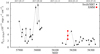 |
Fig. 1. Long-term X-ray light curve of Fermi J1544–0639 (unabsorbed 0.3–10 keV flux). The black dots denote the Swift/XRT exposures, while the large red dots denote the XMM-Newton observation, separated into three intervals (see Fig. 3 and Sect. 3.2). |
The paper is organized as follows. In Sect. 2 we describe the XMM-Newton observation and data reduction. In Sect. 3 we discuss the spectral analysis. In Sect. 4 we discuss the results, and in Sect. 5 we summarize the conclusions.
2. Observation and data reduction
Fermi J1544–0639 was observed by XMM-Newton on February 21, 2018 with a net exposure of 56 ks (Obs. Id. 0811213301). The data were processed using the XMM-Newton Science Analysis System (SAS v17.0).
The optical monitor (OM; Mason et al. 2001) photometric filters were operated in the Science User Defined image/fast mode. The OM images were taken with all of the six filters (V, B, U, UVW1, UVM2, and UVW2), with a continuous exposure time of 4.4 ks for each image (one image for V and U, two images for B and UVW1, three images for UVM2 and UVW2). The OM data were processed with the standard SAS pipelines OMICHAIN and OMFCHAIN, and prepared for the spectral analysis using the SAS task OM2PHA. We performed the spectral analysis on the stacked exposures for each filter, since no strong and significant temporal variability is observed from the inspection of the OM light curves (plotted in Fig. 2). The largest variation, namely 10% in count rate, occurs between the two UVW1 exposures.
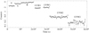 |
Fig. 2. XMM-Newton/OM light curves of Fermi J1544–0639 for each filter. Bins of 400 s are used. |
The EPIC instruments, pn and MOS (Strüder et al. 2001; Turner et al. 2001), were operating in the Large Window mode, with the thin filter applied. Because of the much higher effective area of the pn detector compared with MOS, throughout the paper we discuss results obtained from pn data. However, we checked that the spectral parameters were consistent among MOS and pn, albeit with larger uncertainties in MOS. Source extraction radii and screening for high-background intervals were determined through an iterative process that maximizes the signal-to-noise ratio (Piconcelli et al. 2004). The background was extracted from a circular region with a radius of 50 arcsec, while the source extraction radii were allowed to be in the range 20–40 arcsec; the best extraction radius was found to be 40 arcsec. The light curves were corrected and background-subtracted using the SAS task EPICLCORR. The EPIC-pn spectra were grouped such that each spectral bin contained at least 30 counts, and did not oversample the instrumental energy resolution by a factor greater than 3. We obtained poor fits near 1.8 and 2.2 keV, namely the energies of the instrumental silicon and gold edges. For this reason, we excluded the 1.75–2.25 keV range from the fits. For the spectral analysis, we used the full pn band 0.3–10 keV.
In Fig. 3 we show the XMM-Newton/pn light curves in the 0.5–2 keV and 2–10 keV energy ranges with the hardness ratio, background subtracted and corrected using the standard SAS tool EPICLCCORR. We use time bins of 1 ks to have uncertainties of a few percentage points in each bin. The source is strongly variable, both in flux (up to a factor of 4 in the 2–10 keV count rate) and in spectral shape, with a clear “harder-when-brighter” trend. We plot the hardness-intensity diagram, namely the hardness ratio versus the 2–10 keV count rate, in Fig. 4. We calculated the fractional rms variability amplitude (Fvar; e.g. Vaughan et al. 2003) using the tool LCSTATS in XRONOS. For the 0.5–2 keV light curve and the 2–10 keV light curve we found an Fvar of 0.26 ± 0.02 and 0.49 ± 0.05, respectively. To perform a time-resolved spectral analysis, we split the total exposure into three intervals, labelled A (15 ks long), B (20 ks), and C (21 ks), on the basis of the hardness ratio. The mean 2–10 keV/0.5–2 keV hardness ratio for the intervals A, B, and C is 0.28, 0.20, and 0.17, respectively. The first interval (int. A) thus corresponds to the harder/brighter state, while the third (int. C) corresponds to the softer/fainter state. This choice allows us to explore different spectral states with comparable statistics. We list the observed number of EPIC-pn counts for each interval in Table 1, together with the net exposure.
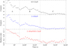 |
Fig. 3. XMM-Newton/pn light curve of Fermi J1544–0639. Bins of 1 ks are used. Top panel: count rate light curve in the 0.5–2 keV range. Middle panel: count rate light curve in the 2–10 keV range. Bottom panel: hardness ratio (2–10/0.5–2 keV) light curve. The vertical dashed lines separate the three intervals (A, B, C) defined for the spectral analysis. The solid horizontal lines correspond to the average hardness ratio for each interval. |
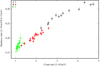 |
Fig. 4. Hardness ratio plotted against the 2–10 keV count rate for the three intervals A (black), B (red), and C (green). Time bins of 1 ks are used. |
Net exposure and number of pn counts in the 0.3–10 keV band for the different intervals.
3. Spectral analysis
We performed the spectral analysis with the XSPEC 12.10 package (Arnaud 1996). The binned pn spectra and the OM photometric data were analysed using the χ2 minimization technique. All errors are quoted at the 90% confidence level (Δχ2 = 2.71) for one interesting parameter. In the fits we always included neutral absorption (PHABS model in XSPEC) from Galactic hydrogen with column density NH = 8.7 × 1020 cm−2 (Kalberla et al. 2005). We assumed the element abundances of Anders & Grevesse (1989) and the photoelectric absorption cross sections of Verner et al. (1996).
3.1. Time-averaged spectrum
First, we fitted the average pn spectrum integrated over the full exposure. As a first step, we fitted the pn spectrum above 3 keV with a simple power law. Extrapolating this best-fitting power law to lower energies, we note a clear spectral break with a significant flattening below 2 keV (Fig. 5).
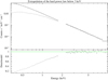 |
Fig. 5. Upper panel: time-averaged XMM-Newton/pn spectrum of Fermi J1544–0639. The power law that best fits the data in the 3–10 keV band is shown as a continuous curve. Lower panel: ratio of the observed spectrum (0.3–10 keV) to best-fit 3–10 keV power law. The data were binned for plotting purposes. |
Then we fitted the spectrum with a broken power law (BPL), characterized by the break energy Eb and by the photon indices Γ1 below the break and Γ2 above the break. We found a poor fit, with χ2/d.o.f. = 1030/155 and significant residuals with a bumpy shape below 2 keV (Fig. 6, upper panel). To account for this “soft excess”, we tried to include a further absorption component with ZPHABS in XSPEC. We first assumed a zero redshift, corresponding to an excess of Galactic absorption, finding a poor fit (χ2/d.o.f. = 492/154). Next, we assumed the redshift of the source, finding again a poor fit (χ2/d.o.f. = 360/154). Then, we removed the absorber and we included a blackbody with a free temperature kTBB. We found a much better fit (χ2/d.o.f. = 193/153, i.e. Δχ2/Δd.o.f. = −837/−2) and kTBB ≃ 0.2 keV, but still with significant positive residuals around 0.6 keV (Fig. 6, middle panel). The best-fitting parameters are listed in Table 2.
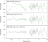 |
Fig. 6. Residuals of the fits of the time-averaged pn spectrum in the 0.3–10 keV band with the BPL model (Sect. 3.1). Top panel: simple broken power law. Middle panel: broken power law plus blackbody. Bottom panel: broken power law plus blackbody and a Gaussian line at 0.7 keV rest-frame. The data were binned for plotting purposes. |
To account for the residuals at 0.6 keV, we first included an ionized absorber (ZXIPCF in XSPEC) with free covering fraction, column density, and ionization parameter. We found a better fit (χ2/d.o.f. = 157/150, i.e. Δχ2/Δd.o.f. = −46/−3), whose parameters are listed in Table 2. However, we still found some positive residuals at 0.6 keV. We thus included a narrow Gaussian emission line, finding a better fit; in this case, the absorption component is not needed and its covering fraction is pegged at zero. We thus removed the ionized absorber, finally obtaining χ2/d.o.f. = 142/151, i.e. Δχ2/Δd.o.f. = −15/+1 (Fig. 6, lower panel; the probability of chance improvement is 9 × 10⁻¹¹ from an F-test). The best-fitting parameters are given in Table 2. The line is found to have a rest-frame energy of  keV and, if physical, might be interpreted as a blend of the two 2p−3s lines of Fe XVII at 17.05−17.10 Å. In Sect. 3.2 we show that neither the soft excess nor the emission line are artefacts of variability.
Furthermore, we checked whether the line detection is affected by the assumed elemental abundances. For this test, we switched to the abundances of Asplund et al. (2009). We obtained a slightly worse fit with χ2/d.o.f. = 155/151 and residuals at 0.3–0.4 keV suggestive of a slight excess of absorption. We thus added a further PHABS component, finding a good fit and no need for the Gaussian emission line. Removing the line, we obtained χ2/d.o.f. = 144/152 and a column density of (2.1 ± 0.8)×1020 cm−2 in excess of the value of Kalberla et al. (2005). The other parameters of the fit are not strongly altered by the different abundances. Analogous results were found assuming the abundances of Lodders (2003). Therefore, we cannot exclude that the residuals at 0.6 keV (observer-frame) are due to an imperfect modelling of Galactic absorption. However, in the subsequent analysis we decide to assume the Anders & Grevesse (1989) abundances and modelled the residuals with a phenomenological Gaussian emission line, which is more consistent with the RGS data (see Appendix A). Finally, to test whether the putative emission line is consistent with an origin from the hot interstellar medium of the host galaxy, we replaced it with the thermal plasma model APEC, v3.0.9 (Smith et al. 2001). We obtained a good fit (χ2/d.o.f. = 149/151). In general, the element abundances are consistent with being solar. However, some positive residuals near 0.4 keV (rest-frame) could indicate an enhanced emission from N VI. Leaving the nitrogen abundance (relative to solar) AN free, we obtain χ2/d.o.f. = 141/150 (Δχ2/Δd.o.f. = −8/−1) and  times solar. The other parameters are given in Table 2. We note that the APEC component alone is not able to reproduce the soft excess; indeed, removing the blackbody results in a poor fit (χ2/d.o.f. = 355/152).
The intrinsic (i.e. unabsorbed) flux in the 0.3–10 keV band is (3.61 ± 0.01)×10−11 ergs s−1 cm−2, not far from the average of 4.7 × 10⁻¹¹ ergs s−1 cm−2 recorded by Swift/XRT in summer 2017 (Sokolovsky et al. 2017, see also Fig. 1).
To try to further characterize the curvature of the X-ray spectrum, we fitted the data with a log-parabolic spectral law. We obtained similar results concerning the presence of the soft excess, although the final fit is statistically worse than the BPL best fit. This analysis is discussed in detail in Appendix B.
Next, we fitted the time-averaged pn spectrum jointly with the optical/UV data from the OM. In these fits we included interstellar extinction (REDDEN model in XSPEC) with E(B − V)=0.15 (Schlegel et al. 1998). We also included the host galaxy contribution, employing a template spectrum of an elliptical galaxy (Kinney et al. 1996) and leaving its normalization free to vary.
We started from the BPL best fit of the pn spectrum including the blackbody and Gaussian line. This model yields a poor fit in the OM band (χ2/d.o.f. = 221/156). Then we tested for the presence of a further emission component in the optical/UV band, which we modelled with a multicolour disc blackbody (DISKBB in XSPEC: Mitsuda et al. 1984; Makishima et al. 1986). We found an improved but still unacceptable fit with χ2/d.o.f. = 189/154. This is likely due to the fact that the primary X-ray power law cannot extend down to the optical/UV band. Therefore, we tested a different model allowing for a second spectral break at low energies. We thus replaced the broken power law with a double-broken power law (2-BPL). The 2-BPL is characterized by three different photon indices (Γ0, Γ1, and Γ2) and by two different break energies (Eb, 1 and Eb, 2). First, we assumed a negligible optical/UV contribution from the X-ray power law by freezing the low-energy break Eb, 1 at 0.1 keV. We obtained a good fit with χ2/d.o.f. = 158/153 (Δχ2/Δd.o.f. = −31/−1). Then we left the low-energy break of the 2-BPL free. We obtained a further improvement and no need for the DISKBB component, whose normalization became consistent with zero. We thus removed the DISKBB and obtained χ2/d.o.f. = 151/154 (Δχ2/Δd.o.f. = −7/+1), with a low-energy break at ∼5 eV. In Fig. 7 we show the data with residuals and best-fitting model, while the best-fitting parameters are given in Table 3.
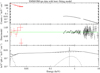 |
Fig. 7. Time-averaged XMM-Newton spectrum with best-fitting 2-BPL model (Sect. 3.1). Upper panel: OM (red) and pn (black) data with folded model. Middle panel: data-to-model ratio. Lower panel: best-fitting model E2f(E), without Galactic absorption and reddening, including the double-broken power law (dashed line) plus the blackbody, the Gaussian line, and the host galaxy (dotted lines). The data were binned for plotting purposes. |
Extrapolating the best-fitting model to the boundaries of the 0.001–10 keV band, we find an intrinsic luminosity of (6.22 ± 0.08)×1045 ergs s−1 cm−2.
3.2. Time-resolved spectral analysis of pn data
Having obtained a characterization of the time-integrated spectrum, we moved to the analysis of the pn spectra of the three intervals A, B, and C separately. Since our goal was to study the spectral variability in the X-ray band, we did not include the OM data for simplicity.
As in Sect. 3.1, we started by fitting the three pn spectra with the BPL model. We left the photon indices (Γ1 and Γ2), the break energy (Eb), and the normalization of the BPL free to vary among the different intervals. We found a poor fit, with χ2/d.o.f. = 1347/422 and significant residuals with a bumpy shape below 2 keV (see Fig. 8). To account for these residuals, we included a blackbody, leaving its normalization free to vary among the three spectra; the temperature kTBB was free but tied among the three intervals, with no detectable improvement by allowing it to change. We found a much better fit (χ2/d.o.f. = 490/418, i.e. Δχ2/Δd.o.f. = −857/−4), still with significant residuals around 0.6 keV (Fig. 8). A further improvement was found by adding a constant, narrow Gaussian emission line (χ2/d.o.f. = 441/416, i.e. Δχ2/Δd.o.f. = −49/−2; the probability of chance improvement is 3 × 10⁻¹⁰ from an F-test). The best-fitting parameters are listed in Table 4, while in Fig. 9 we show the contour plots of the two photon indices for the three intervals. The difference ΔΓ = Γ2 − Γ1 is around 0.6–0.7. We also tested an absorption scenario to explain the residuals in the soft X-ray band. We thus removed the Gaussian line and included an ionized absorber (ZXIPCF in XSPEC). The covering fraction, column density, and ionization parameter were tied among the intervals. We found a worse fit with χ2/d.o.f. = 454/415, i.e. Δχ2 = +13/−1, and no statistical improvement by allowing the absorber parameters to change among the intervals. Finally, we included an APEC component instead of the single line, finding χ2/d.o.f. = 444/415 and a nitrogen abundance  relative to solar.
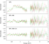 |
Fig. 8. Residuals of the fits of the three pn spectra in the 0.3–10 keV band with the BPL model (Sect. 3.2), for interval A (black), B (red), and C (green). Upper panel: simple broken power law. Middle panel: broken power law plus blackbody. Lower panel: broken power law plus blackbody and Gaussian line. The data were binned for plotting purposes. |
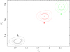 |
Fig. 9. Contour plots of the hard photon index Γ2 vs. the soft photon index Γ1 of the BPL model for interval A (black), B (red), and C (green). Solid, dashed, and dotted lines correspond to 68%, 90% and 99% confidence levels, respectively. |
4. Discussion
The X-ray properties of Fermi J1544–0639, as observed by XMM-Newton, are consistent overall with the identification of this object as a flaring radio-weak BL Lac (Bruni et al. 2018).
The source exhibits a strong X-ray variability during the XMM-Newton exposure, both in flux (Fvar ≃ 49% in the 2–10 keV band) and spectral shape, on timescales of ∼10 ks. The X-ray spectrum is clearly harder when the source is brighter, a behaviour typical of high-energy peaked BL Lacs (Pian 2002; Brinkmann et al. 2003; Krawczynski et al. 2004; Ravasio et al. 2004; Gliozzi et al. 2006; Zhang et al. 2006). In the synchrotron or inverse Compton scenario, this variability behaviour is generally understood in terms of a competition between acceleration and cooling processes (e.g. Tashiro et al. 1995; Kirk et al. 1998): since higher energy electrons cool faster, the spectrum steepens when the injection rate decreases. The mean X-ray luminosity νLν|1 keV is 1 × 1045 ergs s−1, a typical value for BL Lacs (e.g. Donato et al. 2001). We note that the XMM-Newton observation corresponds to an intermediate flux state of the source as recorded by the Swift/XRT monitoring, which will be discussed in a forthcoming work. The latest XRT exposures (up to July 2018) show that the source was still active, albeit in a lower flux state (Fig. 1).
The X-ray spectrum is nicely described by a broken power law; the spectral break occurs at around 2.7 keV and is consistent with being constant, regardless of the flux/spectral variations. The change in photon index is 0.6–0.7 (0.60 ± 0.03 on average), i.e. not far from the theoretical value of 0.5 expected in the presence of a radiative cooling break, either due to synchrotron or to inverse Compton in the Thomson limit (Kardashev 1962; Georganopoulos et al. 2001). Synchrotron cooling is expected to produce a break at an energy of
 (1)
(1)
where tesc is the escape time from the acceleration zone (see also Ponti et al. 2017). Assuming a magnetic field of 0.32 G, as derived from the SED modelling in Bruni et al. (2018), we can estimate tesc = 2 ks. In the hypothesis that the acceleration is due to Bohm-type diffusion (e.g. Stawarz & Ostrowski 2002), the escape time is related to the size D of the acceleration region as
 (2)
(2)
where η is a numerical factor and rg is the gyration radius. If η = 1 (Bohm limit),
 (3)
(3)
and we obtain D ∼ 109 cm. This spatial scale is much smaller than that required by causal connection, namely ctesc ≃ 6 × 1013 cm (see also Tammi & Duffy 2009). Moreover, D is only 10−5 in units of the Schwarzschild radius. The synchrotron cooling scenario thus appears unlikely to explain the observed spectral break. The radiative cooling could instead be dominated by Comptonization of external radiation fields, in particular from the BLR. When the cooling is dominated by inverse Compton of BLR photons, the spectral break can be evaluated as (Sikora et al. 2009)
 (4)
(4)
where Γ is the bulk Lorentz factor. Assuming a break energy of 2.66 keV (from the fit of the average spectrum), we obtain Γ = 16.3, in perfect agreement with the value estimated by Bruni et al. (2018). Since the break energy is consistent with being constant during the observation, we can infer that the bulk Lorentz factor is also consistent with being constant on a 50 ks timescale.
In addition to the primary continuum, a bumpy excess is found in the soft X-ray band. Intrinsic absorption is not able to reproduce this component, which phenomenologically is nicely described by a blackbody with a temperature of 0.22 keV. Its average 0.5–2 keV flux is 5 × 10⁻¹² ergs s−1 cm−2, corresponding to ∼20% of the flux of the primary power law in the same band. Moreover, the flux is found to decrease by ∼40% during the softer/fainter state, although there is no clear trend with the primary flux. We can interpret this soft emission component as being due to bulk Comptonization of low-energy photons in the jet. This process, first proposed by Begelman et al. (1987), consists in inverse Compton scattering of optical/UV diffuse radiation by cold electrons moving with a relativistic bulk velocity (see also Sikora et al. 1994). As later noted by Celotti et al. (2007), a bulk Comptonization component could explain the flattening in soft X-rays seen in the spectra of some sources, like the high-redshift blazar GB 1428+4217 (see also Worsley et al. 2004). In general, however, this feature can be difficult to observe because it can be transient and/or masked by the primary continuum (Celotti et al. 2007) or even absent if all the jet electrons are highly relativistic (Sikora et al. 2009).
So far, evidence of bulk Comptonization has been found in a handful of powerful sources like 4C 04.42 (de Rosa et al. 2008), PKS 1510–089 (Kataoka et al. 2008), and 4C 25.05 (Kammoun et al. 2018), which belong to the class of flat-spectrum radio quasars. To our knowledge, Fermi J1544–0639 is the first BL Lac showing possible evidence of bulk Comptonization. This could be due to the relative weakness of the jet, which does not outshine the bulk Comptonization component (although it dominates the X-ray emission). Further X-ray observations of other radio-weak BL Lacs could thus prove valuable to search for signatures of bulk Comptonization. According to the analysis of Celotti et al. (2007), an excess in the soft X-rays indicates that the most likely source of soft photons is the BLR rather than the accretion disc. This is due to a geometrical reason, since BLR photons are mostly seen head-on, and thus they can reach the maximum blueshift, i.e. ∼Γ2, where Γ is the bulk Lorentz factor. Following Celotti et al. (2007), Γ can be estimated by approximating the BLR emission as a blackbody spectrum. The relation between the temperature of the blackbody-like Comptonized emission kTBB and the BLR temperature kTBLR is thus kTBB ≃ Γ2kTBLR. Assuming Γ = 16.3, we obtain the plausible value TBLR ∼ 104 K (e.g. Peterson 2006). In principle, the BLR is illuminated by both the disc and the jet (Ghisellini & Madau 1996). However, given the low luminosity of the disc estimated by Bruni et al. (2018), the dominant source of illumination is likely the jet itself. Finally, the BLR clouds may not be the only source of seed photons: significant contributions could come from the molecular torus and intracloud plasma (Celotti et al. 2007).
In the optical/UV band, we find evidence of a significant emission component in addition to the host galaxy. The broad-band (optical/UV to X-rays) spectrum is nicely described by a double-broken power law with a low-energy break at 5 eV; if due to the jet, it could indicate a double-broken power law shape for the underlying electron distribution. An alternative origin involving blackbody-like disc emission is statistically disfavoured and is not consistent with the multiwavelength SED discussed by Bruni et al. (2018). However, given all the uncertainties, we cannot rule out a significant contribution from the accretion disc or the BLR. Moreover, the bulk Compton spectrum of disc photons is expected to peak in the UV band (Celotti et al. 2007). In any case, we can compare the luminosity of the optical/UV emission with that of the soft X-ray excess to further assess the validity of the bulk Comptonization scenario. First, the luminosity of the double-broken power law in the 0.001–0.1 keV band is 2.8 × 1045 ergs s−1. We can assume that around 10% of this luminosity is reprocessed and re-emitted by the BLR (Ghisellini & Madau 1996). We thus obtain a luminosity of the same order of magnitude as that of the soft X-ray excess, which is plausible in the bulk Compton scenario (Celotti et al. 2007). The mean UV luminosity νLν at 1015 Hz is 2 × 1044 ergs s−1 and is in good agreement with the SED reported in Bruni et al. (2018). A detailed analysis of the optical properties of the source is beyond the scope of this paper and is deferred to a dedicated study of all the optical follow-up data.
Finally, the soft X-ray spectrum, both time-averaged and time-resolved, displays an emission line at 0.70 keV (rest-frame) that can be tentatively attributed to Fe XVII. This feature could be due to thermal emission from the hot interstellar medium of the host galaxy. This is often observed in giant, non-active elliptical galaxies with temperatures generally ranging from 0.5 to 1 keV (Matsumoto et al. 1997; Xu et al. 2002; Tamura et al. 2003; Werner et al. 2009; Ogorzalek et al. 2017). In the present case, we can estimate a temperature of 0.28 keV and an observed luminosity of in the 0.1–10 keV range  . This can be compared to the luminosity of the host galaxy as derived from the historical magnitude reported in the Two Micron All Sky Survey (2MASS; Skrutskie et al. 2006). The 2MASS H-band magnitude of 2MASX J15441967–0649156 is 14.3, yielding for the luminosity in the H band
  in units of solar luminosities in the same band. Both
  and
and  are within the ranges of observed values for early-type, non-active galaxies (Ellis & O’Sullivan 2006), although
  is relatively high. However, we cannot exclude that the emission line is an artefact of an imperfect modelling of Galactic absorption. This issue might deserve further investigations through deeper X-ray observations since the detection of a soft X-ray emission line would be a quite surprising result for a BL Lac, if confirmed.
Fermi J1544–0639 is clearly a very peculiar jetted source. On the one hand, the gamma-ray flare was not followed by any enhancement of the radio activity, at least on a timescale of a few months; this could be due either to an inefficient jet collimation or to a large distance between the radio and gamma-ray emitting regions (Bruni et al. 2018). On the other hand, a new, bright X-ray source became visible ∼10 days after the gamma-ray flare, and remained active for more than one year (May 2017–July 2018). With a 0.1–2.4 keV flux of 1.7 × 10⁻¹¹ ergs s−1 cm−2 during the XMM-Newton observation, this source is two orders of magnitude brighter than the limiting flux of the ROSAT all-sky survey (10−13 ergs s−1 cm−2; Boller et al. 2016). This would imply an X-ray flare of a factor larger than 100. However, we can set a more conservative upper limit of ∼5 × 10⁻¹³ ergs s−1 cm−2 taking into account the ROSAT exposure in the field of the source (Salvato et al. 2018). The observed flux of the soft excess in the same band is 2 × 10⁻¹² ergs s−1 cm−2, i.e. at least a factor of 4 brighter than the ROSAT limiting flux. On the other hand, the putative thermal emission from the host galaxy has a flux of 7 × 10⁻¹³ ergs s−1 cm−2, namely comparable with the ROSAT limiting flux. It is thus possible that this component was present (as expected if it were due to the host galaxy), but not detected with ROSAT.
The multiwavelength properties of Fermi J1544–0639 seen so far indicate that this source is a low-power, radio-weak BL Lac that underwent a major outburst leading to the ignition of strong X-ray activity. In its pre-flare state, Fermi J1544–0639 was only a weak radio source with no other signatures of jet activity. This might suggest that Fermi J1544–0639 could mostly stay in a quiescent state, and become active following a sporadic ejection event (see also Gal-Yam et al. 2002). Additional monitoring will be needed to follow the evolution of the source, which might show a progressive decline and/or new episodes of activity. This would be desirable also to better constrain the variability of the different spectral components, especially of the soft excess/bulk Comptonization feature. Further observations of this and other similar sources will be needed to determine the rate and power of flares in this kind of objects and their incidence among the overall population of blazars.
5. Summary
We reported on the first XMM-Newton observation of the gamma-ray transient Fermi J1544–0639. Our main findings can be summarized as follows:
-
The X-ray variability is strong and indicative of a harder-when-brighter behaviour, consistent with the BL Lac nature of this object;
-
The X-ray primary continuum is nicely described by a variable broken power law, likely due to synchrotron emission from the jet; the spectral break at ∼2.7 keV is consistent with external Compton cooling, possibly from BLR photons;
-
The soft X-ray spectrum shows a blackbody-like soft excess, whose flux is around 20% of that of the primary power law, consistent with bulk Comptonization of BLR/intracloud plasma photons along the jet;
-
The optical/UV to X-ray spectrum is nicely described by a double-broken power law, suggesting that the jet dominates the UV emission; however, a significant contribution from the disc and/or the BLR cannot be ruled out;
-
A soft X-ray emission line is detected at 0.7 keV, which can be tentatively attributed to thermal emission of the host galaxy.
The peculiar properties of Fermi J1544–0639 motivate further observations of this and other radio-weak BL Lacs, which will improve our understanding of this new class of objects and, more generally, of the physics of extragalactic jets.
Acknowledgments
We thank the referee for a helpful and constructive review that significantly improved the manuscript. We acknowledge financial support from ASI under contracts ASI/INAF 2013-025-R1 and I/037/12/0. This work is based on observations obtained with XMM-Newton, an ESA science mission with instruments and contributions directly funded by ESA Member States and NASA.
References
- Anders, E., & Grevesse, N. 1989, Geochim. Cosmochim. Acta, 53, 197 [Google Scholar]
- Arnaud, K. A. 1996, in Astronomical Data Analysis Software and Systems V, eds. G. H. Jacoby, & J. Barnes, ASP Conf. Ser., 101, 17 [NASA ADS] [Google Scholar]
- Asplund, M., Grevesse, N., Sauval, A. J., & Scott, P. 2009, ARA&A, 47, 481 [NASA ADS] [CrossRef] [Google Scholar]
- Begelman, M. C., Sikora, M., Giommi, P., et al. 1987, ApJ, 322, 650 [NASA ADS] [CrossRef] [Google Scholar]
- Blandford, R. D., & Rees, M. J. 1978, in BL Lac Objects, ed. A. M. Wolfe, 328 [Google Scholar]
- Boller, T., Freyberg, M. J., Trümper, J., et al. 2016, A&A, 588, A103 [NASA ADS] [CrossRef] [EDP Sciences] [Google Scholar]
- Brinkmann, W., Papadakis, I. E., den Herder, J. W. A., & Haberl, F. 2003, A&A, 402, 929 [NASA ADS] [CrossRef] [EDP Sciences] [Google Scholar]
- Bruni, G., Panessa, F., Ghisellini, G., et al. 2018, ApJ, 854, L23 [NASA ADS] [CrossRef] [Google Scholar]
- Cao, H.-M., Frey, S., Gabányi, K. É., et al. 2019, MNRAS, 482, L34 [NASA ADS] [CrossRef] [Google Scholar]
- Cash, W. 1979, ApJ, 228, 939 [NASA ADS] [CrossRef] [Google Scholar]
- Cavaliere, A., & D’Elia, V. 2002, ApJ, 571, 226 [NASA ADS] [CrossRef] [Google Scholar]
- Celotti, A., Ghisellini, G., & Fabian, A. C. 2007, MNRAS, 375, 417 [NASA ADS] [CrossRef] [Google Scholar]
- Chornock, R., & Margutti, R. 2017, ATel, 10491 [Google Scholar]
- Ciprini, S., Cheung, C. C., Kocevski, D., et al. 2017, ATel, 10482 [Google Scholar]
- Condon, J. J., Cotton, W. D., Greisen, E. W., et al. 1998, AJ, 115, 1693 [NASA ADS] [CrossRef] [Google Scholar]
- de Rosa, A., Bassani, L., Ubertini, P., Malizia, A., & Dean, A. J. 2008, MNRAS, 388, L54 [NASA ADS] [CrossRef] [Google Scholar]
- den Herder, J. W., Brinkman, A. C., Kahn, S. M., et al. 2001, A&A, 365, L7 [NASA ADS] [CrossRef] [EDP Sciences] [Google Scholar]
- Diamond-Stanic, A. M., Fan, X., Brandt, W. N., et al. 2009, ApJ, 699, 782 [NASA ADS] [CrossRef] [Google Scholar]
- Donato, D., Ghisellini, G., Tagliaferri, G., & Fossati, G. 2001, A&A, 375, 739 [NASA ADS] [CrossRef] [EDP Sciences] [Google Scholar]
- Ellis, S. C., & O’Sullivan, E. 2006, MNRAS, 367, 627 [NASA ADS] [CrossRef] [Google Scholar]
- Fanaroff, B. L., & Riley, J. M. 1974, MNRAS, 167, 31P [Google Scholar]
- Fossati, G., Maraschi, L., Celotti, A., Comastri, A., & Ghisellini, G. 1998, MNRAS, 299, 433 [NASA ADS] [CrossRef] [Google Scholar]
- Foster, A. R., Ji, L., Smith, R. K., & Brickhouse, N. S. 2012, ApJ, 756, 128 [NASA ADS] [CrossRef] [Google Scholar]
- Gal-Yam, A., Ofek, E. O., Filippenko, A. V., Chornock, R., & Li, W. 2002, PASP, 114, 587 [NASA ADS] [CrossRef] [Google Scholar]
- Georganopoulos, M., Kirk, J. G., & Mastichiadis, A. 2001, ApJ, 561, 111 [NASA ADS] [CrossRef] [Google Scholar]
- Ghisellini, G., & Madau, P. 1996, MNRAS, 280, 67 [NASA ADS] [CrossRef] [Google Scholar]
- Ghisellini, G., & Tavecchio, F. 2008, MNRAS, 387, 1669 [NASA ADS] [CrossRef] [Google Scholar]
- Ghisellini, G., Padovani, P., Celotti, A., & Maraschi, L. 1993, ApJ, 407, 65 [Google Scholar]
- Ghisellini, G., Celotti, A., Fossati, G., Maraschi, L., & Comastri, A. 1998, MNRAS, 301, 451 [NASA ADS] [CrossRef] [Google Scholar]
- Ghisellini, G., Righi, C., Costamante, L., & Tavecchio, F. 2017, MNRAS, 469, 255 [NASA ADS] [CrossRef] [Google Scholar]
- Giommi, P., Padovani, P., Polenta, G., et al. 2012, MNRAS, 420, 2899 [NASA ADS] [CrossRef] [Google Scholar]
- Gliozzi, M., Sambruna, R. M., Jung, I., et al. 2006, ApJ, 646, 61 [NASA ADS] [CrossRef] [Google Scholar]
- Intema, H. T., Jagannathan, P., Mooley, K. P., & Frail, D. A. 2017, A&A, 598, A78 [NASA ADS] [CrossRef] [EDP Sciences] [Google Scholar]
- Kalberla, P. M. W., Burton, W. B., Hartmann, D., et al. 2005, A&A, 440, 775 [NASA ADS] [CrossRef] [EDP Sciences] [Google Scholar]
- Kammoun, E. S., Nardini, E., Risaliti, G., et al. 2018, MNRAS, 473, L89 [NASA ADS] [CrossRef] [Google Scholar]
- Kardashev, N. S. 1962, Soviet Ast., 6, 317 [Google Scholar]
- Kataoka, J., Madejski, G., Sikora, M., et al. 2008, ApJ, 672, 787 [NASA ADS] [CrossRef] [Google Scholar]
- Kinney, A. L., Calzetti, D., Bohlin, R. C., et al. 1996, ApJ, 467, 38 [NASA ADS] [CrossRef] [Google Scholar]
- Kirk, J. G., Rieger, F. M., & Mastichiadis, A. 1998, A&A, 333, 452 [NASA ADS] [Google Scholar]
- Kirsch, M. G. F., Altieri, B., Chen, B., et al. 2004, in UV and Gamma-Ray Space Telescope Systems, eds. G. Hasinger, & M. J. L. Turner, Proc. SPIE, 5488, 103 [NASA ADS] [CrossRef] [Google Scholar]
- Krawczynski, H., Hughes, S. B., Horan, D., et al. 2004, ApJ, 601, 151 [NASA ADS] [CrossRef] [Google Scholar]
- Lodders, K. 2003, ApJ, 591, 1220 [NASA ADS] [CrossRef] [Google Scholar]
- Makishima, K., Maejima, Y., Mitsuda, K., et al. 1986, ApJ, 308, 635 [NASA ADS] [CrossRef] [Google Scholar]
- Marchesini, E. J., Masetti, N., Chavushyan, V., et al. 2016, A&A, 596, A10 [NASA ADS] [CrossRef] [EDP Sciences] [Google Scholar]
- Marscher, A. 2016, Galaxies, 4, 37 [NASA ADS] [CrossRef] [Google Scholar]
- Masetti, N., Sbarufatti, B., Parisi, P., et al. 2013, A&A, 559, A58 [NASA ADS] [CrossRef] [EDP Sciences] [Google Scholar]
- Mason, K. O., Breeveld, A., Much, R., et al. 2001, A&A, 365, L36 [NASA ADS] [CrossRef] [EDP Sciences] [Google Scholar]
- Massaro, E., Perri, M., Giommi, P., & Nesci, R. 2004, A&A, 413, 489 [NASA ADS] [CrossRef] [EDP Sciences] [Google Scholar]
- Massaro, F., D’Abrusco, R., Ajello, M., Grindlay, J. E., & Smith, H. A. 2011, ApJ, 740, L48 [NASA ADS] [CrossRef] [Google Scholar]
- Massaro, F., Marchesini, E. J., D’Abrusco, R., et al. 2017, ApJ, 834, 113 [NASA ADS] [CrossRef] [Google Scholar]
- Matsumoto, H., Koyama, K., Awaki, H., et al. 1997, ApJ, 482, 133 [NASA ADS] [CrossRef] [Google Scholar]
- Mitsuda, K., Inoue, H., Koyama, K., et al. 1984, PASJ, 36, 741 [NASA ADS] [Google Scholar]
- Ogorzalek, A., Zhuravleva, I., Allen, S. W., et al. 2017, MNRAS, 472, 1659 [NASA ADS] [CrossRef] [Google Scholar]
- Padovani, P. 2017, Nat. Astron., 1, 0194 [NASA ADS] [CrossRef] [Google Scholar]
- Paggi, A., Massaro, F., D’Abrusco, R., et al. 2013, ApJS, 209, 9 [NASA ADS] [CrossRef] [Google Scholar]
- Paliya, V. S., Parker, M. L., Stalin, C. S., et al. 2015, ApJ, 803, 112 [NASA ADS] [CrossRef] [Google Scholar]
- Peterson, B. M. 2006, in Physics of Active Galactic Nuclei at all Scales, ed. D. Alloin (Berlin: Springer Verlag), Lecture Notes in Physics, 693, 77 [NASA ADS] [CrossRef] [Google Scholar]
- Pian, E. 2002, PASA, 19, 49 [NASA ADS] [CrossRef] [Google Scholar]
- Pian, E., Vacanti, G., Tagliaferri, G., et al. 1998, ApJ, 492, L17 [NASA ADS] [CrossRef] [Google Scholar]
- Pian, E., Foschini, L., Beckmann, V., et al. 2006, A&A, 449, L21 [NASA ADS] [CrossRef] [EDP Sciences] [Google Scholar]
- Piconcelli, E., Jimenez-Bailón, E., Guainazzi, M., et al. 2004, MNRAS, 351, 161 [NASA ADS] [CrossRef] [Google Scholar]
- Plotkin, R. M., Anderson, S. F., Brandt, W. N., et al. 2010, ApJ, 721, 562 [NASA ADS] [CrossRef] [Google Scholar]
- Ponti, G., George, E., Scaringi, S., et al. 2017, MNRAS, 468, 2447 [NASA ADS] [CrossRef] [Google Scholar]
- Ravasio, M., Tagliaferri, G., Ghisellini, G., & Tavecchio, F. 2004, A&A, 424, 841 [NASA ADS] [CrossRef] [EDP Sciences] [Google Scholar]
- Ricci, F., Massaro, F., Landoni, M., et al. 2015, AJ, 149, 160 [NASA ADS] [CrossRef] [Google Scholar]
- Salvato, M., Buchner, J., Budavári, T., et al. 2018, MNRAS, 473, 4937 [NASA ADS] [CrossRef] [Google Scholar]
- Schlegel, D. J., Finkbeiner, D. P., & Davis, M. 1998, ApJ, 500, 525 [NASA ADS] [CrossRef] [Google Scholar]
- Sikora, M., Begelman, M. C., & Rees, M. J. 1994, ApJ, 421, 153 [NASA ADS] [CrossRef] [Google Scholar]
- Sikora, M., Stawarz, Ł., Moderski, R., Nalewajko, K., & Madejski, G. M. 2009, ApJ, 704, 38 [NASA ADS] [CrossRef] [Google Scholar]
- Skrutskie, M. F., Cutri, R. M., Stiening, R., et al. 2006, AJ, 131, 1163 [NASA ADS] [CrossRef] [Google Scholar]
- Smith, R. K., Brickhouse, N. S., Liedahl, D. A., & Raymond, J. C. 2001, ApJ, 556, L91 [NASA ADS] [CrossRef] [Google Scholar]
- Sokolovsky, K., Cusano, F., Dominik, M., et al. 2017, ATel, 10642 [Google Scholar]
- Stawarz, Ł., & Ostrowski, M. 2002, ApJ, 578, 763 [NASA ADS] [CrossRef] [Google Scholar]
- Strüder, L., Briel, U., Dennerl, K., et al. 2001, A&A, 365, L18 [NASA ADS] [CrossRef] [EDP Sciences] [Google Scholar]
- Tammi, J., & Duffy, P. 2009, MNRAS, 393, 1063 [NASA ADS] [CrossRef] [Google Scholar]
- Tamura, T., Kaastra, J. S., Makishima, K., & Takahashi, I. 2003, A&A, 399, 497 [NASA ADS] [CrossRef] [EDP Sciences] [Google Scholar]
- Tashiro, M., Makishima, K., Ohashi, T., et al. 1995, PASJ, 47, 131 [NASA ADS] [Google Scholar]
- Tavecchio, F., & Ghisellini, G. 2008, MNRAS, 386, 945 [NASA ADS] [CrossRef] [Google Scholar]
- Terashima, Y., & Wilson, A. S. 2003, ApJ, 583, 145 [NASA ADS] [CrossRef] [Google Scholar]
- Tramacere, A., Massaro, F., & Cavaliere, A. 2007, A&A, 466, 521 [NASA ADS] [CrossRef] [EDP Sciences] [Google Scholar]
- Turner, M. J. L., Abbey, A., Arnaud, M., et al. 2001, A&A, 365, L27 [NASA ADS] [CrossRef] [EDP Sciences] [Google Scholar]
- Urry, C. M., & Padovani, P. 1995, PASP, 107, 803 [NASA ADS] [CrossRef] [Google Scholar]
- Vanden Berk, D. E., Lee, B. C., Wilhite, B. C., et al. 2002, ApJ, 576, 673 [NASA ADS] [CrossRef] [Google Scholar]
- Vaughan, S., Edelson, R., Warwick, R. S., & Uttley, P. 2003, MNRAS, 345, 1271 [NASA ADS] [CrossRef] [Google Scholar]
- Verner, D. A., Ferland, G. J., Korista, K. T., & Yakovlev, D. G. 1996, ApJ, 465, 487 [NASA ADS] [CrossRef] [Google Scholar]
- Voges, W., Aschenbach, B., Boller, T., et al. 1999, A&A, 349, 389 [NASA ADS] [Google Scholar]
- Werner, N., Zhuravleva, I., Churazov, E., et al. 2009, MNRAS, 398, 23 [NASA ADS] [CrossRef] [Google Scholar]
- Worsley, M. A., Fabian, A. C., Celotti, A., & Iwasawa, K. 2004, MNRAS, 350, L67 [NASA ADS] [CrossRef] [Google Scholar]
- Xu, H., Kahn, S. M., Peterson, J. R., et al. 2002, ApJ, 579, 600 [NASA ADS] [CrossRef] [Google Scholar]
- Zhang, Y. H., Treves, A., Maraschi, L., Bai, J. M., & Liu, F. K. 2006, ApJ, 637, 699 [NASA ADS] [CrossRef] [Google Scholar]
Appendix A: RGS spectrum
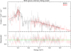 |
Fig. A.1. Upper panel: time-averaged RGS spectrum (0.4–1 keV) with best-fitting model. Lower panel: data-to-model ratio. The data were binned for plotting purposes. |
We analysed the data from the Reflection Grating Spectrometer (RGS; den Herder et al. 2001) with the main goal of further constraining the putative emission line at 0.6 keV seen in the pn spectrum. The RGS data were extracted using the standard SAS task RGSPROC. To obtain a good signal-to-noise ratio, we fitted the time-averaged spectra from the two detectors RGS1 and RGS2 in the 0.3–2 keV band. The spectra were not binned and were analysed using the C-statistic (Cash 1979). Starting with a simple power law, we found a quite poor fit with C/d.o.f. = 5870/5255. Prompted by the results of the pn data analysis of Sect. 3.1, we included a blackbody, finding an improved fit (C/d.o.f. = 5648/5253, i.e. ΔC/Δd.o.f. = −222/−2). We obtained a further improvement by adding a Gaussian emission line, with a free energy and intrinsic width (C/d.o.f. = 5633/5250, i.e. ΔC/Δd.o.f. = −15/−3). The RGS spectra with best-fitting model are plotted in Fig. A.1. The line energy was found to be 0.585 ± 0.007 keV, the intrinsic width  eV, and the flux
  in units of 10−4 photons cm−2 s−1. As such, the line has a flux consistent with that measured with the pn, while its energy is smaller by about 0.1 keV.
This mismatch could be due to cross-calibration issues between the two instruments (Kirsch et al. 2004). The line energy measured by RGS is close to, although not fully consistent with, that of the O VII Kα triplet (0.561–0.574 keV; Foster et al. 2012). This makes the identification of the atomic transition responsible for the emission line uncertain. We performed a similar analysis of the MOS time-averaged spectra in the 0.3–2 keV band, and we note that the line is found to have an energy of  keV, i.e. consistent with that found with the pn. Finally, as in Sect. 3.1, we switched to the elemental abundances of Asplund et al. (2009). We obtained a slightly worse fit with C/d.o.f. = 5640/5250 (ΔC = +7). Including a further PHABS component, we obtained C/d.o.f. = 5634/5249 and a column density of (4 ± 2)×1020 cm−2. The parameters of the Gaussian line are not significantly altered, thus indicating that the line detection in RGS is not affected by the assumptions on elemental abundances.
Appendix B: Testing the log-parabola
As an alternative to the BPL model discussed in Sect. 3, we fitted the pn data with a log-parabolic spectral law (LP) with νFν normalization (EPLOGPAR in XSPEC; Massaro et al. 2004; Tramacere et al. 2007). In this model, the spectral shape is determined by the curvature parameter β and by Ep, the peak energy in νFν.
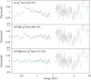 |
Fig. B.1. Residuals of the fit of the time-averaged pn spectrum in the 0.3–10 keV band with the LP model (Sect. 3.1). Top panel: simple log-parabola. Middle panel: log-parabola plus blackbody. Bottom panel: log-parabola plus blackbody and a Gaussian emission line at 0.7 keV. The data were binned for plotting purposes. |
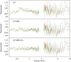 |
Fig. B.2. Residuals of the fits of the three pn spectra in the 0.3–10 keV band with the LP model. Upper panel: simple log-parabola. Middle panel: log-parabola plus blackbody. Lower panel: log-parabola plus blackbody and Gaussian line. The data were binned for plotting purposes. |
We started by fitting the time-averaged pn spectrum, as in Sect. 3.1. Fitting with only EPLOGPAR, we found an unacceptable fit with χ2/d.o.f. = 426/156. Including a blackbody, as in the BPL fit, we found a significant improvement (χ2/d.o.f. = 200/154, i.e. Δχ2/Δd.o.f. = −226/−2). Finally, including a narrow Gaussian line at 0.7 keV we found a further improvement (χ2/d.o.f. = 171/152, i.e. Δχ2/Δd.o.f. = −29/−2). However, the final LP fit is statistically worse than the BPL best fit, especially in the harder band (Δχ2/Δd.o.f. = +29/+1). The residuals for the different LP fits are shown in Fig. B.1.
Best-fitting parameters for the time-resolved pn spectra (LP model: EPLOGPAR+BBODY+ZGAUSS).
Then, we tested the LP model on the OM+pn data, as in Sect. 3.1. The LP model alone is not adequate to reproduce the broad-band spectrum, as even after re-fitting it yields χ2/d.o.f. = 629/151. We obtained a strong improvement by adding a DISKBB component; however, the fit is still relatively poor (χ2/d.o.f. = 167/149), mainly because of significant residuals above 2 keV (as in Fig. B.1).
Finally, we performed a time-resolved spectral analysis of the three intervals A, B, and C, as in Sect. 3.2. The curvature parameter of the LP and its peak energy, as well as the normalization, were left free to vary among the different intervals. Fitting with only EPLOGPAR, we found an unacceptable fit with χ2/d.o.f. = 702/425. Including a blackbody, we found a significant improvement (χ2/d.o.f. = 495/421, i.e. Δχ2/Δd.o.f. = −207/−4). Finally, including a narrow Gaussian line at 0.7 keV we found a further improvement (χ2/d.o.f. = 467/419, i.e. Δχ2/Δd.o.f. = −28/−2). Still, the fit is statistically worse than the BPL best fit (Δχ2/Δd.o.f. = +26/+3). The residuals for the different models are shown in Fig. B.2, while the best-fitting parameters are listed in Table B.1.
All Tables
Net exposure and number of pn counts in the 0.3–10 keV band for the different intervals.
Best-fitting parameters for the time-resolved pn spectra (LP model: EPLOGPAR+BBODY+ZGAUSS).
All Figures
|
Fig. 1. Long-term X-ray light curve of Fermi J1544–0639 (unabsorbed 0.3–10 keV flux). The black dots denote the Swift/XRT exposures, while the large red dots denote the XMM-Newton observation, separated into three intervals (see Fig. 3 and Sect. 3.2). |
| In the text | |
|
Fig. 2. XMM-Newton/OM light curves of Fermi J1544–0639 for each filter. Bins of 400 s are used. |
| In the text | |
|
Fig. 3. XMM-Newton/pn light curve of Fermi J1544–0639. Bins of 1 ks are used. Top panel: count rate light curve in the 0.5–2 keV range. Middle panel: count rate light curve in the 2–10 keV range. Bottom panel: hardness ratio (2–10/0.5–2 keV) light curve. The vertical dashed lines separate the three intervals (A, B, C) defined for the spectral analysis. The solid horizontal lines correspond to the average hardness ratio for each interval. |
| In the text | |
|
Fig. 4. Hardness ratio plotted against the 2–10 keV count rate for the three intervals A (black), B (red), and C (green). Time bins of 1 ks are used. |
| In the text | |
|
Fig. 5. Upper panel: time-averaged XMM-Newton/pn spectrum of Fermi J1544–0639. The power law that best fits the data in the 3–10 keV band is shown as a continuous curve. Lower panel: ratio of the observed spectrum (0.3–10 keV) to best-fit 3–10 keV power law. The data were binned for plotting purposes. |
| In the text | |
|
Fig. 6. Residuals of the fits of the time-averaged pn spectrum in the 0.3–10 keV band with the BPL model (Sect. 3.1). Top panel: simple broken power law. Middle panel: broken power law plus blackbody. Bottom panel: broken power law plus blackbody and a Gaussian line at 0.7 keV rest-frame. The data were binned for plotting purposes. |
| In the text | |
|
Fig. 7. Time-averaged XMM-Newton spectrum with best-fitting 2-BPL model (Sect. 3.1). Upper panel: OM (red) and pn (black) data with folded model. Middle panel: data-to-model ratio. Lower panel: best-fitting model E2f(E), without Galactic absorption and reddening, including the double-broken power law (dashed line) plus the blackbody, the Gaussian line, and the host galaxy (dotted lines). The data were binned for plotting purposes. |
| In the text | |
|
Fig. 8. Residuals of the fits of the three pn spectra in the 0.3–10 keV band with the BPL model (Sect. 3.2), for interval A (black), B (red), and C (green). Upper panel: simple broken power law. Middle panel: broken power law plus blackbody. Lower panel: broken power law plus blackbody and Gaussian line. The data were binned for plotting purposes. |
| In the text | |
|
Fig. 9. Contour plots of the hard photon index Γ2 vs. the soft photon index Γ1 of the BPL model for interval A (black), B (red), and C (green). Solid, dashed, and dotted lines correspond to 68%, 90% and 99% confidence levels, respectively. |
| In the text | |
|
Fig. A.1. Upper panel: time-averaged RGS spectrum (0.4–1 keV) with best-fitting model. Lower panel: data-to-model ratio. The data were binned for plotting purposes. |
| In the text | |
|
Fig. B.1. Residuals of the fit of the time-averaged pn spectrum in the 0.3–10 keV band with the LP model (Sect. 3.1). Top panel: simple log-parabola. Middle panel: log-parabola plus blackbody. Bottom panel: log-parabola plus blackbody and a Gaussian emission line at 0.7 keV. The data were binned for plotting purposes. |
| In the text | |
|
Fig. B.2. Residuals of the fits of the three pn spectra in the 0.3–10 keV band with the LP model. Upper panel: simple log-parabola. Middle panel: log-parabola plus blackbody. Lower panel: log-parabola plus blackbody and Gaussian line. The data were binned for plotting purposes. |
| In the text | |
Current usage metrics show cumulative count of Article Views (full-text article views including HTML views, PDF and ePub downloads, according to the available data) and Abstracts Views on Vision4Press platform.
Data correspond to usage on the plateform after 2015. The current usage metrics is available 48-96 hours after online publication and is updated daily on week days.
Initial download of the metrics may take a while.