| Issue |
A&A
Volume 622, February 2019
|
|
|---|---|---|
| Article Number | A140 | |
| Number of page(s) | 10 | |
| Section | Atomic, molecular, and nuclear data | |
| DOI | https://doi.org/10.1051/0004-6361/201834308 | |
| Published online | 11 February 2019 | |
Improved Ni II oscillator strengths from quasar absorption systems⋆
Sorbonne Université, CNRS, UMR 7095, Institut d’Astrophysique de Paris, 98 bis Bd Arago, 75014 Paris, France
e-mail: This email address is being protected from spambots. You need JavaScript enabled to view it.
Received:
24
September
2018
Accepted:
6
December
2018
Abstract
Aims. We wish to improve the accuracy of oscillator strength values for several Ni II UV transitions and measure for the first time the f-value of a few other weak transitions for which no laboratory nor astronomical measurement is presently available.
Methods. Four quasars displaying five damped Lyman α systems with relatively strong Ni II lines were selected. From the analysis of the excellent high resolution spectra available, we determined the relative f-value of Ni II transitions by comparing the strength of the corresponding absorption profiles. To quantify the latter, we used the apparent optical depth method for resolved features, equivalent width measurements for optically thin lines and line fitting with VPFIT. Absolute f-values were then derived by relating our determinations to the available laboratory measurements.
Results. Thanks to the good signal-to-noise ratio of the spectra and to the suitable properties of the absorption systems investigated, we are able to significantly improve the determination of the f-value for 13 Ni II transitions falling in the 1317–1804 Å interval. Our results are found to be consistent with other earlier determinations for ten of these transitions; our median relative accuracy for these f-values is 6.5%. For three weak transitions near 1502, 1773, and 1804 Å, which have not been detected previously in astronomical spectra, we can get a first measurement of their f-value.
Conclusions. Our work illustrates that, thanks to the redshift and the absence of variations of physical constants on cosmological scales, the analysis of absorption lines induced by remote gas in quasar spectra can nowadays provide valuable constraints on atomic data in the UV range.
Key words: atomic data / ultraviolet: ISM / quasars: absorption lines
Based on observations with VLT-UVES and Keck-HIRES.
© ESO 2019
 Open Access article, published by EDP Sciences, under the terms of the Creative Commons Attribution License (http://creativecommons.org/licenses/by/4.0), which permits unrestricted use, distribution, and reproduction in any medium, provided the original work is properly cited.
1. Introduction
Absorption line studies of interstellar or intergalactic gas seen in the spectra of bright sources such as stars, quasars, or gamma-ray bursts provide critical information on the physical conditions prevailing in the intervening material lying along these lines of sight. In order to get useful constraints on relative abundances, ionisation, excitation, temperature, or volume density for instance, a key step is to measure column densities (hereafter N) for the species detected. Once good signal-to-noise (S/N) spectra have been acquired, the analysis then directly relies on the knowledge of oscillator strength (f) values for the transitions involved. Generally, for the major transitions of interest, the accuracy of the atomic data is such that uncertainties in the column density determinations are set mainly by the quality of the spectra. However, for some species, commonly detected transitions still have poorly known f-values.
One of these species is Ni II, the dominant form of nickel in gas that is optically thick to radiation ionising hydrogen atoms. Ni II displays numerous resonant transitions in the UV covering a broad range of f-values, thus providing favourable conditions to get reliable column density estimates. The latter can then be used for instance to investigate the differential depletion of nickel onto dust grains (see e.g. Dessauges-Zavadsky et al. 2006) or nucleosynthetic effects. Prior to 1999, no laboratory measurements of Ni IIf-values were available and only theoretical calculations could be used (in his compilation, Morton 1991 refers to calculations performed by R. L. Kurucz). The latter cannot be accurate, especially for a species like Ni II (see Cassidy et al. 2016), which prompted Zsargó & Federman (1998) to get constraints directly from astrophysical data, namely GHRS/HST spectra of reddened stars. Soon after these astrophysical determinations, Fedchak & Lawler (1999) were able to establish an absolute scale and provide f-values for the three strong transitions at 1709, 1741, and 1751 Å. Fedchak et al. (2000) extended the previous laboratory work by performing measurements of relative f-values for four additional transitions beyond 1400 Å. For the strong 1317 and 1370 Å transitions, a rough estimate was provided by Ellison et al. (2001a) from the analysis of Ni II lines in a quasar damped Lyman α (DLA) system. These transitions were still poorly characterised, which led Jenkins & Tripp (2006) to use GHRS/HST spectra for a sample of reddened stars, resulting in a significant improvement of the determination of the relative 1317, 1370, 1454, and 1741 Å f-values. Finally, Dessauges-Zavadsky et al. (2006) obtained an independent measurement of the 1317 Å f-value (consistent with the one given by Jenkins & Tripp) from the analysis of five DLA systems. Despite all these studies, the accuracy of f-values for some major Ni II transitions (such as those at 1317 and 1370 Å) is still no better than about 10%. Further, some potentially useful transitions with f > 5 × 10⁻³ (e.g. those at 1502, 1773, and 1804 Å) listed in Morton (1991) have apparently never been observed in astrophysical spectra or measured at the laboratory, while they could help to get accurate estimates for N(Ni II). Indeed, in very large column density systems such as that studied by Balashev et al. (2017), lines associated with the strongest transitions may be saturated and weaker transitions could then provide a much more reliable determination.
In the course of a recent study devoted to partial covering effects in quasar absorption systems (Bergeron & Boissé 2017), we realised that for some bright quasars displaying strong DLA systems, the S/N of the available spectra is high enough to enable an improvement of relative f-values for several Ni II transitions. Since physical constants, at least α (the fine-structure constant) and μ (the proton-to-electron mass ratio), appear to suffer very little relative variations (upper limits of about 10−6 have been obtained; see e.g. Molaro et al. 2013) over cosmological times and distances, one can legitimately use observations of remote material to get constraints on the properties of local ions, atoms, or molecules.
Our purpose in this paper is thus to investigate in detail Ni II absorption line profiles in a few selected quasar absorption systems to get constraints on the oscillator strength of several transitions from this species. The content of this paper is organised as follows. In Sect. 2, we introduce the five quasar absorption systems considered as well as the methods used to analyse line profiles and infer Ni IIf-values. In Sect. 3, we describe the procedure adopted for each of the 13 Ni II transitions considered in our study (these are listed in Table 4) and the resulting f-values obtained. Next, we discuss the internal consistency of the obtained set of Ni IIf-values as well as the comparison with previously published values (Sect. 4). Finally, we conclude with some prospects concerning the use of distant quasar spectra to constrain f-values and summarise our main results (Sect. 5).
2. Quasar systems and analysis of absorption line profiles
2.1. Selection of quasar absorption systems
We selected four quasars displaying in total five strong DLA systems. We give details on the quasars in Table 1 while Table 2 provides information on the DLA absorption systems. All the absorption systems considered include relatively strong although apparently unsaturated Ni II absorption lines from several transitions covering the 1300–1810 Å wavelength interval. In three out of the five systems, Ni II absorption extends over an interval exceeding 50 km s−1, as can be seen in Fig. 1, where we show the velocity profiles of Ni IIλ1741, which is the third strongest Ni II transition. The presence of blends with features from other absorption systems can be assessed directly by comparing the profiles observed for all detected Ni II transitions; this will be illustrated in forthcoming figures. Good S/N and high resolution spectra from the UVES or HIRES databases are available for the four quasars; the spectral resolution of these data is of about five to six km s−1 full width at half maximum (hereafter FWHM). These data are all public; integration times and observing dates are listed in Table 1 for each quasar. Details about the UVES data can be found in Bergeron et al. (2004) and Molaro et al. (2013) while the HIRES spectra are described in Prochaska et al. (2007) and O’Meara et al. (2015). Generally, these bright targets involving remarkable absorption systems have been observed several times for various purposes. This allows us to further increase the S/N by combining all spectra, if needed to detect fainter transitions or to assess the reliability of the analysis by considering these data separately.
Quasar sample.
Quasar DLA absorption systems.
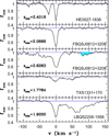 |
Fig. 1. Ni IIλ1741 absorption profile for the five systems considered in this study. The redshift of the strongest narrow absorption feature is indicated at the lower left corner of each panel and corresponds to vhelio = 0 km s−1. All features appearing in these profiles are from the Ni IIλ1741 transition except that shaded in the middle panel. |
We now give a brief overview of the main properties of each absorption system and indicate which Ni II transitions are detected. There are several reasons for the non-detection of transitions: i) the associated lines fall outside or in a gap of the spectrum, ii) they are blended with other features, and iii) the S/N is too poor at the expected wavelength.
– HE 0027–1836, zabs = 2.4018. The extensive UVES observations of high spectral resolution (FWHM = 5.0 km s−1) have essentially been used to constrain the variation of the proton-to-electron mass ratio, μ, on the basis of a detailed analysis of H2 absorptions from various rotational levels (Rahmani et al. 2013). This absorber was also studied by Balashev et al. (2015) to investigate the link between H2 and Cl I in cold neutral phases, as observed in the local interstellar medium.
The main velocity component at v = 0 km s−1 is unresolved. Another slightly broader and asymmetrical feature lies at v ≈ −20 km s−1 together with a very weak one at v ≈ −80 km s−1, which can be seen only for the strongest transitions. All the 13 transitions considered in this paper are detected in this system.
– FBQS J0812+3208, zabs = 2.0668. The column densities of many species are given by Prochaska et al. (2007). For this system as well as for that at zabs = 2.6263, the physical conditions in neutral gas have been derived from a study of C I fine-structure lines (Jorgenson et al. 2010).
There are two HIRES spectra of FBQS J0812+3208 both with similar spectral resolutions: an earlier spectrum (2002) with a higher S/N in the visible red (λ > 4600 Å) and a later one (2007) available in the KODIAQ database (O’Meara et al. 2015) with a higher S/N in the blue.
The absorption profile consists in a single narrow, slightly asymmetrical feature. All Ni II transitions dealt with in this paper are detected, except for λ1393 and λ1773.
– FBQS J0812+3208, zabs = 2.6263. Prochaska et al. (2003) determined the abundance pattern of the absorbing galaxy and found that the latter was enriched mainly by massive stars. From a curve of growth analysis of weak C I transitions, Jorgenson et al. (2009) concluded that the neutral gas is cold (T ≲ 115 K). These authors also measured a high column density of molecular hydrogen.
The available HIRES spectra are those already mentioned above. The profile consists in a strong, resolved (FWHM ≈ 16 km s−1) feature at v = 0 km s−1, accompanied by blue shallow absorption extending up to about −50 km s−1.
The unblended Ni II transitions detected are four of the five stronger ones (the λ1709 line profile is heavily blended with Mg IIλ2803 at zabs = 1.2112) together with λ1454, λ1467.7, λ1502, and λ1703.
– TXS 1331+170, zabs = 1.7763. A curve of growth analysis of the C I transitions has been used by Carswell et al. (2011) to derive the neutral gas temperature, T ≲ 220 K, which is low. The link between H2 and Cl I in cold neutral phases has also been investigated by Balashev et al. (2015).
Two spectra are available for TXS 1331+170: a UVES one (2011) with a resolution of 5.5 km s−1 (FWHM) and another obtained with HIRES (1994; at λ > 4220 Å) of lower spectral resolution.
The Ni II absorption profile comprises a resolved feature (FWHM ≈ 18 km s−1) at v = 0 km s−1 and extends at positive velocities up to v ≈ +70 km s−1. We detect only the five strongest Ni II transitions.
– LBQS 2206–1958, zabs = 1.9200. This is a well known metal-rich DLA system with accurate measurements of the abundances of several elements together with an investigation of the possible presence of dust (e.g. Bergeron & Petitjean 1991; Prochaska & Wolfe 1997).
There are three available spectra for this quasar: two UVES (2000 and 2011–2012; the latest has a FWHM of 6.0 km s−1 and is of higher S/N) and one of lower S/N obtained with HIRES in 1994 (see Table 1).
This system has fairly strong Ni II absorption lines including a strong partially resolved component at v = 0 km s−1 together with broad, fully resolved absorption extending up to v ≈ +150 km s−1. The unblended Ni II transitions detected are the five strongest and three weaker ones at 1703, 1773, and 1804 Å.
2.2. Apparent optical depth analysis
Three out of the five absorption systems presented above display Ni II line profiles extending over about 100 km s−1. A large fraction of these lines should then be fully resolved, as is generally observed for singly ionised species tracing H I regions (Wolfe et al. 2005). In this circumstance, it is appropriate to use the apparent optical depth (hereafter AOD) method (Savage & Sembach 1991), which should provide true opacity values along the velocity profile, τ(v), except where narrow components are present. Using this approach presents the great advantage of removing any arbitrariness associated with the choice of a particular set of discrete velocity components. The same is true for equivalent width measurements of optically thin lines (see Sect. 2.3). When blends or unresolved components are present, line fitting is needed (Sect. 2.4).
Let us consider two distinct transitions labelled i and j; since τ(v)∝λfN(v), the ratio of their f-values, fj/fi, is given by
 (1)
(1)
where τi(v) is obtained directly from In, i(v), the normalised absorption profile of transition i, through
 (2)
(2)
Thus, at velocities where the profile is fully resolved, the τj(v)/τi(v) ratio does not depend on velocity and should provide an unbiased estimate of the fj/fi ratio. The presence of a narrow unresolved component along the profile can be readily identified since the ratio defined by Eq. (1) is expected to display a distinct value in the corresponding velocity interval. In the same way, blending with another transition, as is often the case in quasar spectra including several absorption systems or if the line falls in the Lyα forest, can be easily recognised. The fj/fi ratio should then be derived from the average of (λi τj(v))/(λj τi(v)) values computed over the velocity interval unaffected by unresolved components or blends. The rms scatter about the mean directly provides an estimate of the uncertainty on the fj/fi value. The kind of result obtained for τi(v) profiles and for their ratio in the za = 1.9200 system towards LBQS 2206–1958 is illustrated by Fig. 2.
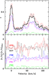 |
Fig. 2. Intervening Ni II absorption towards the quasar LBQS 2206–1958 at za ≈ 1.92. The opacity profiles for the 1317 (thin black line), 1370 (red), 1703 (green), 1709 (blue), 1741 (thick black), and 1751 Å (cyan) transitions are shown in the upper panel. The ratio of any given profile to the 1741 Å profile is shown in the lower panel. The ratios are better defined at velocities for which the opacity is large; they range from 0.125 (for 1703 Å) up to 1.43 (1370 Å), thus covering a dynamical range of 11.4. At vhelio = 0 km s−1, the redshift is za = 1.9200. |
Once a fj/fi ratio has been determined, the knowledge of the f-value for one of the two transitions is required to get the f-value of the other. In this work, we were able to perform several measurements involving three of the major Ni II transitions, at 1709, 1741, and 1751 Å, for which Fedchak & Lawler (1999) obtained absolute f-values from laboratory work. We chose to rely on these results by proceeding in two steps. First, we used our measured f-value ratios involving these three transitions to improve the accuracy of their absolute f-value (see Sect. 2.5 below). Next, we inferred f-values for other transitions from ratios involving one of the three 1709, 1741, and 1751 Å transitions. In this way, we get results that are related to those obtained by other teams (e.g. Fedchak et al. 2000; Jenkins & Tripp 2006) only through the absolute measurements of Fedchak & Lawler (1999), allowing us to check the consistency of the various determinations. We now describe the two other methods used in the following to analyse absorption profiles.
2.3. Equivalent widths of optically thin lines
For unresolved optically thin lines, it is appropriate to measure the equivalent width (hereafter W) and use the W ∝ λ2 f relationship to derive the oscillator strength of transitions with unknown f-values, by comparison with those of well- characterised transitions.
2.4. Line profile fitting with VPFIT
When line profiles from two distinct transitions are blended or if velocity components appear to be unresolved or partly resolved, the AOD method no longer allows us to recover the true line opacity. In these circumstances, profile fitting is an efficient method to model the absorption profile by introducing discrete Gaussian velocity components. Using VPFIT10.21 we determined the column densities, N, and Doppler parameters, b, associated with each component. In this work, we preferred not to derive f-values from line fitting to avoid any bias due to the choice of velocity components. Thus, we shall use line fitting with VPFIT only to verify that acceptable fits can be obtained for all detected Ni II absorption lines when the f-values derived from the two methods described above are adopted.
2.5. From relative to absolute f-values
Fedchak & Lawler (1999) measured absolute f-values with a relative accuracy of about 10%. The ratio of two f-values is then known with an accuracy of about 14%. If independent data, like those considered in this paper, provide significantly better constraints on these ratios, it should be possible to use this additional information to get improved absolute f-values.
We now describe how one can do so by considering two quantities, say A and B, for which the following measurements are available: A = A0 ± σA, B = B0 ± σB and R = A/B = R0 ± σR. In principle, the joint probability distribution for (A, B) should be considered, taking into account the known constraint on R = A/B and next, values of A and B maximising this distribution should be searched for. A more straightforward and intuitive approach can be used. Assuming that the three measurements are independent, it is possible to get a second estimate for A from B0 and  , the uncertainty of which is
 (3)
(3)
The values A0 and  are independent estimates of A, which can be combined in the optimal way using 1/σ2 weighting. We thus get an “improved” estimate for A:
 (4)
(4)
with an uncertainty,  , given by
 (5)
(5)
We can proceed similarly to get  and the improved estimate of B,
  . Obviously,
  and
and  and
and  and
and  are no longer statistically independent. It can be verified easily that if the relative accuracy on R is much better than that on A and B, the above procedure returns a value for
  significantly lower than σA/A0. Further, in the σR → 0 limit, we get
  , as expected. We could check that, in the limit of small relative uncertainties on f-values or on their ratio, which are of the order of 10% or less, this simplified procedure provides results that are similar to those obtained from the rigorous approach involving the (A, B) joint probability distribution.
3. Results for f-values
We first consider the three “primary” 1709, 1741, and 1751 Å transitions for which Fedchak & Lawler (1999) could obtain absolute f-values from laboratory experiments.
3.1. Transitions at 1709, 1741, and 1751 Å
All ratios can be computed from the broad profiles in the LBQS 2206–1958 zabs = 1.9200 and TXS 1331+170 zabs = 1.7764 systems. In the FBQS J0812+3208 zabs = 2.6263, the 1709 Å transition is blended with another feature, thus only the f(1751)/f(1741) ratio can be obtained. In Table 3, we give the values provided by each system for f(1709)/f(1741), f(1751)/f(1741), and f(1751)/f(1709). Given the 1σ errors, results obtained for each ratio from various absorption systems are mutually consistent; we thus compute their weighted average over the two or three systems considered.
Ratios of f-values for the 1709, 1741, and 1751 Å transitions.
Combining the above ratios with the absolute f-values of Fedchak & Lawler (1999) as explained in Sect. 2.5 (the extension of the method to three quantities and two ratios is straightforward), we get the following values:
-
f(1709) = 0.0318 ± 0.0018,
-
f(1741) = 0.0432 ± 0.0025,
-
f(1751) = 0.0280 ± 0.0015.
For other Ni II transitions, it is possible to get their f-value from the opacity ratio involving either of these three primary transitions; we can select the one providing in the end the f-value with the minimum uncertainty.
3.2. Ni II transitions with previous available measurements
Let us first discuss the other Ni II transitions for which measurements have already been performed, either at the laboratory (by Fedchak et al. 2000) or in astronomical spectra (by Zsargó & Federman 1998; Jenkins & Tripp 2006). In the following, we indicate for each of these transitions, which system(s) provides the most accurate determination and the method adopted to derive the f-value. We also mention the other systems that can be used to test the reliability of this value. Figures illustrating the quality of the corresponding fits are given in Sect. 4.
– λ = 1317.22 Å. The best constraints are derived using the AOD method for the FBQS J0812+3208 (zabs = 2.6263) system which provides a well-defined value for the f(1317)/f(1751) ratio f(1317)/f(1751) = 2.132 ± 0.068, from which we get f(1317) = 0.0596 ± 0.0037. All other four systems allow us to test this value.
– λ = 1370.13 Å. We proceed as with the previous 1317 Å transition and obtain f(1370)/f(1751) = 2.200 ± 0.052, implying f(1370) = 0.0616 ± 0.0036. The f(1317)/f(1370) ratio can also be derived from a direct comparison of the two 1317 and 1370 Å line profiles, which provides f(1317)/f(1370) = 0.972 ± 0.012. Again, all other systems can be used as a check.
– λ = 1393.32 Å. The line profile of this transition is seen (nearly) unblended only in the HE 0027–1836 system at zabs = 2.4018. The two main velocity components appear on the blue end of the broad Si IVλ1393 profile (see Sect. 4.1.1). Given the small opacity involved, we can use the Si IVλ1402 profile to define the local continuum appropriate for these two Ni II lines and estimate f(1393) from the comparison of the equivalent widths of the optically thin Ni IIλ1393 and Ni IIλ1703 lines. Averaging over the two velocity components, we get f(1393)/f(1703) = 2.32 ± 0.14, which results in f(1393) = 0.0125 ± 0.0012.
– λ = 1454.84 Å. The best constraints are derived from the main component of the FBQS J0812+3208, zabs = 2.6263 system. Using the AOD method, we get f(1454)/f(1741) = 0.510 ± 0.019, implying f(1454) = 0.0220 ± 0.0015. The zabs = 2.0668 system in FBQS J0812+3208 together with that at zabs = 2.4018 in HE 0027–1836 allow us to check this value.
– λ = 1467.26 Å and λ = 1467.76 Å. The 1467.7 Å line is seen in the resolved profile of both systems in FBQS J0812+3208 (at zabs = 2.6263) and LBQS 2206–1958 (zabs = 1.9200); but given the small opacity and low S/N, the continuum cannot be defined accurately. Better constraints are provided by the narrow zabs = 2.0668 system in FBQS J0812+3208, in which both lines are detected. Equivalent width measurements of the 1467.2, 1467.7, and 1703 Å Ni II lines yield f(1467.2)/f(1467.7) = 0.595 ± 0.086 together with f(1467.7)/f(1703) = 1.25 ± 0.19, resulting in f(1467.2) = 0.0040 ± 0.0009 and f(1467.7) = 0.0067 ± 0.0011. The system in HE 0027-1836 can be used to test these results, as well as the one at zabs = 2.6263 in FBQS J0812+3208 for λ1467.7.
– λ = 1703.41 Å. For this weak transition, the S/N is good enough and the continuum is sufficiently well defined such that the AOD method can be used for both systems in FBQS J0812+3208 (at zabs = 2.6263) and LBQS 2206–1958 (zabs = 1.9200). The combined value for the f(1703)/f(1741) ratio is f(1703)/f(1741) = 0.1258 ± 0.0056, implying f(1703) = 0.0054 ± 0.0004. Two other systems can be used as a test: the system in HE 0027–1836 and that in FBQS J0812+3208 at zabs = 2.6263.
3.3. Ni II transitions without previous measurements
To our knowledge, the three Ni II resonance transitions near 1502, 1773, and 1804 Å, listed in Morton (1991) with theoretical f-values of 0.0133, 0.0062, and 0.0072, respectively, have never been detected in astronomical spectra or investigated at the laboratory.
– λ = 1502.15 Å. The FBQS J0812+3208, zabs = 2.0668 system provides the best measurement for the f-value of this weak transition. Comparing the equivalent width to that of the Ni IIλ1703 feature, we get f(1502)/f(1703) = 1.42 ± 0.30 and then f(1502) = 0.0077 ± 0.0013. The two systems in HE 0027–1836 and FBQS J0812+3208 (zabs = 2.6263) provide a test for this value.
– λ = 1773.95 Å. This transition is clearly detected in the LBQS 2206–1958 zabs = 1.9200 system, even in the broad part of the profile. However, the latter would be difficult to exploit owing to the uncertainty in the placement of the continuum. Thus, we prefer to restrict our analysis to the narrow component at v ≈ 0 km s−1. From the ratio of its equivalent width to that of the 1703 Å transition (both features are clearly optically thin), we derive f(1773)/f(1703) = 0.774 ± 0.086, resulting in f(1773) = 0.0042 ± 0.0006. The system in HE 0027-1836 allows us to test this result.
– λ = 1804.47 Å. We proceed in a manner similar to the previous λ = 1773.95 Å transition and obtain f(1804)/f(1703) = 0.847 ± 0.085, implying f(1804) = 0.0046 ± 0.0006. Again, the system in HE 0027–1836 can be used for verification.
Table 4 summarises the results obtained for the f-value and 1σ uncertainty of the 13 Ni II transitions discussed above.
Our derived values of the oscillator strengths for Ni II.
4. Internal consistency and comparison with previous values
In the previous section, we generally used for each transition one system (occasionally two or three) to infer the corresponding f-value. However, some other systems (mentioned above in Sects. 3.2 and 3.3) also provide useful constraints even if the S/N ratio is lower or if blends or saturation are present and require line fitting. In these cases, we systematically verified that the f-value inferred from the system(s) providing the best determination is consistent with the line profile seen in other systems. In the following, we briefly discuss how the set of f-values listed in Table 4 allows us to get a satisfactory fit to the line profiles in the five systems considered, and thus check the internal consistency of our results. We also present some figures illustrating the quality of the line profile fits obtained. Next, for transitions that already have existing measurements, we compare our own results to those published previously (Sect. 4.2).
4.1. Internal consistency of our set of f-values
4.1.1. HE 0027–1836: the Ni II system at zabs=2.4018
For this system displaying strong Ni II absorption, four partly resolved Gaussian components are required to reproduce line profiles. In Fig. 3, we present the fit obtained with our estimated f-values (χ2 = 1.63) when the six strongest transitions are considered simultaneously.
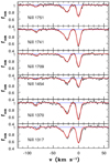 |
Fig. 3. Intervening Ni II absorption at zabs ≈ 2.40 in the HE 0027–1836 spectrum (black curves) and simultaneous fit to the main six transitions (red curves), using our f-values. At vhelio = 0 km s−1, the redshift is z = 2.40185. |
This system is the only one for which the weaker Ni IIλ1393 transition is detected. The latter displays a (nearly) unblended line profile appearing on the blue end of the strong Si IVλ1393 absorption from the same system. In Fig. 4, we show the fit (χ2 = 1.26) obtained for this Ni II transition (using the N and b parameters for the four velocity components corresponding to the results presented in Fig. 3) together with a fit of the very extended Si IV absorption. The latter extends over 300 km s−1; we do not show the profile at v > 130 km s−1, where Si IVλ1393 is heavily blended with Fe IIλ2344 multiple absorption at zabs = 1.023.
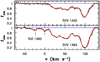 |
Fig. 4. Two Ni IIλ1393 absorption lines towards HE 0027–1836 at zabs = 2.40156 and 2.40185, occurring on the blue end of the extended Si IVλ1393 absorption (lower panel) together with the corresponding Si IVλ1402 profile (upper panel). The fit (red curve) obtained with our Ni IIλ1393 f-value is superimposed onto the observed spectrum (black line). At vhelio = 0 km s−1, the redshift is z = 2.40185. |
The fits for the three weak Ni II transitions at 1703, 1773, and 1804 Å (using N and b parameters derived from the six transitions shown in Fig. 3) are also presented in Fig. 5.
4.1.2. FBQS J0812+3208: the Ni II system at zabs=2.0668
For the strong transitions in this system, line fitting is required given the narrow profiles observed. Two Gaussian velocity components are sufficient to reproduce them, as illustrated in Fig. 6 where the simultaneous fit to the six strongest transitions obtained with our estimated f-values is shown, superimposed onto the observed profiles. As can be seen, the fit is quite satisfactory (χ2 = 1.29).
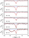 |
Fig. 6. Intervening Ni II absorption at z ≈ 2.06 towards the quasar FBQS J0812+3208 spectrum (black curves) and simultaneous fit to the main six transitions (red curves), using our f-values. Blueward of Ni IIλ1317, there is a Lyα absorption at z = 2.32260. At vhelio = 0 km s−1, the redshift is z = 2.06683. |
The well-detected weak transitions at 1467.2, 1467.7, and 1502 Å are used to derive our f-value estimates through equivalent width measurements. Adopting the N and b parameters inferred from the previous fit, the observed profiles can be adequately reproduced (χ2 = 1.08), as shown in Fig. 7, where we also display the fit to the λ1703 profile (the f-value of which has been derived from other systems).
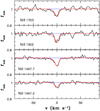 |
Fig. 7. Weak intervening Ni II absorption at z ≈ 2.06 in the FBQS J0812+3208 spectrum (black line) using the N and b parameters obtained from fitting of the four 1370, 1709, 141, and 1751 Å transitions shown in Fig. 6 (red curve). At vhelio = 0 km s−1, the redshift is z = 2.06683. |
4.1.3. FBQS J0812+3208: the Ni II system at zabs=2.6263
This system is used to constrain the f(1751)/f(1741) ratio (with the AOD method), and thus to determine f(1741) and f(1751). It also provides the most reliable estimate for the λ1317, λ1370, and λ1454 transitions. The simultaneous fit to these five strong transitions is good (χ2 = 0.95), as can be seen in Fig. 8 (eight velocity components are required to reproduce the relatively broad profiles). This system also allows us to constrain the λ1703 f-value and provides a test for the λ1502 and λ1370 results inferred from the low redshift system.
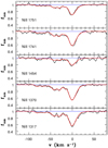 |
Fig. 8. Intervening Ni II absorption at z ≈ 2.62 towards the quasar FBQS J0812+3208 spectrum (black curves) and simultaneous fit to the main five transitions (red curves), using our f-values. At vhelio = 0 km s−1, the redshift is z = 2.62631. |
4.1.4. TXS 1331+170: the Ni II system at zabs=1.7764
Although the peak opacity in this system is less than in the four others (see Fig. 1), the excellent quality of the spectrum together with the absence of narrow velocity components in the observed profiles allow us to get valuable constraints on the f(1709)/f(1741) and f(1751)/f(1741) ratios. This system also provides a good test for the f(1317) and f(1370) values. The simultaneous fit to these transitions presented in Fig. 9 involves five velocity components: a good match to the data is obtained (χ2 = 1.29) using the f-values listed in Table 4.
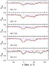 |
Fig. 9. Intervening Ni II absorption at zabs ≈ 1.77 in the TXS 1331+170 spectrum (black curve) and simultaneous fit to the four 1370, 1709, 1741, and 1751 Å transitions (red curve), using our estimated f-values. This fit is overlaid on the Ni IIλ1317 absorption profile, which is affected by weak Lyα absorptions blueward and redward of the main component. At vhelio = 0 km s−1, the redshift is z = 1.77638 |
4.1.5. LBQS 2206–1958: the Ni II system at zabs=1.9200
As illustrated by Fig. 2, the AOD method provides reliable f-value ratios over most of the absorption profile (v > 20 km s−1) for the 1317, 1370, 1703, 1709, 1741, and 1751 Å transitions, while the unresolved component at v = 0 km s−1 requires line fitting (or W measurements for optically thin lines). The simultaneous fit to the five strongest transitions (all the above except λ1703) shown in Fig. 10 is satisfactory (χ2 = 1.38); nine velocity components are needed to synthesise the whole profile. The match is also good for the 1703 Å transition, which f-value is derived from both this system and that in FBQS J0812+3208 at zabs = 2.6263.
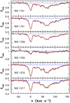 |
Fig. 10. Intervening Ni II absorption at zabs ≈ 1.92 in the LBQS 2206-1958 spectrum (black) and simultaneous fit to the main five strongest transitions (red curves), using our f-values. This fit is overlaid on the weaker Ni IIλ1703 transition. At vhelio = 0 km s−1, the redshift is z = 1.9200. |
Equivalent width measurements of the narrow component for the 1773 and 1804 Å absorption lines provide the adopted f-value for these two transitions. The corresponding fits are shown in Fig. 11 (χ2 = 1.53). To conclude this section, we note that the f-values listed in Table 4 are consistent with all constraints provided by the five systems considered in our study.
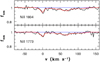 |
Fig. 11. Same as in Fig. 10 but for the two weak 1773 and 1804 Å transitions. The N and b parameters adopted are those derived from fitting of the 1317, 1370, 1709, 1741, and 1751 Å profiles shown in Fig. 10. |
4.2. Comparison with previously determined values
As noted earlier, our results for the three primary transitions at 1709, 1741, and 1751 Å are well consistent with those of Fedchak et al. (2000) and the largest relative difference is of +1.9% for the transition at 1709 Å; in this section, the relative differences considered are (f′−f)/f, where f′ is the already published value and f that obtained from this work. Since both sets of values are based on the absolute measurements of Fedchak & Lawler (1999) this means that the constraints obtained on relative values from our analysis of quasar systems are in good agreement with those drawn from laboratory work by Fedchak et al. (2000). The match is less good for the four additional transitions (at 1454, 1467.2, 1467.7, and 1703 Å) considered by Fedchak et al. (2000); the relative differences are +47%, +57%, +48%, and +11% respectively. Nevertheless, the two sets of results are mutually compatible given the relatively large uncertainties involved.
Zsargó & Federman (1998) studied the relative f-values of 12 Ni II transitions, of which six are within our list. As noted earlier, these values are to be rescaled according to the laboratory measurements of Fedchak & Lawler (1999). Thus, we compare our results to values from Zsargó & Federman (1998) multiplied by 0.534. The largest relative difference amounts to +50% for the 1467.2 Å transition, while most values are of about 10–20%. Since Zsargó & Federman (1998) do not quote uncertainties, a more detailed comparison is not possible.
Jenkins & Tripp (2006) investigated the three UV transitions at 1317, 1370, and 1454 Å and determined f-values with an accuracy of about 10%. Our results are in good agreement given the errors (relative differences are −4%, −5%, and +18%, respectively).
For species displaying a complex level structure such as Ni II, theoretical calculations are not expected to provide accurate f-values. Indeed, considering the most recent work of Cassidy et al. (2016; their calculation B results using the length gauge), we find that f-values are systematically overestimated, sometimes by as much as 100%: the median value of f′/f computed over the 13 transitions is 1.32 and the whole range covered by f′/f is 1.130–2.31. Considering the earlier values listed by Morton (1991) who refers to calculations performed by R. L. Kurucz, we note that the discrepancy was even more pronounced with a median value of f′/f reaching 2.26 (whole range : 1.48–3.39). Nevertheless, we stress that these theoretical values play an essential role in that they allow us to pinpoint the few transitions that may be detectable in astrophysical spectra. In particular, the three weak transitions at 1502, 1773, and 1804 Å investigated in this work have been identified in our spectra on the basis of the results published by Morton (1991) and Cassidy et al. (2016). We conclude this section by noting that our set of Ni IIf-values is consistent with all previous measurements and represents a significant improvement in accuracy.
5. Discussion and conclusions
5.1. Using QSO spectra to constrain f-values
Our work illustrates well the potential and the difficulties of using QSO spectra to derive relative f-values from astronomical data. As compared to hot stars, distant quasars with their high redshift absorption systems, offer the great advantage of providing opacity measurements for UV transitions using ground-based 8–10 m class telescopes. Another advantage of quasar absorption systems over interstellar lines is that the absorption profile induced by ions associated with DLAs often extends over an interval of 100 km s−1 or more (three of the five systems in our study are of this type), leading to a direct, unbiased estimate of the opacity. However, for such broad features, difficulties might be encountered because of the complex shape of quasar continua, resulting in significant uncertainties when normalising the spectrum in regions where emission features are present. In fact, for the systems considered in this study, this turned out not to be a real problem, except when dealing with weak features, such as those at 1773 and 1804 Å in LBQS 2206–1958. For such lines, uncertainties in the placement of the continuum become dominant and furthermore they are difficult to quantify.
When using quasar absorption lines to derive relative f-values, we can wonder which systems are best suited to provide the highest accuracy. Regarding resolved profiles, the reasoning presented in Boissé et al. (2015) applies (see their relation 6), and we can easily show that the largest response to a small difference in f (i.e. the optimal sensitivity expressed in terms of δIn/(δf/f), where In is the normalised intensity) is obtained for τ = 1 (or In = 0.37) and remains good in a relatively broad opacity interval τ ≈ 0.6 − 1.5 (corresponding to In ≈ 0.2 − 0.5). The absorption lines considered in this work fall on the low end of this opacity interval, even for the strongest transitions; this is especially true for the system in TXS 1331+170, which could provide information only on the strongest Ni II transitions. Concerning narrow unresolved lines, the optically thin ones – such as those associated with the 1502, 1773, and 1804 Å transitions considered above – are also well suited in that they too provide constraints that are free of any assumption on the velocity distribution. In this case, the best lines are those with the smallest relative uncertainty on the equivalent width, δW/W, since δf/f = δW/W.
5.2. Completeness of our study of Ni II transitions
In the list published by Morton (1991) and Cassidy et al. (2016), a few transitions have an f-value comparable to those of the weakest ones detected in our five absorption systems. This is true in particular for the two transitions at 1345.88 and 1412.86 Å. After careful examination of the spectra, we conclude that neither of these transitions is present in the systems where they could have been seen. For the 1345.88 Å transition, the best system is that at zabs = 2.6263 in FBQS J0812+3208 while the situation is the most favourable for the 1412.86 Å transition at zabs = 2.4018 in HE 0027–1836; for other systems, the expected line lies in a gap or in the Lyα forest or is blended with another feature. These two transitions fall near the low end of the rest wavelength range considered, corresponding to observed wavelengths in the bluest part of the spectra where the S/N ratio is generally lower. It is thus not surprising that these transitions remain undetected although their f-value is apparently similar to those of the 1773 and 1804 Å transitions. Thus, insofar as we have not missed transitions for which the theoretical f-value would have been grossly underestimated, we can consider that our survey of Ni II lines in the data considered in this work is complete.
5.3. Prospects for other species
For many other species of astrophysical interest in the context of interstellar or DLA studies, the accuracy of f-values is still limited. An overview of the present situation can be found in the recent compilation provided by Cashman et al. (2017) who have given an “accuracy grade” for f-values of many ions. As the S/N ratio characterising distant quasar spectra increases, more accurate measurements of absorption profiles can be made, leading to improved relative f-values. Further, weaker lines will become detectable resulting in new f-values for the corresponding transitions, which can then be used to get more reliable column density estimates. Finally, some additional elements (such as cobalt for which Co II displays ten transitions in the 1424–2059 Å interval: see e.g. Ellison et al. 2001b; Noterdaeme et al. 2015 for marginal detections) can become accessible, allowing us to extend the set of metals for which the relative abundance can be measured. If the f-value of their transitions is not well established, an approach like that presented in this paper can be developed.
Increasing the spectral resolution is also essential. Indeed, high redshift quasars generally display several absorption systems and blends of lines formed at distinct redshifts are frequent, as illustrated in this work. Moreover, a higher spectral resolution increases the fraction of absorption profiles for which the opacity can be measured directly. For instance, the new ESPRESSO spectrograph mounted on the ESO/VLT (Pepe et al. 2013), is expected to provide spectra of bright quasars with a resolution improved by a factor of at least two as compared to that provided by UVES or HIRES. In any case, it is important to keep in mind that we necessarily need to rely on good theoretical estimates of f-values to guide work at the laboratory or on astronomical spectra and laboratory determinations of the f-value for at least a few transitions to establish an absolute scale, to be used once relative f-values have been determined.
5.4. Conclusions
In this paper, we investigate absorption lines associated with UV Ni II transitions in five high redshift systems to derive their relative f-value. We adopt two methods which are free of any assumption on the gas velocity distribution: first a direct estimate of the opacity applied to fully resolved and unblended portions of the absorption profiles (AOD method), and second equivalent width measurements of optically thin lines. Absolute f-values are then obtained by combining our results to the absolute laboratory measurements performed by Fedchak & Lawler (1999). Line fitting has also been used to verify that the set of f-values thus obtained is consistent with all observed absorption profiles, including blended or unresolved ones. In this way, we could significantly improve the accuracy of the f-value for ten transitions that have already been investigated (the median relative accuracy is now 6.5%) and measure for the first time, the strength of three weak transitions that have not been detected earlier in astronomical spectra. These results provide a solid basis for accurate determinations of N(Ni II) in the interstellar medium or in quasar DLA systems to be used in particular for nucleosynthesis or dust depletion studies.
Acknowledgments
We are grateful to Pasquier Noterdaeme for pointing out the value of quasar absorption systems to improve the accuracy of Ni IIf-values and to Hadi Rahmani for providing the excellent spectrum of HE 0027–1836. Discussions with Ben Wandelt about the appropriate way to use constraints on f-value ratios have been very helpful. We also thank Steve Federman and Jim Lawler for several fruitful discussions about some aspects of f-values measurements. Finally, we are grateful to the anonymous referee, whose thorough comments helped us to improve the clarity of this paper.
References
- Balashev, S. A., Noterdaeme, P., Klimenko, V. V., et al. 2015, A&A, 575, L8 [Google Scholar]
- Balashev, S. A., Noterdaeme, P., Rahmani, H., et al. 2017, MNRAS, 470, 2890 [NASA ADS] [CrossRef] [Google Scholar]
- Bergeron, J., & Boissé, P. 2017, A&A, 604, A37 [NASA ADS] [CrossRef] [EDP Sciences] [Google Scholar]
- Bergeron, J., & Petitjean, P. 1991, A&A, 241, 365 [NASA ADS] [Google Scholar]
- Bergeron, J., Petitjean, P., Aracil, B., et al. 2004, The Messenger, 118, 40 [NASA ADS] [Google Scholar]
- Boissé, P., Bergeron, J., Prochaska, J. X., Péroux, C., & York, D. G. 2015, A&A, 581, A109 [NASA ADS] [CrossRef] [EDP Sciences] [Google Scholar]
- Carswell, R. F., Jorgenson, R. A., Wolfe, A., & Murphy, M. T. 2011, MNRAS, 411, 2319 [NASA ADS] [CrossRef] [Google Scholar]
- Cashman, F. H., Kulkarni, V. P., Kisielius, R., Ferland, G. J., & Bogdanovich, P. 2017, ApJS, 230, 8 [NASA ADS] [CrossRef] [Google Scholar]
- Cassidy, C. M., Hibbert, A., & Ramsbottom, C. A. 2016, A&A, 587, A107 [NASA ADS] [CrossRef] [EDP Sciences] [Google Scholar]
- Dessauges-Zavadsky, M., Prochaska, J. X., D’Odorico, S., Calura, F., & Matteucci, F. 2006, A&A, 445, 93 [NASA ADS] [CrossRef] [EDP Sciences] [Google Scholar]
- Ellison, S. L., Pettini, M., Steidel, C. C., & Shapley, A. E. 2001a, ApJ, 549, 770 [NASA ADS] [CrossRef] [Google Scholar]
- Ellison, S. L., Ryan, S. G., & Prochaska, J. X. 2001b, MNRAS, 326, 628 [NASA ADS] [CrossRef] [Google Scholar]
- Fedchak, J. A., & Lawler, J. E. 1999, ApJ, 523, 734 [NASA ADS] [CrossRef] [Google Scholar]
- Fedchak, J. A., Wiese, L. M., & Lawler, J. E. 2000, ApJ, 538, 773 [NASA ADS] [CrossRef] [Google Scholar]
- Federman, S. R., & Zsargó, J. 2001, ApJ, 555, 1020 [NASA ADS] [CrossRef] [Google Scholar]
- Jenkins, E. B., & Tripp, T. M. 2006, ApJ, 637, 552 [NASA ADS] [CrossRef] [Google Scholar]
- Jorgenson, R. A., Wolfe, A. M., Prochaska, J. X., & Carswell, R. F. 2009, ApJ, 704, 247 [NASA ADS] [CrossRef] [Google Scholar]
- Jorgenson, R. A., Wolfe, A. M., & Prochaska, J. X. 2010, ApJ, 722, 460 [NASA ADS] [CrossRef] [Google Scholar]
- Molaro, P., Centurión, M., Whitmore, J. B., et al. 2013, A&A, 555, A68 [NASA ADS] [CrossRef] [EDP Sciences] [Google Scholar]
- Morton, D. C. 1991, ApJS, 77, 119 [NASA ADS] [CrossRef] [Google Scholar]
- Morton, D. C. 2003, ApJS, 149, 205 [NASA ADS] [CrossRef] [MathSciNet] [Google Scholar]
- Noterdaeme, P., Ledoux, C., Petitjean, P., et al. 2007, A&A, 474, 393 [Google Scholar]
- Noterdaeme, P., Srianand, R., Rahmani, H., et al. 2015, A&A, 577, A24 [NASA ADS] [CrossRef] [EDP Sciences] [Google Scholar]
- O’Meara, J. M., Lehner, N., Howk, J. C., et al. 2015, AJ, 150, 111 [NASA ADS] [CrossRef] [Google Scholar]
- Pepe, F., Cristiani, S., Rebolo, R., et al. 2013, The Messenger, 153, 6 [NASA ADS] [Google Scholar]
- Pettini, M., Hunstead, R. W., & Smith, 1990, MNRAS, 246, 545 [NASA ADS] [Google Scholar]
- Pettini, M., Smith, L. J., Hunstead, R. W., & King, D. L. 1994, ApJ, 426, 79 [NASA ADS] [CrossRef] [Google Scholar]
- Prochaska, J. X., Howk, J. C., & Wolfe, A. 2003, Nature, 423, 57 [NASA ADS] [CrossRef] [PubMed] [Google Scholar]
- Prochaska, J. X., & Wolfe, A. M. 1997, ApJ, 474, 140 [NASA ADS] [CrossRef] [Google Scholar]
- Prochaska, J. X., Wolfe, A. M., Howk, J. C., et al. 2007, ApJS, 171, 29 [NASA ADS] [CrossRef] [Google Scholar]
- Rahmani, H., Wendt, M., Srianand, R., et al. 2013, MNRAS, 435, 861 [NASA ADS] [CrossRef] [Google Scholar]
- Rauch, M., Carswell, R. F., Webb, J. K., & Weymann, R. J. 1993, MNRAS, 260, 589 [NASA ADS] [CrossRef] [Google Scholar]
- Savage, B. D., & Sembach, K. R. 1991, ApJ, 379, 245 [NASA ADS] [CrossRef] [Google Scholar]
- Wolfe, A. M., Gawiser, E., & Prochaska, J. X. 2005, ARA&A, 43, 861 [NASA ADS] [CrossRef] [MathSciNet] [Google Scholar]
- Zsargó, J., & Federman, S. R. 1998, ApJ, 498, 256 [NASA ADS] [CrossRef] [Google Scholar]
All Tables
All Figures
|
Fig. 1. Ni IIλ1741 absorption profile for the five systems considered in this study. The redshift of the strongest narrow absorption feature is indicated at the lower left corner of each panel and corresponds to vhelio = 0 km s−1. All features appearing in these profiles are from the Ni IIλ1741 transition except that shaded in the middle panel. |
| In the text | |
|
Fig. 2. Intervening Ni II absorption towards the quasar LBQS 2206–1958 at za ≈ 1.92. The opacity profiles for the 1317 (thin black line), 1370 (red), 1703 (green), 1709 (blue), 1741 (thick black), and 1751 Å (cyan) transitions are shown in the upper panel. The ratio of any given profile to the 1741 Å profile is shown in the lower panel. The ratios are better defined at velocities for which the opacity is large; they range from 0.125 (for 1703 Å) up to 1.43 (1370 Å), thus covering a dynamical range of 11.4. At vhelio = 0 km s−1, the redshift is za = 1.9200. |
| In the text | |
|
Fig. 3. Intervening Ni II absorption at zabs ≈ 2.40 in the HE 0027–1836 spectrum (black curves) and simultaneous fit to the main six transitions (red curves), using our f-values. At vhelio = 0 km s−1, the redshift is z = 2.40185. |
| In the text | |
|
Fig. 4. Two Ni IIλ1393 absorption lines towards HE 0027–1836 at zabs = 2.40156 and 2.40185, occurring on the blue end of the extended Si IVλ1393 absorption (lower panel) together with the corresponding Si IVλ1402 profile (upper panel). The fit (red curve) obtained with our Ni IIλ1393 f-value is superimposed onto the observed spectrum (black line). At vhelio = 0 km s−1, the redshift is z = 2.40185. |
| In the text | |
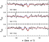 |
Fig. 5. Same as in Fig. 3 for HE 0027–1836 but for the three 1703, 1773, and 1804 Å transitions. |
| In the text | |
|
Fig. 6. Intervening Ni II absorption at z ≈ 2.06 towards the quasar FBQS J0812+3208 spectrum (black curves) and simultaneous fit to the main six transitions (red curves), using our f-values. Blueward of Ni IIλ1317, there is a Lyα absorption at z = 2.32260. At vhelio = 0 km s−1, the redshift is z = 2.06683. |
| In the text | |
|
Fig. 7. Weak intervening Ni II absorption at z ≈ 2.06 in the FBQS J0812+3208 spectrum (black line) using the N and b parameters obtained from fitting of the four 1370, 1709, 141, and 1751 Å transitions shown in Fig. 6 (red curve). At vhelio = 0 km s−1, the redshift is z = 2.06683. |
| In the text | |
|
Fig. 8. Intervening Ni II absorption at z ≈ 2.62 towards the quasar FBQS J0812+3208 spectrum (black curves) and simultaneous fit to the main five transitions (red curves), using our f-values. At vhelio = 0 km s−1, the redshift is z = 2.62631. |
| In the text | |
|
Fig. 9. Intervening Ni II absorption at zabs ≈ 1.77 in the TXS 1331+170 spectrum (black curve) and simultaneous fit to the four 1370, 1709, 1741, and 1751 Å transitions (red curve), using our estimated f-values. This fit is overlaid on the Ni IIλ1317 absorption profile, which is affected by weak Lyα absorptions blueward and redward of the main component. At vhelio = 0 km s−1, the redshift is z = 1.77638 |
| In the text | |
|
Fig. 10. Intervening Ni II absorption at zabs ≈ 1.92 in the LBQS 2206-1958 spectrum (black) and simultaneous fit to the main five strongest transitions (red curves), using our f-values. This fit is overlaid on the weaker Ni IIλ1703 transition. At vhelio = 0 km s−1, the redshift is z = 1.9200. |
| In the text | |
|
Fig. 11. Same as in Fig. 10 but for the two weak 1773 and 1804 Å transitions. The N and b parameters adopted are those derived from fitting of the 1317, 1370, 1709, 1741, and 1751 Å profiles shown in Fig. 10. |
| In the text | |
Current usage metrics show cumulative count of Article Views (full-text article views including HTML views, PDF and ePub downloads, according to the available data) and Abstracts Views on Vision4Press platform.
Data correspond to usage on the plateform after 2015. The current usage metrics is available 48-96 hours after online publication and is updated daily on week days.
Initial download of the metrics may take a while.