| Issue |
A&A
Volume 622, February 2019
|
|
|---|---|---|
| Article Number | A65 | |
| Number of page(s) | 14 | |
| Section | Galactic structure, stellar clusters and populations | |
| DOI | https://doi.org/10.1051/0004-6361/201834103 | |
| Published online | 29 January 2019 | |
On collision course: The nature of the binary star cluster NGC2006/SL 538
Institute of Astrophysics, Pontificia Universidad Católica de Chile, Av. Vicuña Mackenna 4860, 7820436 Macul, Santiago, Chile
e-mail: This email address is being protected from spambots. You need JavaScript enabled to view it.
Received:
17
August
2018
Accepted:
15
November
2018
Abstract
Context. The Large Magellanic Cloud (LMC) is known to be the host of a rich variety of star clusters of all ages. A large number of them is seen in close projected proximity. Ages have been derived for few of them showing differences up to few million years, hinting at being binary star clusters. However, final confirmation through spectroscopy measurements and dynamical analysis is needed.
Aims. In the present work we focus on one of these LMC cluster pairs (NGC 2006–SL 538) and aim to determine whether the star cluster pair is a bound entity and, therefore, a binary star cluster or a chance alignment.
Methods. We used the Magellan Inamori Kyocera Echelle (MIKE) high-resolution spectrograph on the 6.5 m Magellan-II Clay telescope at Las Campanas Observatory to acquire integrated-light spectra of the two clusters, measuring their radial velocities with individual absorption features and cross-correlation of each spectrum with a stellar spectral library.
Results. We measured radial velocities by two methods: first by direct line-profile measurement yields νr = 300.3 ± 5 ± 6 km s−1 for NGC 2006 and νr = 310.2 ± 4 ± 6 km s−1 for SL 538. The second one is derived by comparing observed spectra with synthetic bootstrapped spectra yielding νr = 311.0 ± 0.6 km s−1 for NGC 2006 and νr = 309.4 ± 0.5 km s−1 for SL 538. Finally when spectra are directly compared, we find a Δν = 1.08 ± 0.47 km s−1. Full-spectrum spectral energy distribution fits reveal that the stellar population ages of both clusters lie in the range 13–21 Myr with a metallicity of Z = 0.008. We find indications for differences in the chemical abundance patterns as revealed by the helium absorption lines between the two clusters. The dynamical analysis of the system shows that the two clusters are likely to merge within the next ∼150 Myr to form a star cluster with a stellar mass of ∼104 M⊙.
Conclusions. The NGC 2006–SL 538 cluster pair shows radial velocities, stellar population and dynamical parameters consistent with a gravitational bound entity and, considering that the velocity dispersion of the stars in LMC is ≲20 km s−1, we reject them as a chance alignment. We conclude that this is a genuine binary cluster pair, and we propose that their differences in ages and stellar population chemistry is most likely due to variances in their chemical enrichment history within their environment. We suggest that they may have formed in a loosely bound star-formation complex which saw initial fragmentation but then had its clusters become a gravitationally bound pair by tidal capture.
Key words: galaxies: individual: LMC / galaxies: star clusters: individual: NGC 2006 / galaxies: star clusters: individual: SL 538
© ESO 2019
1. Introduction
In the context of star cluster formation, it is known that star clusters form in large fractal entities where interactions between subclusters of various masses are likely. These interactions are short and violent processes that happen at the youngest stages of star cluster evolution and last for a few to a few tens of millions of years (Sugimoto & Makino 1989; Yu et al. 2017). Such processes may lead to star cluster disruption or star cluster merging (e.g., Kroupa 1998; Fellhauer & Kroupa 2005). A snapshot of this short-living stage may be observed as two star clusters in close projected proximity to each other on the sky (i.e.,star cluster pairs). Such pairs may then be considered binary star clusters if their relative velocities are consistent with being gravitationally bound systems.
The origin of binary clusters, as proposed by (Fujimoto & Kumai 1997), is a parent gas cloud that fragments in at least two separate subclumps, yielding two or more bound star clusters of virtually identical ages and abundances. However, it is also possible that binary star clusters form by tidal capture (Leon et al. 1999), where clusters born in different clouds (thus likely having different ages and abundances) later become a bound system due to a close encounter and subsequent loss of angular momentum. If these subclusters are gravitationally bound, they will eventually merge and form a more massive star cluster, mixing the constituent stellar populations of the subclusters. Such processes are a possible scenario leading to globular clusters with multiple stellar populations (Gratton et al. 2012), which is likely to happen in dwarf galaxies where the stellar velocity dispersion within the galaxy is comparable to that within the globular clusters, for example, Sagittarius dwarf (Bellazzini et al. 2008), and the Magellanic clouds (e.g., Bhatia & Hatzidimitriou 1988).
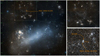 |
Fig. 1. Overview of the Large Magellanic Cloud (LMC) and the location, environment and morphology of the NGC 2006 (SL 539) and SL 538 star cluster pair. The figures are based on DSS colored images. Left panel: an overview of the LMC with the location of NGC 2006/SL 539 indicated by the arrow. The dashed square shows the outline of the zoom-in image in the top right panel, which illustrates the environment of the double star cluster. Bottom right panel: star cluster pair, separated by ∼13pc, within the stellar field of the immediate environment. |
The Magellanic clouds host several star-cluster pairs whose stellar populations have been analyzed photometrically by means of color-magnitude diagrams (e.g., Bhatia & Hatzidimitriou 1988; Hatzidimitriou & Bhatia 1990; Bhatia et al. 1991; Pietrzynski & Udalski 1999). For example, Dieball & Grebel (2000) concluded that the pair NGC 1971 & NGC 1972 have similar ages (40–70 Myr) indicating that both clusters may have been formed in the same giant molecular cloud. However, they could not establish whether the clusters are physically interacting. They also found that NGC 1894 & SL 341 show similar ages (55 ± 5 Myr), concluding that the formation of both clusters from the same giant molecular cloud is likely. Using Strömgren CCD photometry Hilker et al. (1995) found that NGC 2136 & NGC 2137 have common metallicities (−0.55 dex), also their color magnitude diagrams lie along the same isochrone and, therefore, the ages of the two star clusters cannot be distinguished, concluding that the simultaneous formation is likely. Later Dirsch et al. (2000) derived an age of 100 ± 25 Myr for this star cluster pair. Dieball & Grebel (2000) combined stellar photometry of SL 353 and SL 349 with spectroscopic measurements for 22 stars on both clusters and found an age of 500 ± 100 Myr for both clusters and radial velocities of ν = 274 ± 4 and ν = 279 ± 19 km s−1 for SL 353 and SL 349, respectively. They argue that the small velocity difference and similar ages are consistent with a gravitationally bound star cluster pair. Recently, (Mucciarelli et al. 2012) have found radial velocities ν = 271.5±0.4 and 270.6±0.5 km s−1 for NGC2136 and NGC 2137, and indistinguishable abundance patterns [Fe/H] = -0.40 ± 0.01 and -0.39 ± 0.01 dex, respectively. Based on the numerical simulations of this system performed by Portegies Zwart & Rusli (2007), the orbital parameters indicate that a merger is expected on a timescale comparable to the orbital period of these clusters.
The star cluster pair NGC 2006 (SL 539)/SL 538 (see Fig. 1) is located in the outskirts of the Large Magellanic Cloud (LMC) and is one of the many such pairs detected in the LMC (Dieball et al. 2002). Both clusters are seen at a projected distance of 13.3 pc (Dieball & Grebel 1998), and are located in the supergiant shell LMC4, at the northwestern part of the OB association LH77. Several authors have measured ages of 22.5 ± 2.5 Myr (Dieball & Grebel 1998) and 25 ± 3 Myr (Kumar et al. 2008) for NGC 2006, while SL 538 was found to have ages of 18±2 Myr (Dieball & Grebel 1998) and 20±2 Myr (Kumar et al. 2008). Both clusters were reported as binary clusters by Kontizas et al. (1993) through the analysis of the cores of the clusters using low-resolution prism spectra and integrated IUE spectra. The LMC is not the only galaxy hosting confirmed and likely binary clusters. For example, (De Silva et al. 2015) reported the open cluster pair NGC 5617/Trumpet 22 as primordial binary cluster pair in the Milky Way, while likely binary clusters have also been found in NGC5128 (Minniti et al. 2004). Therefore, binary star clusters are being detected in more galaxies with recent or ongoing star-formation activity. Whether they are a common entity or not needs to be investigated in greater detail.
For a cluster pair to be considered a binary star cluster, it must fulfill the following conditions: Both clusters must be seen as a star cluster pair (i.e.,in close projected proximity). Clusters may share similar (or different) ages and abundances (under the assumption of a common (or different) original cloud), and a difference in radial velocity of few km s−1. Under these criteria, if a star cluster pair such as NGC2006 (SL 539)/SL 538 in the LMC is bound (assuming masses of the order 104 M⊙) the expected orbital velocity correspond indeed to a few km s−1, which in low-resolution spectra will be seen as identical velocities (e.g., Kontizas et al. 1993). For younger stellar populations, and by inference for younger star clusters, the velocity dispersion is lower at about σ ≈ 20 km s−1 (e.g., van der Marel et al. 2002). On the other hand, if the star cluster pair is a chance alignment the radial velocity difference is expected to be consistent with the stellar field velocity dispersion of the younger stellar population in the LMC (i.e., likely smaller than 20 km s−1; see van der Marel et al. 2002). Thus, in order to move one step toward the confirmation of binarity (or its rejection) high-resolution spectroscopy is required to accurately measure radial velocities with km s−1 accuracy and distinguish between these two scenarios. This is done by Mucciarelli et al. (2012) in the case of the star cluster pair NGC2136/2137 which led to the confirmation of its binary status. In this work we present the kinematic analysis of the cluster pair NGC2006 (SL 539)/SL 538 using high-resolution spectra with the aim of constraining whether this pair is a bound system. Our paper is structured as follows: in Sect. 2 we describe the observations, while in Sect. 3 we describe the data reduction. Section 4 describes our analysis and finally in Sect. 5 we discuss the results and present our conclusions.
 |
Fig. 2. Example of an arc frame from the MIKE spectrograph. We note that individual orders are heavily curved, as is typical for echelle spectra, in addition to a substantial tilt of the emission lines within each order that changes as a function of wavelength. |
2. Observations
Spectra were acquired during the night of December 10th, 2013 with the Magellan Inamori Kyocera Echelle (MIKE) spectrograph mounted on the Magellan-II Clay telescope, located at Las Campanas Observatory in Chile. The instrument setup was using the 0.7″×5.0″ slit and the CCD readout was binned in 2×2 pixels, which yields a spectral resolution of ∼30 000 in the blue part of the spectrum. The wavelength coverage spans 3600–9000 Å. The night was photometric with a seeing of ∼0.6″. For each cluster we pointed toward the central part and applied a random jitter inside the central cluster area without closing the shutter with the aim of obtaining a representative sample of the stellar population of each cluster. Three exposures of 900 s were taken for each cluster and one exposure of 900 s in a nearby empty field with the aim of deriving and subtracting the average integrated-light spectrum of the sky and background.
3. Data reduction
High-resolution echelle spectra require careful data reduction in order to obtain the best radial velocity results of the star cluster pair. One of the critical issues regarding echelle data reduction is the correction of the individual orders which are typically heavily curved. In the case of our MIKE spectrograph, the instrument optics introduces an additional tilt of the wavelength solution within one order, as can be seen in an arc frame shown in Fig. 2. Our integrated-light spectra require the use of the entire (fully illuminated) slit and not only the trace of a point source, as is traditionally done in spectroscopic observations. Accurate correction of the differential wavelength calibration of every pixel in Fig. 2 is necessary before collapsing the order into a 1D spectrum. Without such a correction absorption and emission features would be washed out and spectral resolution would be lost, and in the most extreme cases, the features might appear to be double-peaked. In the following we describe a custom recipe that we developed to apply a pixel-by-pixel wavelength calibration to the individual echelle orders. We make this recipe publicly available1 and encourage comments and suggestions for improvement from the community.
The correction procedure assumes that the science frames are bias and flat-field corrected. We note that it is critical to acquire well-illuminated flat-field frames, even if it saturates some of the orders, however, not to the point of “bleeding”. Such flats are used to straighten out the individual orders. The idea is to use the order illumination patterns to map the optics curvature, which is then used to correct individual orders and transform them into rectified orders. Poorly illuminated orders can be successfully corrected after initially applying a smoothing function, which can enhance the order-edge detectability at the expense of cutting a fraction of the spatial extent of the sky. Before appliying our recipe, bias and flatfield corrected science frames were cosmic cleaned using the La-cosmic (van Dokkum 2001) routine.
3.1. Order edge detection and mapping
The first step uses the flat-field frames to identify and characterize the edges of the individual echelle orders. Poorly illuminated orders are smoothed along the x-axis (roughly corresponding to the dispersion axis) to obtain better defined edges. Once the order edges were sufficiently well defined, we applied a Sobel edge detection algorithm to the image along the y-axis using the ndimage.sobel SciPy task. This task creates a new image with highlighted order edges. This highlighted-edge image is then subtracted from the original flat-field frame creating a “pure-edge” image, which contains only information regarding the position of the edges. Finally, an (adjustable) minimum threshold of 500 “counts” is used to avoid inter-order features. The final product is a pure-edge image which corresponds to the science frame with zeros in the order and inter-order regions, except for the detected edges. Figure 3 illustrates a cut along the y-axis through the pure-edge image.
To map each order we used a simple Python script that extracts the order regions that lie in between the previously detected order edges and stores them in a look-up coordinate table. For each order the output is visually verified on the image to avoid spurious detections typically at the extreme ends along the dispersion direction in each order. This procedure works well for well illuminated orders, but it requires human interaction for order regions where the flat-field frame is poorly illuminated. Nevertheless, since the important information is stored in tables with the edge coordinates, if necessary it is still possible to cut, straighten, or extrapolate the orders manually.
3.2. Order rectification
The next step concerns the straightening of individual orders. For this purpose, we used the mapped edge coordinates of each order and use the IRAF task geomap to derive a transformation from the curved into the rectified frame. Since geomap requires the target coordinates to be specified, we adopt a uniform slit length of 26 pixels (5″ on the sky) in the target frame in order to preserve a uniform spatial scaling of the slit in each order. Since this is an interactive task, outliers can be easily corrected by deleting the corresponding points that are outside the regular shape of the curved order. We use a spline2 function with an order of three for the rectification. Finally, the Pyraf task gregister is used to execute the transformation with the option of flux conservation set to yes. An example of the final outcome from this process can be seen in the top panel of Fig. 4 where we show a straight order, however, still with a tilted wavelength solution.
3.3. Wavelength calibration and sky subtraction
Since the wavelength solution in the rectified frame is still tilted, meaning that the arc emission lines have not one of the same x-coordinates at any y-coordinate., a proper wavelength calibration of each pixel in the rectified order needs to be applied. This was done using the Pyraf task identify in a classical way, for each pixel row of each order. Typical root mean square (rms) values for the wavelength solutions were of the order of 0.4Å and the final dispersion correction was applied using the dispcor task. A rectified and wavelength calibrated frame is illustrated in the bottom panel of Fig. 4.
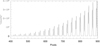 |
Fig. 3. Cut along the y-axis of the “pure-edge” image. Edge borders are indicated by positive count values and show a characteristic change in order width as a function of y-coordinate pixels, which corresponds to the spatial direction along the slit. |
3.4. Science spectra and sky subtraction
For each order, we summed all rows of the rectified and wavelength calibrated frames into a single object spectrum. In other words,we collapsed the 2D spectra into a combined 1D spectrum. Since three exposures were acquired for each cluster, the final step was the addition of these three collapsed spectra yielding the final science spectrum for each cluster.
Background subtraction was performed using the sky observations obtained with the corresponding science frames. For each order, we created an average combined master sky spectrum which was identically reduced as the science frames and accordingly scaled. These 1D sky spectra were then subtracted from the corresponding 1D science spectra.
4. Analysis
Prior to the kinematic analysis, we explore the individual orders and find that the most prominent spectral features are detected on the blue-side detector of MIKE, as it is expected for a young stellar population. Since we obtain a significantly higher signal-to-noise ratio (S/N) on the blue-side than on the red-side detector, we have focussed our subsequent analysis on the blue side of MIKE which samples the wavelength region of about 3600-5000 Å at a resolution of R ≈ 28 000 with a sampling of ∼0.04 Å pix−1.
The cluster spectra are consistent with a mixture of O–B type stars, in line with their approximate age of 20 Myr (Dieball & Grebel 1998; Kumar et al. 2008). We observe strong Balmer absorption and He i absorption features (see Fig. 5). Therefore, we used the aforementioned features to accurately measure the cluster radial velocities and to assess the validity of the bound binary cluster scenario. The selection of the weaker absorption features is somewhat arbitrary and is based on their position (i.e., at the central wavelength) within the corresponding echelle order. Since the transmission curves maximizes the S/N in approximately the center of each order along the dispersion axis (see Fig. 2), features near the borders of the individual orders are rejected from the following analysis due to their small S/N.
 |
Fig. 4. Example of the order rectification and wavelength calibration correction. Top panel: rectified order cutout of an arc frame, not wavelength calibrated. Bottom panel: wavelength calibrated arc frame. |
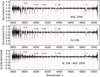 |
Fig. 5. Normalized integrated-light spectra for NGC 2006 ( top panel) and SL 538 ( middle panel). Bottom panel: difference spectrum (SL 538–NGC 2006). The vertical red lines in each panel mark the echelle order overlap regions. Some strong absorption features are labeled. |
4.1 Evaluation of the line profile shapes
In an attempt to select the best way of measuring the radial velocity from individual absorption features, we tested three different profiles: Gaussian, Moffat, and Voigt. A first estimate of the central wavelength position is measured using the IRAF task splot, which is then used as a starting point for the line profile fitting routine. The continuum near the absorption feature is mapped by a polynomial function of order nine, which is then subtracted from the spectra. Then the three profile types are fitted to the absorption features and the resulting fitting curve is subtracted from the data creating the residual spectra. This procedure is iterated until the solution converges (typically three times). Finally, we chose the best fitting profile by visual inspection of the residuals and conclude that the residuals from the Voigt profile are smaller than the residuals from the Moffat and Gaussian profiles. Therefore, we adopted the Voigt profile for deriving central wavelength positions for our absorption features.
Summary of the radial velocity measurements from individual absorption features in NGC 2006 and SL 538.
4.2 Radial velocity measurements
For the measured central wavelength positions (λm) of the studied absorption features we derive the corresponding radial velocity values (νr) and summarize the results in Table 1. The corresponding line fits for both clusters are shown in Fig. A.1. We observe a systematically larger radial velocity for SL 538 compared to NGC 2006 with an observed maximum λm difference for the Hδ line of 0.32 Å, corresponding to a radial velocity offset of Δνr ≃24 km s −1. We note that the largest offsets are measured for the lowest-S/N features with the largest uncertainties. Nevertheless, we observe that the large differences are consistent in the direction of the offset with the other features. At the bottom of Table 1, we show the final mean radial velocities for each cluster based on the individual Voigt profile fits.
In the following we have estimated the reliability of our measurements by bootstrapping the science spectra with their variance properties and repeating the measurements. To assess the external errors of our measurements, we varied each pixel value according to its random noise component. For each pixel we randomized its original value (N sci) by adding a random component, assuming 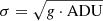 , where g = 0.47 is the MIKE blue arm gain in e−/ADU. Given the Poisson statistics and the original science spectrum a new artificial spectrum is generated, where for each pixel value we obtain
 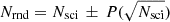 . Here
  is the Poisson distribution of each pixel value. We repeated this randomization and measurement procedure 10 000 times. Visual examples of the fittings are presented in Fig. A.1 and the measured radial velocity uncertainties are given in Table 1, where the first error corresponds to the measurement uncertainties taking into account the variations of each line due to profile fitting. The second error corresponds to the 95% minimum and maximum recovered values, taken from our bootstrapping experiments, assuming a Gaussian distribution. This external error represents the reliability of the individual profile fitting, which is finally estimated as the resulting value.
We find νr = 300.3 ±km s−1 with a bootstrap error of 4 km s−1 for NGC 2006 and νr = 310.2 ± 4 km s−1 and bootstrap error of 2 km s−1 for SL 538. The first errors correspond to the standard error of the mean for the statistical uncertainty, while the second bootstrap error is discussed above. Given our measurements we obtain a radial velocity difference estimate of Δνr = 10 ± 9 ±3 km s−1 (±stat±btstrp), which is larger much than zero radial velocity offset but still consistent with it within one-sigma uncertainties. We note that the radial velocities for both clusters are corrected for the heliocentric radial velocity at the time of the observations of Δνh = −1.6 km s−1. In general, SL 538 shows systematically smaller errors than NGC2006 and its measurements are more stable for features at redder wavelength, which is a consequence of the MIKE transmission curve.
4.3 Full spectrum cross correlation
An alternative to the measurement of the central wavelengths of individual absorption lines is the full-spectrum cross correlation with radial velocity template spectra. Before applying the cross-correlation technique to the NGC2006 and SL 538 spectra, we normalized each order and combine them into a master spectrum for each cluster showing the full wavelength coverage. Both spectra are shown in Fig. 5 together with their corresponding difference spectrum. It is obvious that the blue and red edges of these spectra are relatively noisy compared to the central portion around ∼3800–4900 Å which contain strong features that are well suited for cross-correlation. We have used these portions of the spectra as input for a relative velocity estimation with the TRAF task fxcorr, which is based on the cross-correlation algorithm of Tonry & Davis (1979). Direct cross-correlation of both spectra, meaning using one as input science and the other as template spectrum, yields a relative radial velocity of Δνr = 0.4 km s−1.
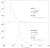 |
Fig. 6. Distribution of derived radial velocities from cross-correlation of the two target clusters and 1872 synthetic stellar template spectra from Coelho (2014). We note the differences in the asymmetric distributions of the resulting radial velocities, which indicates the degree of template mismatch for each cluster-template spectrum combination. |
Visual inspection of the normalized cluster spectra reveals some patterns that indicate that template mismatch might be a concern (see Fig. 5). We, therefore, choose a stellar spectrum library as reference in order to evaluate such systematics. For this, we are using 1872 high-resolution theoretical stellar spectra from the library of Coelho (2014) as radial-velocity templates for the fxcorr task. Figure 6 shows the histogram of the derived radial velocity distributions from the cross-correlation of the cluster spectra with the template library. The velocity distribution histograms for both clusters show similarly asymmetric, but not identical shapes, corroborating our suspicion that template mismatch is significant when auto-correlating the cluster spectra. We obtain for the two clusters an average radial velocity of 〈νr〉 = 311.51 ± 0.05km s−1 and 310.01 ± 0.02 km s−1 for NGC2006 and SL 538, respectively, with a dispersion of σ = 1.04 km s−1 for SL 538 and σ = 2.22 km s−1 for NGC2006, and corresponding median values of 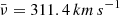 and
and  . Considering the derived values from the cross-correlation with the stellar template library we find a radial velocity difference between the two clusters of Δνr = 1.50 ± 0.07 km s−1.
However, the asymmetry of the distributions in Fig. 6 generated by the asymmetric absorption profile shapes of some features, in particular H-epsilon which blends with the Ca K+H lines. If template and object spectra show different relative feature strengths, asymmetric offsets in radial velocity will be produced. Moreover, this clearly shows that a proper selection of the standard star is critical, as a randomly chosen template may introduce velocity variations up to ∼3-4 km s−1. Histograms in Fig. 6 also show the preferred values at their peaks, that is, the most frequent velocity value, given the spectral types included in the stellar spectra library (Coelho 2014). However, since the library has different spectral types frequencies, the peaks could simply correspond to the most frequent ones, so we performed 10 000 random experiments where we randomly selected five templates for each stellar temperature and we look at the most common value, finding agreement between the peaks. The standard star types at or near the peaks of the histograms in Fig. 6 represent the best approximations to our cluster spectra.
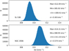 |
Fig. 7. Estimated radial velocity distributions for SL 538 ( top panel) and NGC2006 ( bottom panel) from cross-correlation of the bootstrapped cluster and the best-template stellar library spectra (see Sect. 4.3 for details). |
To assess the influence of the S/N of our cluster spectra independent of the template mismatch error, we have selected the best nine stellar library spectra, corresponding to stars of temperatures 5750–6000 K and consistent to be present in the peaks of our random experiments as well as in Fig. 6, as template radial velocity standards. Each template was transformed to the resolution of the observed spectra, and had proportional noise added, based on the S/N of each observed cluster spectrum. Finally the pixel values of template and cluster spectra were bootstrapped 150 000 times according to the variance spectra of the corresponding cluster and the relative radial velocity was measured using cross-correlation. Values were recorded and merged into a single histogram which is presented in Fig. 7 for each cluster. The histograms resemble a Gaussian distribution, but we observe a positive skewness for both clusters (i.e., a slightly more extended right tail) and a slightly platykurtic distribution for NGC2006 (bottom panel). Therefore, template mismatch may still be a systematic in this exercise, but affects our measurements significantly less than using the whole stellar library. In conclusion, we adopted the following values from these experiments. For NGC2006 we obtain νr = 311.0 ± 0.6 km s−1 and for SL 538 we measure νr = 309.4 ± 0.5 km s−1 where the uncertainties correspond to 1σ of the distributions. The minimum and maximum values of the distributions are given in the corresponding panel. Hence, the S/N of our spectra limits our radial velocity measurements to a statistical accuracy of 0.5-0.6 km s−1.
To finalize our radial velocity uncertainty assessments, we then estimated the bootstrapped error for the earlier implemented direct cross-correlation of both cluster spectra. We followed the same bootstrapping procedure described above in Sect. 4.2 to alter the spectra for each step according the S/N of the spectra. The resulting distribution is presented in Fig. 8, from which we measure Δνr = 1.08 ± 0.47 km s−1 as the adopted radial velocity difference between the two target clusters. The velocity difference distribution is consistent with our earlier experiments using the spectral library spectra to assess the spectral template mismatch and falls within the Δνr = 10 ± 9± 6 km s−1 range obtained from the individual line measurements (see Sect. 4.2).
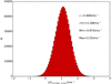 |
Fig. 8. Distribution of the radial velocity difference between SL 538 and NGC2006 obtained by direct cross-correlation of their bootstrapped spectra (see Sect. 4.3) for details). |
4.4 Relative flux comparison
In the following we describe how besides comparing the star-cluster radial velocities, we investigated the differences in the stellar population contents based on selected, strong spectral absorption features. We compared the two integrated spectra by subtracting them from one another and analyzing the residuals (see Fig. 5). Despite the fact that during the correction and combination of the individual orders we activated the flux conservation option in the IRAF package, we pay particular attention to the echelle order overlap regions, which are shown in Fig. 5 by vertical red stripes. Since the data reduction process was done identically for the two spectra, each one of them is affected by the same systematics. Therefore, by dividing (or subtracting) one by (or from) the other, the systematics do not affect our comparison as each spectrum follows the corresponding transmission curves of each order identically. Because of the obtained moderate data quality (peak S/N ≃ 13.6 for NGC2006 and ∼10.7 for SL 538), we decided not to fit stellar population model predictions to our spectra, but to compare qualitatively the shape of the absorption features from Table 1 for indications of different abundances.
The comparison was done in the following way: for each cluster we bootstrap the spectrum according to its variance spectrum, (i.e., adding noise in the same way as for the radial velocity uncertainty assessments; see previous sections). Then, we normalize the bootstrapped orders and finally subtract and divide the normalized fluxes of each cluster for a direct comparison. The results are presented in Fig. B.1 and show that there are significant differences in the line strengths of helium and the Balmer series between NGC2006 and SL 538. In the case of hydrogen, the NGC2006 spectrum shows stronger Balmer absorption, while the residuals are very symmetric for each of those absorption features. This is in line with the expectations from the CMD ages found for NGC2006 of 22.5–25 Myr, with SL 538 being ∼5 Myr younger. However, the helium lines show indications of substructure in the difference and flux-ratio spectra (see Fig. B.1), possibly hinting at different radial velocity distributions of stars (including stellar rotation velocity distribution profiles, stellar rotation axis alignments, and stellar mass segregation amongst others), which contribute mostly to these features with atmospheres typically hotter than those of B-type stars. We require higher S/N spectra to investigate the details of this intriguing difference in the absorption profiles of the various element species between these two star clusters.
4.5 Stellar population ages
In an attempt to constrain ages and to compare our observations with the predictions, and to roughly estimate metallicities with the aim to explore the differences (or similarities) that may hint the possible formation scenario and to compare our work with previous measurements, we have used high-resolution spectral energy distribution (SED) models from Starburst99 (v7.0.1 Leitherer et al. 1999, 2010, 2014; Vázquez & Leitherer 2005). Each normalized cluster SED was compared against theoretical SEDs (also normalized) with ages spanning from 5 Myr up to 40 Myr with intermediate steps of 1 Myr, considering the following metallicities: Z = 0.001, 0.008, 0.02, and 0.04 dex. We used the spectral region between 3750 Å and 5000 Å, avoiding the orders with the highest noise.
Results are presented in Fig. 9 where we show the χ2 as function of age for various metallicities. Residuals were visually inspected and we found that the absorption lines were not well reproduced by SEDs of 5 Myr. For the case of Z = 0.008 metallicity, absorption lines were best fitted (within the noise of the data) by SEDs with ages in the range ∼13 – 21 Myr with the formal absolute χ2-minimum at 14 Myr. The best-fit SED and residuals are shown in Figure 10. Due to the limited S/N of our data we were not able to further constrain the ages and metallicities of both clusters. Despite the formal minimum χ2 favoring an age of 14 Myr, we consider that the stellar population ages of both clusters fall in a range between 13 and 21 Myr for a metallicity near Z = 0.008, with a potential indication for the existence of very young (5 Myr old) stars. We point out that this is consistent with the results from Dieball & Grebel (1998).
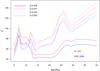 |
Fig. 9. χ2 as a function of stellar population age for a comparison between STARBURTS99 SEDs and the integrated spectra of NGC2006 (blue) and SL 538 (red). Various lines types encode the SED metallicity with values for Z = 0.001, 0.008, 0.02, and 0.04 as explained in the top-left legend. The absolute minimum is located for both clusters at 14 Myr for a metallicity of Z = 0.008, however, from the shape of the χ2 curve, the minimum is likely in the region between 14 and 21 Myr. |
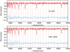 |
Fig. 10. Best fit with the observed spectra. Normalized observed spectrum is shown in gray, the red line corresponds to the Starburst99 14 Myr (for both clusters) model with a metallicity of Z = 0.008, and in light blue the residual (i.e., spectra subtracted by the model) is shown. Red stripes corresponds to the limits of the individual Echelle orders. |
5. Discussion
5.1 Cluster binarity
Measuring radial velocities on individual absorption features and the full spectrum gives us an idea of the robustness and stability of our measurements. Depending on the S/N of the spectrum at a given wavelength, we observe that the radial velocity values become more dispersed for blue features than for red ones. We also note that the radial velocities measured with the two techniques are more consistent for SL 538 than for NGC2006, which is likely due to the noise level of each individual profiles and their wider profile shapes.
For the following calculations we use the integrated-light measurements from the SIMBAD database2 , which give V = 10.88 mag for NGC2006 and V = 11.30 mag for SL 538, and assume a distance modulus of (m – M) = 18.493 (Pietrzyński et al. 2013) to both clusters and an absolute V-band solar luminosity of MV⊙ = 4.82 mag. We estimate a luminosity of LV = 9.3 × 10⁴ L⊙ for NGC2006 and LV = 6.9 × 10⁴ L⊙ for SL 538. If we adopt a mass-to-light ration of M/LV = 0.064 for a simple stellar population of 30 Myr (youngest age available in the model) and a metallicity Z = 0.008 with solar-scaled chemical composition from the BaSTI database3 , this yields a total stellar mass of Mcl = 5.9 × 10³ M⊙ for NGC 2006 and 4.3 × 10³ M⊙ for SL 538.
If we assume a circular orbit and a statistical proxy of the de-projected three-dimensional distance  , where RP is the projected distance (RP = 13.3 pc), the orbital period in years is then:
  , which yields Porb ≃ 60Myr. Therefore, the orbital velocity on a circular orbit can be computed as νorb = 2πR3D/Porb, which results in νorb = 1.66 km s−1. A similar result is obtained if values from Table 1 from Fujimoto & Kumai (1997) are taken into account. We point out that this value corresponds to the maximum observable velocity difference between the two clusters, but can change if elliptical orbits are invoked. In any case, the computed value agrees with our observed radial velocity difference of a few km s−1. Based on this estimate and similar, observed radial velocity differences in other cluster pairs, numerical simulations of the dynamical evolution of such star-cluster complexes (e.g., Yu et al. 2017; Grudić et al. 2018) suggest that these cluster pairs will merger within a few Myr. Based on their numerical simulations, Brüns et al. (2011) find that about half of the star cluster in their hierarchical complexes have merged after 2.5 crossing times, i.e., 2.5tcr. For our binary system we obtain
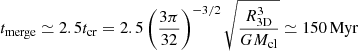
using the values for R3D and the total mass of the binary cluster (104 M⊙). Together these results argue in favor of the scenario in which such clusters are gravitationally bound entities, meaning that true binary star clusters that will merge within a few orbital timescales. However, we recall that absorption features are not identical in both clusters (see Sect. 4.3), which suggests a slightly different chemical abundance composition, at least in the case of helium. This may suggest a non-negligible variance and/or non-isotropy during the clusters’ (self-)enrichment process.
5.2 Formation scenario
Theoretical work from Fujimoto & Kumai (1997) advocates that the formation of binary star clusters may be a result of oblique cloud–cloud collisions that give rise to cloud fragmentation (i.e., Jeans gas clumps) and produce two or more gravitationally bound star clusters of roughly the same age in orbit with each other. This is, for example, believed to be the case in the binary cluster system NGC 2136/2137 (Mucciarelli et al. 2012). A different scenario has been proposed by Leon et al. (1999) where binary star clusters are born in rather separate environments, and form later by tidal capture, which would imply the presence of binary star clusters with significant age differences of their constituent stellar populations or a synchronized star-burst episode on spatial scales larger than individual proto-cluster complexes if no such age differences are measured. The derived CMD ages for our target clusters NGC 2006/SL 538 measured by Kumar et al. (2008), Dieball & Grebel (1998) and the similar ages derived from SED in our work show that overall an age difference between the two clusters is of the order of ≲5 Myr. Together with derived dynamical properties and the direct comparison of absorption line profiles of different elements showing some interesting residuals, which can be interpreted as a difference in internal chemical composition of each cluster, we tend to favor a scenario in which the origin of the NGC 2006/SL 538 pair is situated in a loosely bound star-formation complex that later on becomes a binary star cluster through tidal capture (see e.g., Grudić et al. 2018). Because of their similar masses and given the current separation and dynamics, this cluster pair is expected to merge within ∼150 Myr to form an open-cluster equivalent of approximately 104 M⊙ that will dissolve over the next few Gyrs.
6. Conclusions
The analysis of the derived velocity differences of the star cluster pair NGC 2006/SL 538 presented in this study are consistent with the expected orbital velocity of a gravitationally bound binary star cluster pair that will merge with the next ∼150 Myr. Cluster ages were constrained through full-SED fitting, but due to the low signal to noise, determined to lie in a range between 13 and 21 Myr for both clusters. When the normalized, integrated-light spectra are compared, we see some differences from helium in the residuals of their absorption features, which may be interpreted as differences in their chemical composition, concluding that this is likely a binary cluster that formed via tidal capture within a loosely bound star- formation complex rather than fragmentation of the same parent gas cloud.
Available at https://github.com/mmorage/LCO_ECHELLE
Acknowledgments
We thank the anonymous referee for his/her comments that help us to improve this paper. M. D. Mora is supported by CONICYT, Programa de astronomía, Fondo GEMINI, posición Postoctoral. THP acknowledges support through a FONDECYT Regular Project Grant (No. 1161817) and the support from CONICYT project Basal AFB-170002.
References
- Bellazzini, M., Ibata, R. A., Chapman, S. C., et al. 2008, AJ, 136, 1147 [NASA ADS] [CrossRef] [Google Scholar]
- Bhatia, R. K., & Hatzidimitriou, D. 1988, MNRAS, 230, 215 [NASA ADS] [Google Scholar]
- Bhatia, R. K., Read, M. A., Hatzidimitriou, D., & Tritton, S. 1991, A&AS, 87, 335 [NASA ADS] [Google Scholar]
- Brüns, R. C., Kroupa, P., Fellhauer, M., Metz, M., & Assmann, P. 2011, A&A, 529, A138 [NASA ADS] [CrossRef] [EDP Sciences] [Google Scholar]
- Coelho, P. R. T. 2014, MNRAS, 440, 1027 [NASA ADS] [CrossRef] [Google Scholar]
- De Silva, G. M., Carraro, G., D’Orazi, V., et al. 2015, MNRAS, 453, 106 [NASA ADS] [CrossRef] [Google Scholar]
- Dieball, A., & Grebel, E. K. 1998, A&A, 339, 773 [NASA ADS] [Google Scholar]
- Dieball, A., & Grebel, E. K. 2000, A&A, 358, 897 [NASA ADS] [Google Scholar]
- Dieball, A., Müller, H., & Grebel, E. K. 2002, A&A, 391, 547 [NASA ADS] [CrossRef] [EDP Sciences] [Google Scholar]
- Dirsch, B., Richtler, T., Gieren, W. P., & Hilker, M. 2000, A&A, 360, 133 [NASA ADS] [Google Scholar]
- Fellhauer, M., & Kroupa, P. 2005, MNRAS, 359, 223 [NASA ADS] [CrossRef] [Google Scholar]
- Fujimoto, M., & Kumai, Y. 1997, AJ, 113, 249 [NASA ADS] [CrossRef] [Google Scholar]
- Gratton, R. G., Carretta, E., & Bragaglia, A. 2012, A&ARv, 20, 50 [CrossRef] [Google Scholar]
- Grudić, M. Y., Guszejnov, D., Hopkins, P. F., et al. 2018, MNRAS, 481, 688 [NASA ADS] [CrossRef] [Google Scholar]
- Hatzidimitriou, D., & Bhatia, R. K. 1990, A&A, 230, 11 [NASA ADS] [Google Scholar]
- Hilker, M., Richtler, T., & Stein, D. 1995, A&A, 299, L37 [NASA ADS] [Google Scholar]
- Kontizas, E., Kontizas, M., & Michalitsianos, A. 1993, A&A, 267, 59 [NASA ADS] [Google Scholar]
- Kroupa, P. 1998, MNRAS, 300, 200 [NASA ADS] [CrossRef] [Google Scholar]
- Kumar, B., Sagar, R., & Melnick, J. 2008, MNRAS, 386, 1380 [NASA ADS] [CrossRef] [Google Scholar]
- Leitherer, C., Schaerer, D., Goldader, J. D., et al. 1999, ApJS, 123, 3 [NASA ADS] [CrossRef] [Google Scholar]
- Leitherer, C., Ortiz Otálvaro, P. A., Bresolin, F., et al. 2010, ApJS, 189, 309 [NASA ADS] [CrossRef] [Google Scholar]
- Leitherer, C., Ekström, S., Meynet, G., et al. 2014, ApJS, 212, 14 [NASA ADS] [CrossRef] [Google Scholar]
- Leon, S., Bergond, G., & Vallenari, A. 1999, A&A, 344, 450 [NASA ADS] [Google Scholar]
- Minniti, D., Rejkuba, M., Funes, J. G., & Kennicutt, Jr., R. C. 2004, ApJ, 612, 215 [NASA ADS] [CrossRef] [Google Scholar]
- Mucciarelli, A., Origlia, L., Ferraro, F. R., Bellazzini, M., & Lanzoni, B. 2012, ApJ, 746, L19 [NASA ADS] [CrossRef] [Google Scholar]
- Pietrzynski, G., & Udalski, A. 1999, Acta Astron., 49, 165 [NASA ADS] [Google Scholar]
- Pietrzyński, G., Graczyk, D., Gieren, W., et al. 2013, Nature, 495, 76 [NASA ADS] [CrossRef] [PubMed] [Google Scholar]
- Portegies Zwart, S. F., & Rusli, S. P. 2007, MNRAS, 374, 931 [NASA ADS] [CrossRef] [Google Scholar]
- Sugimoto, D., & Makino, J. 1989, PASJ, 41, 1117 [NASA ADS] [Google Scholar]
- Tonry, J., & Davis, M. 1979, AJ, 84, 1511 [NASA ADS] [CrossRef] [Google Scholar]
- van der Marel, R. P., Alves, D. R., Hardy, E., & Suntzeff, N. B. 2002, AJ, 124, 2639 [NASA ADS] [CrossRef] [Google Scholar]
- van Dokkum, P. G. 2001, PASP, 113, 1420 [NASA ADS] [CrossRef] [Google Scholar]
- Vázquez, G. A., & Leitherer, C. 2005, ApJ, 621, 695 [NASA ADS] [CrossRef] [Google Scholar]
- Yu, J., Puzia, T. H., Lin, C., & Zhang, Y. 2017, ApJ, 840, 91 [NASA ADS] [CrossRef] [Google Scholar]
Appendix A: Absorption profile fits
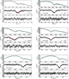 |
Fig. A.1. Absorption line profile fits for all features listed in Table 1. Features for the NGC 2006 spectrum are shown in the left panels, while the corresponding fits for SL 538 are given in the right panels. Each plot has three subpanels. Upper subpanel: observed spectrum near the absorption feature, where the cyan curve is the polynomial approximation to the continuum. Central subpanel: corresponds to the spectrum with the continuum subtracted, in which the black curve illustrates the Voigt profile fit, while the gray shadow represents the expected uncertainties from our bootstrapped experiments (see Sect. 4.2). The red curves in the central subpanel correspond to the bootstrapped 1σ uncertainty of the profile fit. Lower subpanels: residuals with their after continuum and profile subtraction together with their 1σ uncertainties as gray shadows. This figure shows profile fits for Balmer absorption features H10, Hη and Hϵ. |
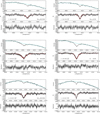 |
Fig. A.1. continued. Profile fits for the absorption features He I (4009.256Å), Hδ, and He I (4143.761Å). |
 |
Fig. A.1. continued. Profile fits for the absorption features Hγ, He I (4387.929Å), and Hβ. |
Appendix B: Absorption feature comparisons
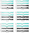 |
Fig. B.1. Absorption features comparison for H10, Hη, Hϵ, He I (4009.256Å), Hδ, and He I (4143.761Å). Each pair of spectra has been bootstrapped and radial-velocity corrected to be in the same rest-frame. The top panel of each figure shows the absorption feature spectrum portion for NGC 2006, while the lower panel shows the corresponding section for SL 538; the next panel below shows the normalized flux difference spectrum (NGC 2006–SL 538) and the bottom panel illustrates the flux ratio spectrum (NGC 2006/SL 538). The increasing noise seen on the right in some of the panels corresponds to the decreasing S/N of the spectra. |
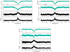 |
Fig. B.1. continued. Profile comparison for Hγ, He I (4387.929Å), and Hβ. |
All Tables
Summary of the radial velocity measurements from individual absorption features in NGC 2006 and SL 538.
All Figures
|
Fig. 1. Overview of the Large Magellanic Cloud (LMC) and the location, environment and morphology of the NGC 2006 (SL 539) and SL 538 star cluster pair. The figures are based on DSS colored images. Left panel: an overview of the LMC with the location of NGC 2006/SL 539 indicated by the arrow. The dashed square shows the outline of the zoom-in image in the top right panel, which illustrates the environment of the double star cluster. Bottom right panel: star cluster pair, separated by ∼13pc, within the stellar field of the immediate environment. |
| In the text | |
|
Fig. 2. Example of an arc frame from the MIKE spectrograph. We note that individual orders are heavily curved, as is typical for echelle spectra, in addition to a substantial tilt of the emission lines within each order that changes as a function of wavelength. |
| In the text | |
|
Fig. 3. Cut along the y-axis of the “pure-edge” image. Edge borders are indicated by positive count values and show a characteristic change in order width as a function of y-coordinate pixels, which corresponds to the spatial direction along the slit. |
| In the text | |
|
Fig. 4. Example of the order rectification and wavelength calibration correction. Top panel: rectified order cutout of an arc frame, not wavelength calibrated. Bottom panel: wavelength calibrated arc frame. |
| In the text | |
|
Fig. 5. Normalized integrated-light spectra for NGC 2006 ( top panel) and SL 538 ( middle panel). Bottom panel: difference spectrum (SL 538–NGC 2006). The vertical red lines in each panel mark the echelle order overlap regions. Some strong absorption features are labeled. |
| In the text | |
|
Fig. 6. Distribution of derived radial velocities from cross-correlation of the two target clusters and 1872 synthetic stellar template spectra from Coelho (2014). We note the differences in the asymmetric distributions of the resulting radial velocities, which indicates the degree of template mismatch for each cluster-template spectrum combination. |
| In the text | |
|
Fig. 7. Estimated radial velocity distributions for SL 538 ( top panel) and NGC2006 ( bottom panel) from cross-correlation of the bootstrapped cluster and the best-template stellar library spectra (see Sect. 4.3 for details). |
| In the text | |
|
Fig. 8. Distribution of the radial velocity difference between SL 538 and NGC2006 obtained by direct cross-correlation of their bootstrapped spectra (see Sect. 4.3) for details). |
| In the text | |
|
Fig. 9. χ2 as a function of stellar population age for a comparison between STARBURTS99 SEDs and the integrated spectra of NGC2006 (blue) and SL 538 (red). Various lines types encode the SED metallicity with values for Z = 0.001, 0.008, 0.02, and 0.04 as explained in the top-left legend. The absolute minimum is located for both clusters at 14 Myr for a metallicity of Z = 0.008, however, from the shape of the χ2 curve, the minimum is likely in the region between 14 and 21 Myr. |
| In the text | |
|
Fig. 10. Best fit with the observed spectra. Normalized observed spectrum is shown in gray, the red line corresponds to the Starburst99 14 Myr (for both clusters) model with a metallicity of Z = 0.008, and in light blue the residual (i.e., spectra subtracted by the model) is shown. Red stripes corresponds to the limits of the individual Echelle orders. |
| In the text | |
|
Fig. A.1. Absorption line profile fits for all features listed in Table 1. Features for the NGC 2006 spectrum are shown in the left panels, while the corresponding fits for SL 538 are given in the right panels. Each plot has three subpanels. Upper subpanel: observed spectrum near the absorption feature, where the cyan curve is the polynomial approximation to the continuum. Central subpanel: corresponds to the spectrum with the continuum subtracted, in which the black curve illustrates the Voigt profile fit, while the gray shadow represents the expected uncertainties from our bootstrapped experiments (see Sect. 4.2). The red curves in the central subpanel correspond to the bootstrapped 1σ uncertainty of the profile fit. Lower subpanels: residuals with their after continuum and profile subtraction together with their 1σ uncertainties as gray shadows. This figure shows profile fits for Balmer absorption features H10, Hη and Hϵ. |
| In the text | |
|
Fig. A.1. continued. Profile fits for the absorption features He I (4009.256Å), Hδ, and He I (4143.761Å). |
| In the text | |
|
Fig. A.1. continued. Profile fits for the absorption features Hγ, He I (4387.929Å), and Hβ. |
| In the text | |
|
Fig. B.1. Absorption features comparison for H10, Hη, Hϵ, He I (4009.256Å), Hδ, and He I (4143.761Å). Each pair of spectra has been bootstrapped and radial-velocity corrected to be in the same rest-frame. The top panel of each figure shows the absorption feature spectrum portion for NGC 2006, while the lower panel shows the corresponding section for SL 538; the next panel below shows the normalized flux difference spectrum (NGC 2006–SL 538) and the bottom panel illustrates the flux ratio spectrum (NGC 2006/SL 538). The increasing noise seen on the right in some of the panels corresponds to the decreasing S/N of the spectra. |
| In the text | |
|
Fig. B.1. continued. Profile comparison for Hγ, He I (4387.929Å), and Hβ. |
| In the text | |
Current usage metrics show cumulative count of Article Views (full-text article views including HTML views, PDF and ePub downloads, according to the available data) and Abstracts Views on Vision4Press platform.
Data correspond to usage on the plateform after 2015. The current usage metrics is available 48-96 hours after online publication and is updated daily on week days.
Initial download of the metrics may take a while.