| Issue |
A&A
Volume 622, February 2019
LOFAR Surveys: a new window on the Universe
|
|
|---|---|---|
| Article Number | A14 | |
| Number of page(s) | 10 | |
| Section | Extragalactic astronomy | |
| DOI | https://doi.org/10.1051/0004-6361/201833937 | |
| Published online | 19 February 2019 | |
Blazars in the LOFAR Two-Metre Sky Survey first data release
1
School of Physics, University College Dublin, Belfield Dublin 4, Ireland
e-mail: This email address is being protected from spambots. You need JavaScript enabled to view it.
2
ASTRON, Netherlands Institute for Radio Astronomy, PostBus 2, 7990 AA Dwingeloo, The Netherlands
3
Kapteyn Astronomical Institute, University of Groningen, PO Box 800, 9700 AV Groningen, The Netherlands
4
Leiden Observatory, Leiden University, PO Box 9513, 2300 RA Leiden, The Netherlands
5
Astrophysics, University of Oxford, Denys Wilkinson Building, Keble Road, Oxford OX1 3RH, UK
6
SUPA, Institute for Astronomy, Royal Observatory, Blackford Hill, Edinburgh EH9 3HJ, UK
7
CSIRO Astronomy and Space Science, PO Box 1130 Bentley WA 6102, Australia
8
Centre for Astrophysics Research, School of Physics, Astronomy and Mathematics, University of Hertfordshire, College Lane, Hatfield AL10 9AB, UK
9
INAF – Istituto di Radioastronomia, Via P. Gobetti 101, 40129 Bologna, Italy
10
Anton Pannekoek Institute for Astronomy, University of Amsterdam, Postbus 94249 1090 GE Amsterdam, The Netherlands
11
GEPI & USN, Observatoire de Paris, Université PSL, CNRS, 5 Place Jules Janssen, 92190 Meudon, France
12
Department of Physics & Electronics, Rhodes University, PO Box 94, Grahamstown 6140, South Africa
Received:
24
July
2018
Accepted:
18
October
2018
Abstract
Historically, the blazar population has been poorly understood at low frequencies because survey sensitivity and angular resolution limitations have made it difficult to identify megahertz counterparts. We used the LOFAR Two-Metre Sky Survey (LoTSS) first data release value-added catalogue (LDR1) to study blazars in the low-frequency regime with unprecedented sensitivity and resolution. We identified radio counterparts to all 98 known sources from the Third Fermi-LAT Point Source Catalogue (3FGL) or Roma-BZCAT Multi-frequency Catalogue of Blazars (5th edition) that fall within the LDR1 footprint. Only the 3FGL unidentified γ-ray sources (UGS) could not be firmly associated with an LDR1 source; this was due to source confusion. We examined the redshift and radio luminosity distributions of our sample, finding flat-spectrum radio quasars (FSRQs) to be more distant and more luminous than BL Lacertae objects (BL Lacs) on average. Blazars are known to have flat spectra in the gigahertz regime but we found this to extend down to 144 MHz, where the radio spectral index, α, of our sample is −0.17 ± 0.14. For BL Lacs, α = −0.13 ± 0.16 and for FSRQs, α = −0.15 ± 0.17. We also investigated the radio-to-γ-ray connection for the 30 γ-ray-detected sources in our sample. We find Pearson’s correlation coefficient is 0.45 (p = 0.069). This tentative correlation and the flatness of the spectral index suggest that the beamed core emission contributes to the low-frequency flux density. We compare our sample distribution with that of the full LDR1 on colour-colour diagrams, and we use this information to identify possible radio counterparts to two of the four UGS within the LDR1 field. We will refine our results as LoTSS continues.
Key words: surveys / radiation mechanisms: general / radio continuum: galaxies / gamma rays: galaxies / galaxies: active / BL Lacertae objects: general
© ESO 2019
1. Introduction
The centres of some galaxies are extremely luminous, producing broadband non-thermal emission. These compact regions are known as active galactic nuclei (AGN). Some fraction of AGN are understood to have relativistic jets and by chance some of the jets are orientated close to our line of sight. Such AGN are known as blazars (see the review by Urry & Padovani 1995). The jets are believed to be powered by the accretion of matter onto supermassive black holes residing at the galactic cores. Relativistic beaming effects give rise to apparent superluminal motion, and Doppler boosting increases the observed luminosity. Although blazars are the most common sources in the γ-ray regime (Acero et al. 2015), only a small number of blazars are γ-ray-loud and the reasons for this are still unclear (Fan et al. 2012).
There are two types of blazars that are distinguished by their observational properties: BL Lacertae objects (BL Lacs) and flat-spectrum radio quasars (FSRQs). The populations are defined by the presence or absence of strong emission lines, which is controlled by the inner accretion disc. BL Lacs possess featureless optical spectra and are generally associated with beamed jet-mode (radiatively inefficient) AGN. In contrast, strong optical emission lines are a characteristic of FSRQs and they are often associated with beamed radiative-mode AGN. However, one commonality shared by BL Lacs and FSRQs is the broadband nature of the radiation they emit.
The characteristic structure seen in the spectral energy distributions (SEDs) for blazars consists of two components in the νFν–ν plane (where ν is frequency and Fν is flux), which has the non-thermal components dominating energetically over the thermal component at all wavelengths. These two components give the blazar SEDs their characteristic double-humped shape.
The first component begins in the radio waveband and peaks in the optical or X-ray waveband. This emission can be attributed to synchrotron processes from a population of relativistic (≳keV) electrons in a magnetic field. Blazars typically possess flat spectra at gigahertz frequencies, where the radio spectral index, α, is defined as S(ν) ∝ να, typically α > −0.5. Nori et al. (2014) found that blazars have flat spectra down to ∼300 MHz. At lower frequencies, the spectrum becomes inverted (i.e. α > 0) because of synchrotron self-absorption.
The second feature of the SED peaks between the MeV and TeV energy bands and may be caused by inverse-Compton scattering (e.g. Sikora et al. 1994) but this remains an open question (Beckmann & Shrader 2012). If this is the case, then seed photons originating from the synchrotron process are inverse-Compton scattered by the electrons in the jet to higher energies (i.e. synchrotron self-Compton radiation; Marscher & Gear 1985). However, it is also possible that the seed photons originate from outside the jet – for example, from the accretion disc or broad line region. Alternatively, the high-energy peak of the SED may be the result of hadronic synchrotron processes, rather than leptonic inverse-Compton processes (Böttcher 2007).
We search for a correlation between the low-frequency radio emission and the γ-ray emission in this study. The existence of such a correlation is still debated (Pavlidou et al. 2012). Several studies have found a correlation (Stecker et al. 1993; Padovani et al. 1993; Salamon & Stecker 1994; Ackermann et al. 2011; Linford et al. 2012). However, taking all biases into account, such as the limited dynamic range (when considering flux densities) or the common redshift dependence (when considering luminosities) is non-trivial (Kovalev et al. 2009). For example, Mücke et al. (1997) and Chiang & Mukherjee (1998) disputed evidence of a correlation on the grounds of redshift biases and the sensitivity limits of the surveys used.
Studying blazars at megahertz frequencies is challenging because their characteristic flat spectra make it difficult to identify counterparts in this regime. For example, Giroletti et al. (2016) used the Murchison Widefield Array Commissioning Survey (MWACS; Hurley-Walker et al. 2014) to examine the 120–180 MHz emission from blazars. The MWACS has ∼3′ angular resolution and a typical noise level of 40 mJy beam−1, which allowed Giroletti et al. (2016) to identify low-frequency counterparts to 186 of 517 (36%) blazars in the MWACS footprint. Giroletti et al. (2016) then calculated the mean low-frequency spectral index to be −0.57 ± 0.02, and identified a mild correlation between the radio flux density and the γ-ray energy flux (r = 0.29, p = 0.061). Callingham et al. (2017) also identified a small number of blazars that show a peaked spectrum in the low-frequency spectra from the GLEAM survey (Hurley-Walker et al. 2017). This emphasises that a simple selection of flat-spectrum radio sources may not select all blazars. However, both Callingham et al. (2017) and Giroletti et al. (2016) were limited in their resolution and sensitivity to explore the population in depth.
We use the LOFAR Two-Metre Sky Survey (LoTSS) first data release value-added catalogue (LDR1) to study the 144 MHz properties of blazars (Shimwell et al. 2019; Williams et al. 2019; Duncan et al. 2019). We cross-matched LDR1 with the Third Fermi-LAT Point Source Catalogue (3FGL; Acero et al. 2015), the Roma-BZCAT Multi-frequency Catalogue of Blazars (5th edition; Massaro et al. 2015), and the very-high-energy catalogue called TeVCAT (Wakely & Horan 2008). The LDR1 catalogue covers 424 deg2 of the sky with future data releases aiming to significantly expand this to full coverage of the northern sky. In this respect, this work paves the way for a larger study with future data releases.
This paper is organised as follows: The sample of sources used for this study was constructed from several surveys and catalogues, each of which is described in turn in Sect. 2. The way in which we built our sample is detailed in Sect. 3. Our results are presented in Sect. 4 and discussed in Sect. 5. We use a ΛCDM cosmological model throughout this paper with h = 0.71, Ωm = 0.26, and ΩΛ = 0.74, where H0 = 100h km s−1 Mpc−1 is the Hubble constant. We maintain the definition of α, where S(ν)∝να.
2. Surveys and catalogues
2.1. LOFAR Two-Metre Sky Survey first data release
The LOw Frequency ARray (LOFAR) is a radio interferometer with stations located throughout Europe (van Haarlem et al. 2013). The LOFAR Surveys key science project aims to map the sky above the northern hemisphere between 120 MHz and 168 MHz. A full description of the LoTSS can be found in Shimwell et al. (2017). The LoTSS is underway, making use of the core and remote LOFAR stations in the Netherlands.
The first data release is outlined in Shimwell et al. (2019) and the value-added catalogue is outlined in Williams et al. (2019) and Duncan et al. (2019). The LDR1 uses data collected between 2014 May 23 and 2015 October 15, focussing on the HETDEX Spring Field (Hill et al. 2008). The right ascension ranges approximately from 10 h 45 m 00 s to 15 h 30 m 00 s and the declination ranges approximately from 45° 00′ 00″ to 57° 00′ 00″; the advantage of this region for the study of blazars is that it is far from the galactic centre. Furthermore, the 6″ angular resolution and 71 μJy beam−1 median sensitivity of LDR1 is unrivaled with respect to existing radio surveys. To study the blazar population, we use this catalogue described in Shimwell et al. (2019), which has the direction-dependent corrections applied.
2.2. 3FGL and 3LAC
The 3FGL is based on data from the first four years of Fermi-LAT, covering the 0.1–300 GeV energy range (Acero et al. 2015). There are 3 033 sources in 3FGL, of which 1 009 are unassociated γ-ray sources (UGS). These are sources to which a known source could not be unambiguously linked, often due to source confusion.
The Third Catalogue of AGN detected by Fermi-LAT (3LAC) is the most comprehensive catalogue of γ-ray AGN at present. The 3LAC is based on 3FGL sources that have a test statistic >25 (i.e. ≳5σ significance) between 100 MeV and 300 GeV over the period extending from 2008 August 04 to 2012 July 31 (Ackermann et al. 2015). The 3LAC contains 1 773 AGN in total with 491 (28%) FSRQs, 662 (37%) BL Lacs, 585 (33%) blazars of unknown type, and 35 (2%) sources of other types. We use the improved source positions and blazar classification information in 3LAC to aid in the study of our sample.
2.3. BZCAT
BZCAT is a catalogue of blazars that contains multi-frequency data from a number of surveys (Massaro et al. 2015). The BZCAT contains radio flux measurements which are either at 1.4 GHz from the National Radio Astronomy Observatory Very Large Array Sky Survey (NVSS; Condon et al. 1998) (0.45 mJy beam−1 sensitivity) or at 0.8 GHz from the Sydney University Molonglo Sky Survey (SUMSS). For the region of sky we are interested in, the radio flux measurements used are those at 1.4 GHz because sources in LDR1 have a declination >−30°. The source positions are mostly derived from very-long-baseline interferometry measurements. In addition, BZCAT reports information from the Wide-field Infrared Survey Explorer (WISE) and the Sloan Digital Sky Survey (SDSS) optical database.
Edition 5.0.0 of BZCAT was used and, while 3FGL contains a higher fraction of BL Lacs, BZCAT lists mostly FSRQs. Of the 3 561 sources in BZCAT, 1 909 (54%) are FSRQs, 1 425 (40%) are BL Lacs, 227 (6%) are blazars of uncertain type, and 274 (8%) are galaxy-dominated blazars.
2.4. TeVCAT
We searched for sources in TeVCAT (Wakely & Horan 2008), which provides TeV data, but found no sources within the LDR1 footprint. However, this will become an important source of information with which to study blazars as LoTSS progresses.
3. Analysis
3.1. Sample construction
For the high-energy sources, BZCAT positional data were used where available, and 3LAC data were used secondarily. Both have accurately defined positions. Likewise, the source classifications (FSRQs, BL Lacs, etc.) were taken from BZCAT in the first instance and from 3LAC for sources without a BZCAT association. For the UGS, 3FGL positions were used, which had comparatively large uncertainty ellipses.
Using TOPCAT (Tool for Operations on Catalogues and Tables; Taylor et al. 2005), we cross-matched the catalogues with LDR1, where the LDR1 positions take account of any extended features, not just the core regions. We implemented a 12″ search radius. Although this is comparatively large compared to the astrometric uncertainties (the average uncertainty on the position of an LDR1 source is ∼0.3″), 93% of LDR1 sources were unique matches within 7″ of the BZCAT or 3LAC positions. The seven sources with a separation of 7–12″ are extended in LDR1, and also had unique matches within 12″. All matches were confirmed visually and images showing the sources in our sample along with the BZCAT/3LAC positions can be found online1.
An overview of the 102 unique extragalactic sources in our sample is given in Table 1, where 68 sources were in BZCAT only and therefore have no γ-ray detection. An LDR1 match was found for all sources, excluding the UGS; a unique match could not be determined for the four UGS because of source confusion.
Breakdown of our sample according to catalogue and source type.
To investigate the likelihood of spurious detections, we shifted all sources in BZCAT by 2° in a random direction and performed the same cross-matching procedure as before. We repeated this several times and found no matches within 7″ and ∼2 matches within 10″, indicating that it is likely our sample is free from such spurious detections.
3.2. Radio spectral index
To calculate the radio spectral indices, flux density measurements from several surveys in the 0.07–1.4 GHz range were employed: the Very Large Array Low-frequency Sky Survey Redux (VLSSr; Lane et al. 2014), the 7th Cambridge Survey of Radio Sources (7C), the Westerbork Northern Sky Survey (WENSS; Rengelink et al. 1997), and NVSS were used where available. Table 2 shows the frequency corresponding to each survey and the number of sources for which each survey had data. The TIFR Giant Metrewave Radio Telescope Sky Survey First Alternative Data Release (TGSS ADR1; Intema et al. 2017) was not used in spectral fitting but is shown in Table 2 to allow for comparisons.
Number of sources found in each catalogue or survey.
The spectral modelling performed was identical to that done by Callingham et al. (2015). In summary, the Markov chain Monte Carlo (MCMC) algorithm emcee (Foreman-Mackey et al. 2013) was used to sample the posterior probability density functions of a power-law or a curved-power-law model (see Eqs. (1) and (2) of Callingham et al. 2017). Physically sensible priors were applied (such as that the normalisation constant cannot be negative) and a Gaussian likelihood function was maximised by applying the simplex algorithm to direct the walkers (Nelder & Mead 1965). For this method, the uncertainties reported on the flux density values in all the surveys were assumed to be Gaussian and independent.
We compared the modelled spectral index to the spectral index where only the lowest (VLSSr where available, but LDR1 in the majority of cases) and highest frequencies (NVSS) were used, αmin − max. We found αmin − max = −0.20 ± 0.14, and this is in agreement with α = −0.17 ± 0.14, when all points are used. The equation of the line between these quantities is αmin − max = 0.97α − 0.03, where r = 0.96, indicating that fitting a power law to the sources in our sample is a valid assumption.
The majority (83%) of our sources are found in both TGSS and NVSS and hence appear in the TGSS-to-NVSS spectral index catalogue (de Gasperin et al. 2018). These sources have an average TGSS-to-NVSS spectral index of −0.28 ± 0.15, which is in keeping with our result of α = −0.24 ± 0.14 for the same sample.
3.3. Blazar variability
Blazars can exhibit flux variability from radio to γ-ray energies (Richards et al. 2011), making it necessary to assess the impact of any inherent variability on the derived spectral indices and the strength of the radio-to-γ-ray correlation.
The surveys used to calculate the spectral index are non-simultaneous, so it is possible that the flux densities used to fit α change over time. However, there is less radio variability in blazars below the synchrotron peak than above it (Urry 1998). In support of this, Bell et al. (2018) found that blazars do not seem to be significantly variable at low frequencies and McGilchrist & Riley (1990) found little variability of 7C sources at 151 MHz. Pandey-Pommier et al. (2016) monitored PKS 2155-304, one of the brightest BL Lacs, while it was flaring and found only marginal variability at 235 MHz. Furthermore, Turriziani et al. (2015) conducted a preliminary blazar monitoring programme with LOFAR at 226 MHz, focussing on five blazars which exhibit strong gigahertz variability. The LOFAR light curves revealed a smooth behaviour (with some possible changes to the flux of the order of months). Hence, it is the NVSS flux densities which we expect to be most affected by variability, since this was the only catalogue we used >325 MHz. We included data from several megahertz surveys in the spectral modelling to minimise the influence of this possible variability, but the NVSS data are still the most influential when calculating α.
The LDR1 and 3FGL catalogues are non-contemporaneous: LDR1 observations were made between 2014 and 2015 while 3FGL observations were integrated between the years 2008 and 2012. As a result, for any blazars which exhibit strong γ-ray variability, the data in 3FGL correspond to an average value and are more indicative of the non-flaring state. Since we do not expect the 144 MHz or γ-ray data to be variable, we conclude that the non-simultaneity does not significantly impact any correlation between the radio and γ-ray bands.
4. Results
4.1. Detection rate and redshift
We identified LDR1 counterparts to 100% of the high-energy sources (excluding UGS) and a summary of our results are given in Table 3. Information on the individual 98 sources in our sample is presented in Table A.1 at the end of this paper. In our sample, 48% of sources are FSRQs, 25% are BL Lacs, 8% are blazars of uncertain type or BL Lac candidates, and 16% are other source types (e.g. galaxy-dominated blazars, AGN, radio galaxies, and UGS).
Summary of our results.
Most (77/98) redshifts are the spectroscopic LDR1 values. The remainder are from BZCAT (6/98), the NASA/IPAC Extragalactic Database (6/98), 3LAC (1/98), or are LDR1 photometric estimates (6/98); two sources have no measured redshift. Obtaining photometric redshifts for blazars is challenging owing to the lack of reliable SED templates, but the LDR1 photometric redshifts are dominated by machine learning estimates which do not depend on such templates. The caption of Table A.1 contains a link to the CSV version of the table, which shows the origin of z for each source.
Figure 1 shows the redshift distribution of our sample as well as the distributions of BZCAT and 3LAC. In BZCAT, 2 842 of the 3 561 sources have redshifts (see Fig. 1b), and in 3LAC, 896 of the 1 773 sources have a measured redshift (see Fig. 1c). The redshift distribution of our sample follows a similar trend to the BZCAT distribution, but in 3LAC there is a larger percentage of low-redshift BL Lacs. The FSRQ population is more distant than BL Lacs on average in all cases.
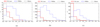 |
Fig. 1. Distribution of the measured redshift values in our sample (panel a) compared to BZCAT (panel b) and 3LAC (panel c). Included in “Others” are, for example, blazars of uncertain type, BL Lac candidates, and galaxy-dominated BL Lacs. |
4.2. Flux density and luminosity
The 144 MHz radio flux density, S144 MHz, in our sample ranges from 1.3 mJy to 14 Jy. The FSRQs have a higher median S144 MHz than the BL Lacs, as seen in Table 3. The median S144 MHz for γ-ray-detected sources (193 ± 105 mJy) and for non-γ-ray-detected sources (203 ± 19 mJy) are within error of each other.
We calculated the radio luminosity, Lν (in W Hz−1), according to
where S144 MHz is in W m−1 Hz−2 and d is the luminosity distance in metres. Figure 2 shows the distribution of Lν for our sample. The FSRQs span a broad range of Lν while the BL Lacs are predominantly in the lower bins, as expected.
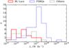 |
Fig. 2. Radio luminosity distribution for our sample is shown. |
4.3. Radio spectral index
Figure 3 shows the radio spectral index distribution, and the average values are given in Table 3. The average α for our sample is −0.17 ± 0.14, and this is much flatter than α for all sources in LDR1, which we expect to be −0.8 ≲ α ≲ −0.7. Our results suggest both BL Lacs and FSRQs are flat even at megahertz frequencies. We found α = −0.11 ± 0.17 for the γ-ray sources, which is similar to the non-γ-ray-detected blazars where α = −0.21 ± 0.16. Giroletti et al. (2016) found α = −0.57 ± 0.02, which is steeper than the α we calculated. This can be explained by the fact that all blazars in the field were detected in this study, whereas Giroletti et al. (2016) detected 36% of blazars. This introduces a selection effect against flat or inverted-spectrum sources.
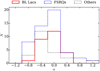 |
Fig. 3. Distribution of the radio spectral indices for the sources in our sample is shown. |
The contribution of the flat-spectrum core to the flux density is understood to decrease as the frequency decreases and, in the megahertz regime, the flux density is thought to be dominated by the extended emission in the radio lobes. However, the flatness of α suggests the beamed core emission is contributing somewhat to the low-frequency flux density. As our sample consists of blazars, Doppler boosting can lead to the core component appearing disproportionately brighter than the extended component.
The spectra for some sources in our sample appear to be gigahertz-peaked spectrum (GPS) sources (Callingham et al. 2017). An example is seen in Fig. 4, which shows the spectra from which α was derived for two sources in our sample. It has previously been argued that GPS quasars are flaring blazars (Tinti et al. 2005) or intrinsically young radio sources (Fanti et al. 1995).
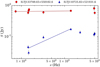 |
Fig. 4. Flat spectrum source and peaked spectrum source from our sample. The spectral fits we derived using data up to 1.4 GHz are shown as solid lines. Data from NED up to 5 GHz have been plotted. The flatness of the radio spectrum for ILTJ133749.65+550102.6 is clear, as is the GHz peak for ILTJ110725.82+521931.6. |
4.4. Radio–γ-ray connection
Figure 5 shows the radio flux density plotted against the γ-ray energy flux for the γ-ray-detected sources. The γ-ray energy flux at 100 MeV was calculated from the integrated photon flux given in 3FGL using the γ-ray power-law spectral index. Two sources not in the 3LAC “clean” sample and 3C 303 were excluded. A linear fit to the logarithms of the flux yields a slope, and hence power-law index, of m = 0.61 ± 0.25. We obtained a Pearson correlation coefficient, r, of 0.45 with a null-hypothesis p-value of 0.019. This marginally significant p-value is limited by our N = 27 sample size, and the sample sizes were too small to calculate the correlation with any meaningful significance for the BL Lac or FSRQ populations. This correlation also does not address the biases within the data.
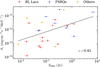 |
Fig. 5. γ-ray energy flux density is plotted against the radio flux density. A line was fit to the logarithms of the data. The radio flux density is at 144 MHz and the γ-ray energy flux density measurements correspond to 100 MeV. |
We then used the Monte Carlo correlation method outlined by Pavlidou et al. (2012) in our radio-to-γ-ray analysis, which has also been used by Ackermann et al. (2011). This method was designed for small samples affected by distance effects and subjective sample selection criteria. The data are randomised in luminosity space. This accounts for the fact that the radio and γ-ray flux densities appear to be correlated because of their common redshift. Then the significance is measured in flux space to avoid Malmquist bias (Lister & Marscher 1997).
The Pavlidou et al. method gave the r = 0.45 correlation a significance of p = 0.069. This is therefore suggestive of a correlation, although we cannot conclusively reject the null hypothesis that the radio and γ-ray luminosities of blazars are independent. Furthermore, this method provides a conservative estimate for small samples and so, while real correlations may not be verified, exaggerated significances are avoided in cases where there is insufficient evidence.
This correlation is weaker than the gigahertz radio-to-γ-ray connection for the same sample (r = 0.57, p = 0.002), as we would expect, given that the emission is usually more diffuse at lower frequencies.
4.5. Colour-colour diagrams
In 2010, WISE observed the sky at 3.4 μm (W1), 4.6 μm (W2), 12 μm (W3), and 22 μm (W4). These magnitudes are included in LDR1, from which we calculated the colours. Figure 6 shows the W1 − W2 − W3 colour-colour and colour-magnitude diagrams. Sources in our sample are plotted over the LDR1 catalogue, where LDR1 sources are predominantly star-forming galaxies. It is clear that blazars populate distinct regions compared to LDR1 on each of these plots, but the blazar population is the most compact in Fig 6a.
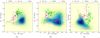 |
Fig. 6. Two-dimensional histograms show the W1 − W2 vs. W2 − W3 (panel a) and the W1 − W2 vs. W3 − W4 (panel b) colour-colour diagrams, and the W1 − W2 vs. W1 − W2 (panel c) colour-magnitude diagram. The IR colours for the entire LDR1 sample for which there is WISE data available (218 595 of 318 520 sources) is the two-dimensional histogram, with contours indicating the 25%, 50%, and 75% levels. The points are the LDR1 sources from our sample for which there is WISE data (96 of 98 sources). |
In Fig. 6a, the WISE blazar strip can be seen (Massaro et al. 2011). Generally, blazars are dominated by synchrotron emission in the infrared (IR) band. As a result, blazars have a distinct locus to that of the LDR1 sources, the majority of which of are dominated by a thermal component in the IR. The distribution of blazars in Fig. 6a is in agreement with a power-law model for the IR spectrum. Moreover, BL Lacs and FSRQs also inhabit distinct regions on this colour-colour diagram, and the locations of these populations are consistent with the findings of Massaro et al. (2011). Some blazars lie outside the blazar strip, and in this case, it is possible that there is a non-negligible thermal contribution to the IR emission from the host galaxy.
Figure 6b shows a different combination of IR colours, where the blazar population is also removed from the thermal LDR1 population. Figure 6c plots the W1 magnitude, which is the band with the highest sensitivity, against the W1 − W2 colour. The blazars appear brighter than LDR1 sources of the same colour as a result of Doppler boosting. The majority of blazars have W1 − W2 ≈ 1, as noted by D’Abrusco et al. (2012). This corresponds to an IR spectral index of −1 and suggests the synchrotron component peaks close to the WISE measurements. Furthermore, Stern et al. (2012) used W1 − W2 > 0.8 as criterion to select for AGN, as this distinguishes between the AGN power-law spectra and the galactic black-body spectra.
The four 3FGL UGS within the LDR1 footprint are shown in Table 4 alongside the number of LDR1 sources which fall within the 3FGL 95% ellipse. This is illustrated for 3FGL J1051.0+5332 in Fig. 7 where the semi-major and semi-minor axes are 0.213° and 0.155°, respectively. Colour information from WISE has previously been used to classify UGS by D’Abrusco et al. (2013). We also used the colour-colour diagrams to identify possible counterparts to the UGS on the basis that, statistically, these γ-ray sources are most likely to be blazars because blazars dominate the extragalactic γ-ray sky.
UGS within the LDR1 footprint, along with the number of LDR1 sources within the 95% uncertainty ellipse.
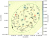 |
Fig. 7. Unassociated γ-ray source 3FGL J1051.0+5332 with 68% (yellow) and 95% (green) confidence ellipses is shown. Squares mark the LDR1 sources which lie within the 95% confidence band; the three red diamonds are the sources which we assess to be the most likely match. |
We chose 96 sources at random from LDR1 because colour information was available for 96 sources in our sample. We plotted these two populations on colour-colour diagrams (not shown) and used an inverse-distance-weighted k-nearest neighbours (k-NN) algorithm (where k = 3) to identify which UGS matches were likely to be blazars. From the total 282 possible LDR1 matches for the UGS, only four are likely to be blazars. Three matched with one source, one UGS had just a single possibility, and two UGS had no possible matches remaining. The properties of these potential matches are given in Table 5.
Likely matches to the UGS.
Advantages of this k-NN method are that it assumes no prior knowledge of the region inhabited by blazars in colour space and that the implementation is straightforward. Identifying two of four possible counterparts is a promising return and based on experience the resulting matches seem plausible, but we will be able to better quantify the success of this method as the LoTSS footprint increases. We will also be able to test the reliability of this method against other supervised (e.g. principal component analysis, as used by D’Abrusco et al. 2013) and unsupervised (e.g. k-means clustering) machine learning techniques. However, these algorithms can only successfully identify quintessential blazars and those for which WISE data are available. For the UGS in this study without a likely match, it is possible that the counterparts lie beyond the blazar strip, where the synchrotron radiation is not the dominant component at IR wavelengths.
5. Conclusions
We examined the radio properties of the high-energy sources from BZCAT and 3FGL within LDR1. Because of their broadband nature, studying how blazars behave at low frequencies is essential to understanding how they operate. Historically, studying the low-frequency properties of blazars as a population has proven difficult because it has not been possible to identify low-frequency radio counterparts to these high-energy sources with the limited angular resolution and sensitivity of ∼100 MHz surveys. The LDR1 catalogue addresses this technological gap and it is a marked improvement over even recent low-frequency surveys, such as MWACS and TGSS ADR1, in terms of angular resolution and sensitivity. As a result, we were able to find counterparts for all 3FGL and BZCAT sources in our field (excluding the UGS).
Despite their poorly-constrained γ-ray position and the density of sources in the LDR1 field, we were able to identify possible radio counterparts for two of the four UGS within the LDR1 footprint using the WISE colour information provided in the value-added catalogue. The radio spectral index was not available for most of the possible counterparts as the sources only had an LDR1 detection in the radio regime, but the availability of LoTSS in-band spectral indices in a future data release could help in matching these UGS.
The 100% detection rate of blazars in this study, alongside the wealth of ancillary information in the value-added catalogue makes the LoTSS first data release an extremely useful resource in studying the low-frequency properties of these high-energy sources. Indeed, preliminary efforts suggest that it may possible to use LDR1 to discover new blazars in the field, for follow up with other instruments. We looked to use this k-NN method to identify sources in LDR1 which are possibly blazars. From the 218 595 sources with four WISE colours, ∼1% fell within the blazar-populated space for all of the colour diagrams. This number could be cut down further by placing sensible limitations on the redshift and spectral index and this will be investigated in a future study.
In total, there are 1 444 3FGL sources and 2 138 BZCAT sources in the northern hemisphere sky, which is the final goal of LoTSS in terms of sky coverage. As LoTSS progresses, we plan to revisit this work and evaluate the properties of blazar subclasses. The inherent variability of blazars will be an ever-present issue because the different observational methods for the radio and γ-ray regimes means that acquiring perfectly contemporaneous observations is challenging. But a larger sample size means we will be able to deduce general trends with more confidence and this should reduce the influence of flaring blazars. It is fortunate that LoTSS comes at a time when Fermi is still operational because Fermi is unrivaled with respect to γ-ray detections. Weaker γ-ray sources will be present in 4FGL, the next Fermi-LAT catalogue which is due to be released in 2018. The radio counterparts of these sources will be fainter too, possibly with more high-frequency-peaked BL Lacs, and LoTSS will be a valuable resource when it comes to identifying these sources.
Acknowledgments
SM acknowledges support from the Irish Research Council Postgraduate Scholarship and the Irish Research Council New Foundations Award. RM gratefully acknowledges support from the European Research Council under the European Union’s Seventh Framework Programme (FP/2007-2013) /ERC Advanced Grant RADIOLIFE-320745. HR and KJD acknowledge support from the ERC Advanced Investigator programme NewClusters 321271. LKM acknowledges support from Oxford Hintze Centre for Astrophysical Surveys, which is funded through generous support from the Hintze Family Charitable Foundation. This publication arises from research partly funded by the John Fell Oxford University Press (OUP) Research Fund. PNB is grateful for support from the UK STFC via grant ST/M001229/1. GG acknowledges the CSIRO OCE Postdoctoral Fellowship. MJH acknowledges support from the UK Science and Technology Facilities Council [ST/M001008/1]. IP acknowledges support from INAF under PRIN SKA/CTA ‘FORECaST’. JS is grateful for support from the UK STFC via grant ST/M001229/1. WLW acknowledges support from the UK Science and Technology Facilities Council [ST/M001008/1]. This paper is based (in part) on data obtained with the International LOFAR Telescope (ILT) under project code s LC2_038 and LC3_008. LOFAR (van Haarlem et al. 2013) is the LOw Frequency ARray designed and constructed by ASTRON. It has observing, data processing, and data storage facilities in several countries, which are owned by various parties (each with their own funding sources), and are collectively operated by the ILT foundation under a joint scientific policy. The ILT resources have benefited from the following recent major funding sources: CNRS-INSU, Observatoire de Paris and Universitè d’Orlèans, France; BMBF, MIWF-NRW, MPG, Germany; Science Foundation Ireland (SFI), Department of Business, Enterprise and Innovation (DBEI), Ireland; NWO, The Netherlands; The Science and Technology Facilities Council, UK; Ministry of Science and Higher Education, Poland. Part of this work was carried out on the Dutch national e-infrastructure with the support of the SURF Cooperative through grant e-infra 160022 & 160152. The LOFAR software and dedicated reduction packages on https://github.com/apmechev/GRID_LRT were deployed on the e-infrastructure by the LOFAR e-infragroup, consisting of J. B. R. Oonk (ASTRON & Leiden Observatory), A. P. Mechev (Leiden Observatory) and T. Shimwell (ASTRON) with support from N. Danezi (SURFsara) and C. Schrijvers (SURFsara). This research has made use of data analysed using the University of Hertfordshire high-performance computing facility (http://uhhpc.herts.ac.uk/) and the LOFAR-UK computing facility located at the University of Hertfordshire and supported by STFC [ST/P000096/1]. This research has made use of the NASA/IPAC Extragalactic Database (NED), which is operated by the Jet Propulsion Laboratory, California Institute of Technology, under contract with the National Aeronautics and Space Administration. This research has made use of SciPy software (Jones et al. 2001) and Topcat (Taylor et al. 2005).
References
- Acero, F., Ackermann, M., Ajello, M., et al. 2015, ApJS, 218, 23 [Google Scholar]
- Ackermann, M., Ajello, M., Allafort, A., et al. 2011, ApJ, 741, 30 [NASA ADS] [CrossRef] [Google Scholar]
- Ackermann, M., Ajello, M., Atwood, W. B., et al. 2015, ApJ, 810, 14 [NASA ADS] [CrossRef] [Google Scholar]
- Beckmann, V., & Shrader, C. 2012, Proceedings of “An INTEGRAL view of the high-energy sky (the first 10 years)” - 9th INTEGRAL Workshop and celebration of the 10th anniversary of the launch, 69 [Google Scholar]
- Bell, M. E., Murphy, T., & Hancock, P. J. 2018, MNRAS, sty2801 [Google Scholar]
- Böttcher, M. 2007, Astrophys. Space Sci., 309, 95 [Google Scholar]
- Callingham, J. R., Ekers, R. D., Gaensler, B. M., et al. 2017, ApJ, 836, 174 [NASA ADS] [CrossRef] [Google Scholar]
- Callingham, J. R., Gaensler, B. M., Ekers, R. D., et al. 2015, ApJ, 809, 168 [NASA ADS] [CrossRef] [Google Scholar]
- Chiang, J., & Mukherjee, R. 1998, ApJ, 496, 752 [NASA ADS] [CrossRef] [Google Scholar]
- Condon, J. J., Cotton, W. D., Greisen, E. W., et al. 1998, AJ, 115, 1693 [NASA ADS] [CrossRef] [Google Scholar]
- D’Abrusco, R., Massaro, F., Ajello, M., et al. 2012, ApJ, 748, 68 [NASA ADS] [CrossRef] [Google Scholar]
- D’Abrusco, R., Massaro, F., Paggi, A., et al. 2013, ApJS, 206, 12 [NASA ADS] [CrossRef] [Google Scholar]
- de Gasperin, F., Intema, H. T., & Frail, D. A. 2018, MNRAS, 474, 5008 [NASA ADS] [CrossRef] [Google Scholar]
- Duncan, K. J., Sabater, J., Rottgering, H., et al. 2019, A&A, 622, A3 (LOFAR SI) [NASA ADS] [CrossRef] [EDP Sciences] [Google Scholar]
- Fan, X.-L., Bai, J.-M., Liu, H.-T., Chen, L., & Liao, N.-H. 2012, Res. Astron. Astrophys., 12, 1475 [NASA ADS] [CrossRef] [Google Scholar]
- Fanti, C., Fanti, R., Dallacasa, D., et al. 1995, A&A, 302, 317 [NASA ADS] [Google Scholar]
- Flesch, E. W. 2017, VizieR Online Data Catalog, VII/280 [Google Scholar]
- Foreman-Mackey, D., Hogg, D. W., Lang, D., & Goodman, J. 2013, PASP, 125, 306 [CrossRef] [Google Scholar]
- Giroletti, M., Massaro, F., D’Abrusco, R., et al. 2016, A&A, 588, A141 [NASA ADS] [CrossRef] [EDP Sciences] [Google Scholar]
- Hill, G. J., Gebhardt, K., & Komatsu, E. 2008, in ASP Conf. Ser., 399, 115 [Google Scholar]
- Hurley-Walker, N., Callingham, J. R., Hancock, P. J., et al. 2017, MNRAS, 464, 1146 [NASA ADS] [CrossRef] [Google Scholar]
- Hurley-Walker, N., Morgan, J., Wayth, R. B., et al. 2014, PASA, 31, e045 [NASA ADS] [CrossRef] [Google Scholar]
- Intema, H. T., Jagannathan, P., Mooley, K. P., & Frail, D. A. 2017, A&A, 598, A78 [NASA ADS] [CrossRef] [EDP Sciences] [Google Scholar]
- Jones, E., Oliphant, T., & Peterson, P. 2001, SciPy: Open source scientific tools for Python, [Google Scholar]
- Kovalev, Y. Y., Aller, H. D., Aller, M. F., et al. 2009, ApJ, 696, L17 [NASA ADS] [CrossRef] [Google Scholar]
- Lane, W. M., Cotton, W. D., van Velzen, S., et al. 2014, MNRAS, 440, 327 [NASA ADS] [CrossRef] [Google Scholar]
- Linford, J. D., Taylor, G. B., & Schinzel, F. K. 2012, ApJ, 757, 25 [NASA ADS] [CrossRef] [Google Scholar]
- Lister, M. L., & Marscher, A. P. 1997, ApJ, 476, 572 [NASA ADS] [CrossRef] [Google Scholar]
- Marscher, A. P., & Gear, W. K. 1985, ApJ, 298, 114 [NASA ADS] [CrossRef] [Google Scholar]
- Massaro, E., Maselli, A., Leto, C., et al. 2015, Ap&SS, 357, 75 [NASA ADS] [CrossRef] [Google Scholar]
- Massaro, F., D’Abrusco, R., Ajello, M., Grindlay, J. E., & Smith, H. A. 2011, ApJ, 740, L48 [NASA ADS] [CrossRef] [Google Scholar]
- McGilchrist, M. M., & Riley, J. M. 1990, MNRAS, 246, 123 [NASA ADS] [Google Scholar]
- Mücke, A., Pohl, M., Reich, P., et al. 1997, A&A, 320, 33 [NASA ADS] [Google Scholar]
- Nelder, J. A., & Mead, R. 1965, Comput. J., 7, 308 [CrossRef] [Google Scholar]
- Nori, M., Giroletti, M., Massaro, F., et al. 2014, ApJS, 212, 3 [NASA ADS] [CrossRef] [Google Scholar]
- Padovani, P., Ghisellini, G., Fabian, A. C., & Celotti, A. 1993, MNRAS, 260, L21 [NASA ADS] [CrossRef] [Google Scholar]
- Pandey-Pommier, M., Sirothia, S., & Chadwick, P. 2016, SF2A-2016: Proceedings of the Annual Meeting of the French Society of Astronomy and Astrophysics, 373 [Google Scholar]
- Pavlidou, V., Richards, J. L., Max-Moerbeck, W., et al. 2012, ApJ, 751, 149 [NASA ADS] [CrossRef] [Google Scholar]
- Rengelink, R. B., Tang, Y., de Bruyn, A. G., et al. 1997, A&AS, 124, 259 [NASA ADS] [CrossRef] [EDP Sciences] [Google Scholar]
- Richards, J. L., Max-Moerbeck, W., Pavlidou, V., et al. 2011, ApJS, 194, 29 [NASA ADS] [CrossRef] [Google Scholar]
- Salamon, M. H., & Stecker, F. W. 1994, ApJ, 430, L21 [NASA ADS] [CrossRef] [Google Scholar]
- Shimwell, T. W., Röttgering, H. J. A., Best, P. N., et al. 2017, A&A, 598, A104 [NASA ADS] [CrossRef] [EDP Sciences] [Google Scholar]
- Shimwell, T. W., Tasse, C., Hardcastle, M. J., et al. 2019, A&A, 622, A1 (LOFAR SI) [NASA ADS] [CrossRef] [EDP Sciences] [Google Scholar]
- Sikora, M., Begelman, M. C., & Rees, M. J. 1994, ApJ, 421, 153 [NASA ADS] [CrossRef] [Google Scholar]
- Stecker, F. W., Salamon, M. H., & Malkan, M. A. 1993, ApJ, 410, L71 [NASA ADS] [CrossRef] [Google Scholar]
- Stern, D., Assef, R. J., Benford, D. J., et al. 2012, ApJ, 753, 30 [NASA ADS] [CrossRef] [Google Scholar]
- Taylor, M. B. 2005, in ASP Conf. Ser., 347, 29 [Google Scholar]
- Tinti, S., Dallacasa, D., de Zotti, G., Celotti, A., & Stanghellini, C. 2005, A&A, 432, 31 [NASA ADS] [CrossRef] [EDP Sciences] [Google Scholar]
- Turriziani, S., Hardcastle, M., Miller-Jones, J., Broderick, J., & Markoff, S. 2015, in IAU Symp., 95 [Google Scholar]
- Urry, C. M. 1998, Adv. Space Res., 21, 89 [NASA ADS] [CrossRef] [Google Scholar]
- Urry, C. M., & Padovani, P. 1995, PASP, 107, 803 [NASA ADS] [CrossRef] [Google Scholar]
- van Haarlem, M. P., Wise, M. W., Gunst, A. W., et al. 2013, A&A, 556, A2 [NASA ADS] [CrossRef] [EDP Sciences] [Google Scholar]
- Wakely, S. P., & Horan, D. 2008, Int. Cosmic Ray Conf., 3, 1341 [NASA ADS] [Google Scholar]
- Williams, W. L., et al. 2019, A&A, 622, A2 (LOFAR SI) [NASA ADS] [CrossRef] [EDP Sciences] [Google Scholar]
Appendix A: Additional table
Sources in our sample listed alongside some key parameters.
All Tables
UGS within the LDR1 footprint, along with the number of LDR1 sources within the 95% uncertainty ellipse.
All Figures
|
Fig. 1. Distribution of the measured redshift values in our sample (panel a) compared to BZCAT (panel b) and 3LAC (panel c). Included in “Others” are, for example, blazars of uncertain type, BL Lac candidates, and galaxy-dominated BL Lacs. |
| In the text | |
|
Fig. 2. Radio luminosity distribution for our sample is shown. |
| In the text | |
|
Fig. 3. Distribution of the radio spectral indices for the sources in our sample is shown. |
| In the text | |
|
Fig. 4. Flat spectrum source and peaked spectrum source from our sample. The spectral fits we derived using data up to 1.4 GHz are shown as solid lines. Data from NED up to 5 GHz have been plotted. The flatness of the radio spectrum for ILTJ133749.65+550102.6 is clear, as is the GHz peak for ILTJ110725.82+521931.6. |
| In the text | |
|
Fig. 5. γ-ray energy flux density is plotted against the radio flux density. A line was fit to the logarithms of the data. The radio flux density is at 144 MHz and the γ-ray energy flux density measurements correspond to 100 MeV. |
| In the text | |
|
Fig. 6. Two-dimensional histograms show the W1 − W2 vs. W2 − W3 (panel a) and the W1 − W2 vs. W3 − W4 (panel b) colour-colour diagrams, and the W1 − W2 vs. W1 − W2 (panel c) colour-magnitude diagram. The IR colours for the entire LDR1 sample for which there is WISE data available (218 595 of 318 520 sources) is the two-dimensional histogram, with contours indicating the 25%, 50%, and 75% levels. The points are the LDR1 sources from our sample for which there is WISE data (96 of 98 sources). |
| In the text | |
|
Fig. 7. Unassociated γ-ray source 3FGL J1051.0+5332 with 68% (yellow) and 95% (green) confidence ellipses is shown. Squares mark the LDR1 sources which lie within the 95% confidence band; the three red diamonds are the sources which we assess to be the most likely match. |
| In the text | |
Current usage metrics show cumulative count of Article Views (full-text article views including HTML views, PDF and ePub downloads, according to the available data) and Abstracts Views on Vision4Press platform.
Data correspond to usage on the plateform after 2015. The current usage metrics is available 48-96 hours after online publication and is updated daily on week days.
Initial download of the metrics may take a while.