| Issue |
A&A
Volume 622, February 2019
|
|
|---|---|---|
| Article Number | A155 | |
| Number of page(s) | 10 | |
| Section | Interstellar and circumstellar matter | |
| DOI | https://doi.org/10.1051/0004-6361/201832962 | |
| Published online | 13 February 2019 | |
A multiwavelength study of filamentary cloud G341.244-00.265
National Astronomical Observatories, Chinese Academy of Sciences,
Beijing,
100012,
PR China
e-mail: This email address is being protected from spambots. You need JavaScript enabled to view it.
Received:
6
March
2018
Accepted:
29
December
2018
Abstract
We present a multiwavelength study toward the filamentary molecular cloud G341.244-00.265, to investigate the physical and chemical properties, as well as star formation activities taking place therein. Our radio continuum and molecular line data were obtained from the Sydney University Molonglo Sky Survey (SUMSS), Atacama Pathfinder Experiment Telescope Large Area Survey of the Galaxy (ATLASGAL), Structure, excitation, and dynamics of the inner Galactic interstellar medium (SEDIGISM) and Millimeter Astronomy Legacy Team Survey at 90 GHz (MALT90). The infrared archival data come from Galactic Legacy Infrared Midplane Survey Extraordinaire (GLIMPSE), Wide-field Infrared Survey Explorer (WISE), and Herschel InfraRed Galactic Plane Survey (Hi-GAL). G341.244-00.265 displays an elongated filamentary structure both in far-infrared and molecular line emissions; the “head” and “tail” of this molecular cloud are associated with known infrared bubbles S21, S22, and S24. We made H2 column density and dust temperature maps of this region by the spectral energy distribution (SED) method. G341.244-00.265 has a linear mass density of about 1654 M⊙ pc−1 and has a projected length of 11.1 pc. The cloud is prone to collapse based on the virial analysis. Even though the interactions between this filamentary cloud and its surrounding bubbles are evident, we found these bubbles are too young to trigger the next generation of star formation in G341.244-00.265. From the ATLASGAL catalog, we found eight dense massive clumps associated with this filamentary cloud. All of these clumps have sufficient mass to form massive stars. Using data from the GLIMPSE and WISE survey, we search the young stellar objects (YSOs) in G341.244-00.265. We found an age gradient of star formation in this filamentary cloud: most of the YSOs distributed in the center are Class I sources, while most Class II candidates are located in the head and tail of G341.244-00.265, indicating star formation at the two ends of this filament is prior to the center. The abundance ratio of N(N2H+)/N(C18O) is higher in the center than that in the two ends, also indicating that the gas in the center is less evolved. Taking into account the distributions of YSOs and the N(N2H+)/N(C18O) ratio map, our study is in agreement with the prediction of the so-called “end-dominated collapse” star formation scenario.
Key words: stars: formation / ISM: clouds / ISM: abundances / stars: protostars
© ESO 2019
1. Introduction
Massive stars play an important role in the evolution of our universe. These stars release large amounts of energy into their surrounding interstellar medium (ISM) and have an immense impact on subsequent star formation therein. However, their formation is still poorly understood compared with their low-mass counterparts. One reason is that they are rare and evolve quickly. The other reason is that they used to form in dense clusters in giant molecular clouds (GMCs) at large distances, which makes it hard to study these stars individually. In the last few decades, a lot of research have been done to understand the formation of massive stars (e.g., Zinnecher & Yorke 2007; Deharveng et al. 2010, and references therein). Based on far-infrared and/or millimeter sky surveys such as Herschel InfraRed Galactic Plane Survey (Hi-GAL; Molinari et al. 2010) and Atacama Pathfinder Experiment Telescope Large Area Survey of the Galaxy (ATLASGAL; (Schuller et al. 2009), it is demonstrated that filamentary structures are ubiquitous in the ISM and play an important role in the processes of star formation. They could fragment into clumps because of gravitational instabilities (e.g., André et al. 2010; Ragan et al. 2014; Li et al. 2016; Dewangan et al. 2017, and references therein). However, the nature of filamentary structures is still unknown. The mechanisms leading to their formation and their link to star formation processes are also still not clear. For a deep understanding of the properties of filamentary molecular clouds, multiwavelength observations are essential.
In order to study the properties of filamentary structures, Li et al. (2016) recently identified 517 filamentary structure candidates from the ATLASGAL survey. Their study reveals that filaments make a significant contribution to massive star formation. G341.244-00.265 is one of their candidates. According to the work of Schuller et al. (2017), the distance of this filament is about 3.6 kpc to the solar system. Figure 1 shows the Spitzer two-color image of G341.244-00.265. We divide this filamentary structure into three parts: head, body and tail. The head of this filamentary cloud involves three dense massive clumps. The gas distribution shows a shell-like structure around the infrared bubble S24. The interactions between the head and S24 were studied by Cappa et al. (2016). They found that even though star formations are active in this region, the bubble S24 seems too young for triggering to have begun. The body of G341.244-00.265 involves four dense clumps. Two of these (AGAL341.219-00.259 and AGAL341.230-00.271) have been associated with extended green objects (EGO) by Cyganowski et al. (2008). Molecular line observations support that EGOs are good candidates of massive YSOs with ongoing outflow activities (e.g., Chen et al. 2010; Cyganowski et al. 2011). The tail of G341.244-00.265 is associated with S21 and S22. On the border of S22, the dense gas shows an arc-like morphology, indicating that it is also being compressed by the expanding HII region. Toward the south and southwest lie bubble S23 and MWP1G341176-003905 (Simpson et al. 2012). The bottom panel of Fig. 1 shows the radio continuum emission at 843 MHz from the Sydney University Molonglo Sky Survey (SUMSS; Mauch et al. 2003). Radio emissions from infrared bubbles S21, S22, S23, S24, and MWP1G341176-003905 can be seen. The morphology of radio emission is relatively consistent with that of Spitzer 24 μm infrared emissions, which trace warm gas. In order to investigate its physical and chemical properties, as well as star formation activities, we present a multiwavelength study toward this region. We introduce the data we use and analyze in Sect. 2, discussions are given in Sect. 3, and finally we summarize in Sect. 4.
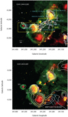 |
Fig. 1. Two-color image of G341.244-00.265: 8 μm emission in green and 24 μm emission in red. The magenta plus signs indicate the eight dense clumps from Contreras et al. (2013). The ATLASGAL 870 μm emissions (in white) are superimposed with levels 0.2, 0.4, 0.8, 1.6, and 3.2 Jy beam−1 in the top panel. The 843 MHz SUMSS radio continuum emissions (in white) are superimposed with levels 0.02, 0.04, 0.08, 0.16, and 0.32 Jy beam−1 in the bottom panel. |
2. Data and analysis
In the following, we present our analysis of archival multiwavelength data from Hi-GAL in Sect. 2.1, ATLASGAL in Sect. 2.2, SEDIGISM in Sect. 2.3, and MALT90 in Sect. 2.4.
2.1. Hi-GAL
The Hi-GAL data set is comprised of five continuum images of the Milky Way Galaxy using the PACS (70 and 160 μm) and SPIRE (250, 350 and 500 μm) instruments. This data set helped us identify an unbiased catalog of filament candidates throughout the Galaxy (e.g., Molinari et al. 2010; André et al. 2010; Wang et al. 2015). The angular resolutions range from 5.2′′ to 35.2′′ for 70 and 500 μm, respectively.The high-frequency bands provide high angular resolution and are less affected by large-scale background and foreground emissions. We made H2 column density and dust temperature maps of this region by the spectral energy distribution (SED) method described by Wang et al. (2015). Given Hi-GAL is sensitive to low-density gas of about 1021 cm−2, background and/or foreground contaminations create a serious problem when analyzing the Hi-GAL data. Following the steps described by Wang et al. (2015), we first removed the background and foreground emissions. After removing the background and foreground emissions, we convolved all images at a resolution of 35′′, which is the beam size of Hi-GAL at 500 μm. For each pixel, we used equation
 (1)
(1)
to model intensities at various wavelengths. The optical depth τν could be estimated through
 (2)
(2)
We adopted a mean molecular weight per H2 molecule of  = 2.8 to include the contributions from helium and other heavy elements. The value mH is the mass of a hydrogen atom,
  is the column density, and R is the gas-to-dust mass ratio, which is set to be 100. According to Ossenkopf & Henning (1994), dust opacity per unit dust mass (κν) could be expressed as
 (3)
(3)
where the value of the dust emissivity index β is fixed to 1.75 in our fitting. The two free parameters ( and Td) for each pixel could be fitted finally. Figure 2 shows the derived H2 column density and dust temperature maps of G341.244-00.265. The morphology of column density is similar to the ATLASGAL 870 μm emissions. The mean H2 column density is 1.9 × 1022 cm−2. The total mass of G341.244-00.265 is ~18919 M⊙ and has a projected length of 11.1 pc. In the head and tail, the gas is much warmer than that in the body of G341.244-00.265. This is probably because the dust there is heated by S22 and S24.
2.2. ATLASGAL clumps
The ATLASGAL also helped us identify an unbiased catalog of filament candidates throughout the Galaxy in the emissions of 870 μm (Li et al. 2016). This is the first systematic survey of the inner Galactic plane in the submillimeter (Siringo et al. 2009; Contreras et al. 2013). It provides high angular resolution (~ 19.2 arcsec) of cold dust emissions in the Galaxy. For a dust temperature of 20 K, ATLASGAL is sensitive to gas with H2 column densities exceeding 1022 cm−2. We found eight dense ATLASGAL clumps from the catalog of Contreras et al. (2013) distributing along this filament like beads on a string. From Table 1, we can see that most of these clumps have masses > 103 M⊙. Given a typical star formation efficiency of 10–30% Lada et al. (2010) [23.5pc] and a cluster having a Salpeter-type initial stellar mass function (IMF), we could expect a 103 M⊙ clump to form a star cluster with massive stars >20 M⊙. Therefore, this filamentary cloud is a candidate of massive star-forming region.
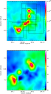 |
Fig. 2. Top panel: H2 column density map of G341.244-00.265 built on the SED fitting pixel by pixel. The seven boxes indicate the seven observed regions by MALT90. Bottom panel: dust temperature Tdust map of G341.244-00.265. The plus signs indicate the dense clumps from Contreras et al. (2013). |
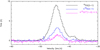 |
Fig. 3. Averaged spectra of 13CO (2–1), C18O (2–1) and H13CO+ (1–0) over the filamentary molecular cloud of G341.244-00.265. |
Physical parameters of the ATLASGAL clumps.
2.3. SEDIGISM
We analyzed 13CO (2–1) and C18O (2–1) emissions in the region of G341.244-00.265 using the Structure, excitation, and dynamics of the inner Galactic interstellar medium (SEDIGISM; Schuller et al. 2017) data. This survey used the lowest frequency module of the Swedish Heterodyne Facility Instrument (SHFI; Vassilev et al. 2008) arrayed on the 12 m Atacama Pathfinder Experiment telescope (APEX), which is located on Llano de Chajnantor in Chile. This project covers a longitude in the range l = − 60° to 18° and a latitude in the range |b| < 0.5° and has a beam size of 28′′. The 4 GHz bandwidth spectrometer consists of two backend units, Fast Fourier Transform Spectrometer-1 (XFFTS-1; Klein et al. 2012)and XFFTS-2. The bandwidth of each unit is 2.5 GHz and has an overlap of 1000 MHz. The velocity resolution is about 0.1 km s−1 at the frequency near 220 GHz. In addition to the CO-isotopolog lines, this survey also includes other transitions such as SO (5–4), SiO (5–4), HC3N (24–23), and so on. According to the APEX telescope efficiencies home page1, the beam efficiency of APEX is 0.75 at the frequency of 230 GHz. A more detail introduction of this survey can be found in Schuller et al. (2017). The 13CO (2–1) and C18O (2–1) cubes are publicly available and can be downloaded from a dedicated server hosted by MPIfR2. Using software packages of CLASS (Continuum and Line Analysis Single-Disk Software) and GREG (Grenoble Graphic), we conducted the data analysis. To compare with the reduced data of Hi-GAL introduced above and the following data of MALT90, a Gaussian smoothing was applied to convolve the SEDIGISM data into a new resolution of 38′′.
Figure 3 shows the averaged spectra of 13CO (2–1) and C18 O (2–1) over the filamentary molecular cloud of G341.244-00.265. It can be seen that two components at velocity intervals −48 to −40 km s−1 and −40 to −36 km s−1 are detected by the two CO isotopologs. The former component is consistent with the ranges measured by Schuller et al. (2017). On the other hand, the −40 to −36 km s−1 component is undetected by H13 CO+ (1–0) in the MALT90 data. Thus, it is likely to be foreground or background emissions unrelated with G341.244-00.265. We made the integrated intensity maps of 13CO (2–1) and C18O (2–1) in the velocity range −48 to −40 km s−1. The emission contours overlaid on the Spitzer-IRAC 8.0 μm, H2 column density, and dust temperature maps derived in Sect. 2.1 are shown in Fig. 4. The regions traced by 13CO (2–1) show an elongated filamentary structure extending from northwest to southeast. On the borders of S22 and S24, a good morphological match can be seen between photodissociation regions (PDRs) and CO emissions, indicating the gas is being compressed by the two infrared bubbles. The C18 O (2–1) emission traces more compact gas than the 13CO (2–1) emission owing to its lower abundance. Most of the C18O emissions come from the head and tail of G341.244-00.265, where the dust temperature is relatively high. In the body, where the dust temperature is around 20 K, the C18 O emission is relatively weak. Chemical models indicate that when Td is below 20 K, carbon species like CO and CS can be depleted in the cold gas (e.g., Lee et al. 2003; Bergin & Tafalla 2007). This may be the reason that the C18O emission is relatively weak in the body of G341.244-00.265.
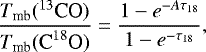
The C18O line is very useful to quantify the column density, as its emissions are optically thin in most cases. We used the C18 O (2–1) to derive the column density by assuming the local thermodynamic equilibrium (LTE) conditions. The optical depth of C18 O (2–1) can be estimated by comparing with its isotopolog line 13CO (2–1). We assumed that the 13CO and C18O emissions arise from the same gas and share a common excitation temperature. The optical depth of the C18 O line could be derived through
 (4)
(4)
where A is their isotope abundance ratio. In this paper, we adopted the isotopic ratio from Wilson & Rood (1994), which depends on the Galactocentric radius of the region,
![Mathematical equation: \begin{equation*}A \equiv \frac{[^{13}\textrm{CO}]}{[{\textrm{C}^{18}\textrm{O}}]} \sim \frac{[^{13}\textrm{C}][^{16}\textrm{O}]}{[^{12}\textrm{C}][^{18}\textrm{O}]} = \frac{58.8 \times R_{\textrm{GC}} [\textrm{kpc}] + 37.1 }{7.5 \times R_{\textrm{GC}} [\textrm{kpc}] + 7.6} ,\end{equation*}](/articles/aa/full_html/2019/02/aa32962-18/aa32962-18-eq8.png) (5)
(5)
where RGC is the distance of the molecular cloud to the Galactic center. By solving Eq. (4) in every map pixel, we obtained the map of τ18, which is shown in the top panel of Fig. 5. The derived τ18 is in the range 0.2 and 0.5, indicating the C18O emission is indeed optically thin in this filamentary cloud.
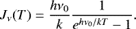
Assuming a filled telescope beam and the excitation temperature is the same for the two isotopic species, we calculated the excitation temperature of C18O using
![Mathematical equation: \begin{equation*}T_{\textrm{ex}} = \frac{h \nu_0}{k} \left[\textrm{ln}\left(1 + \frac{h \nu_0/k}{T_{\textrm{mb}}/(1 - e^{-\tau}) + J_{\nu}(T_{\textrm{bg}})}\right)\right]^{-1} ,\end{equation*}](/articles/aa/full_html/2019/02/aa32962-18/aa32962-18-eq9.png) (6)
(6)
where ν0 is the rest frequency of the transition, Tbg is the temperature of the background radiation (2.73 K), and
 (7)
(7)
Once τ18 and Tex are obtained, the column density of C18O can be calculated through equation
 (8)
(8)
where A is the Einstein coefficient for spontaneous transition, T0 ≡ hν0/k = 10.55 K for C18O (2–1). On the other hand, given C18O (2–1) is optically thin, we used the approximation
 (9)
(9)
The abundance of C18O in each pixel can finally be calculated through χ (C18O) = N(C18O)/N(H2). The column density and abundance maps of C18O are also shown in Fig. 5. The obtained C18 O abundance is (1.9–29.9) × 10−7 and has a mean value of 8.9 × 10⁻⁷. It can be noted that the C18O column density is relatively high on the PDRs around S22 and S24, where the gas is relatively warm. The Td – χ(C18O) relation map in Fig. 6 suggests a positive correlation. This is consistent with chemical model results that as gas gets warmer, more CO species are evaporated from dust grains.
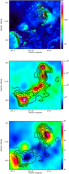 |
Fig. 4. 13CO (black) and C18O (red) line emission contours superimposed on the images of Siptzer-IRAC 8.0 μm (top panel), H2 column density (middle panel), and dust temperature (bottom panel). The emissions are integrated from −48 to −40 km s−1. Contour levels are 40, 50, ..., 90% of each peak emission. |
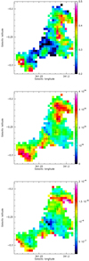 |
Fig. 5. Maps of the optical depth (top panel), column density (middle panel), and abundance (bottom panel) of C18O. The plus signs indicate the dense clumps from Contreras et al. (2013). |
2.4. MALT90
The N2 H+ molecular line data are from MALT90. It is one of the most detected molecules in this survey (e.g., Rathborne 2016). MALT90 is an international project aimed at characterizing the sites within our Galaxy where massive star formation take place (e.g., Foster et al. 2011; Jackson et al. 2013). This project was carried out with the Mopra Spectrometer (MOPS) mounted on the Mopra 22 m telescope, which is located near Coonabarabran in New South Wales, Australia. The full 8 GHz bandwidth of MOPS was split into 16 zoom bands of 138 MHz, providing a velocity resolution of 0.11 km s−1 at frequencies near 90 GHz. The angular resolution of Mopra is 38′′ and has a beam efficiency between 0.49 at 86 GHz and 0.42 at 115 GHz (Ladd et al. 2005). The targets of this survey are selected from the ATLASGAL clumps found by Contreras et al. (2013). The size of the data cube is 4.6′ × 4.6′ and has a step of 9′′. The data files are publicly available and can be downloaded from the MALT90 home page3. We searched theregion of G341.244-00.265 and found seven dust clumps from Contreras et al. (2013) that have been observed by MALT90. The seven regions observed by MALT90 are shown in Fig. 2. We combined the seven data sets into a new data cube by CLASS, keeping the same beam size and spacing between adjacent rows. The new combined image of N2 H+ is shown in Fig. 7.
N2 H+ is a good tracer of dense gas in the early stages of star formation as it is more resistant to freeze-out on grains than the carbon-bearing species (Bergin et al. 2001). The emission maps of N2 H+ overlaid on the Spitzer-IRAC 8 μm, H2 column density, and dust temperature are shown in Fig. 8. We can see that the morphology of N2 H+ integrated intensity is very similar to that of the H2 column density. N2 H+ (1–0) has 15 hyperfine transitions of which 7 have a different frequency (e.g., Pagani et al. 2009; Keto & Rybicki 2010). As shown in Fig. 7, in our filament G341.244-00.265, the 7 hyperfine structures of N2 H+ (1–0) blended into 3 groups because of turbulent line widths. Following the method described by Purcell et al. (2009), we estimate the optical depth of N2 H+ (1–0). Assuming that the line widths of the individual hyperfine components are all equal, the integrated intensities of group 1/group 2 (defined by Purcell et al. 2009) should be in the ratio of 1:5. The optical depth of N2 H+ ( ) can then be derived using the following equation:
 (10)
(10)
By solving Eq. (10) in every map pixel, we obtained the map of  , which is shown in the top panel of Fig. 9. We found that in most part of this molecular cloud, the N2 H+ (1–0) has an intermediate optical depth, ranging from 0.2 to 0.8. Then, we used the following formula to calculate the excitation temperature (Tex) of N2 H+:
 (11)
(11)
Assuming LTE conditions and a beam filling factor of 1, the column density of N2 H+ in every pixel can thus be calculated through
 (12)
(12)
where c is the velocity of light in the vacuum, ν is the frequency of the transition, gu is the statistical weight of the upper level, Aul is the Einstein coefficient, El is the energy of the lower level, and Qrot is the partition function. We used the approximation
 (13)
(13)
to take  into account. The abundance of N2 H+ in each pixel can be calculated through χ (N2 H+) = N(N2H+)/N(H2). The column density and abundance maps of N2 H+ is also shown in Fig. 9. In G341.244-00.265, the column density of N2 H+ ranges from 2.1 × 10¹² to 1.8 × 1013 cm−2 and has a mean value of 0.9 × 1013 cm−2. In the dense part of this molecular cloud, the morphology of N2 H+ column density is very similar to that of
  , suggesting N2 H+ is really a good tracer for dense gas.
Chemical models indicate that in the early stages of star formation, as the cloud collapses and the density increases, C-species including CO are easy to be absorbed onto the dust surface, while N-bearing species such as NH3 and N2 H+ are hardly depleted. As the central star evolves, the molecular cloud gets warm and CO is evaporated from the dust grains when the dust temperature exceeds ~20 K (Tobin et al. 2013). N2 H+ could be destroyed by CO through N2 H+ + CO → HCO+ + N2 (e.g., Bergin & Langer 1997; Lee et al. 2004; Yu & Xu 2016). When HII regions have formed, N2 H+ could also be destroyed by the electron recombination N2 H+ + e− → N2 + H or NH + N (e.g., Busquet et al. 2011; Dislaire et al. 2012; Vigren et al. 2012; Yu & Xu 2016). Thus, the N(N2H+)/N(C18O) ratio could be used as a chemical clock for cloud evolution in star-forming regions. We would expect to find that this ratio decreases as the molecular cloud evolves. Figure 10 shows the map of N(N2H+)/N(C18O) relative abundance ratio. We can see that in the center of G341.244-00.265, the ratio is relatively high compared to the other parts of this filament. We regard the gas in the center of G341.244-00.265 as less evolved.
 |
Fig. 6. Abundance of C18O plotted as a function of dust temperature in each pixel of G341.244-00.265. |
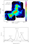 |
Fig. 7. Top panel: new combined image of N2H+ from MALT90 data set. The emission has been integrated from −46 to −40 km s−1. Bottom panel: averaged spectra of N2H+ over the cloud of G341.244-00.265. The vertical dashed lines indicate the seven hyperfine structures. |
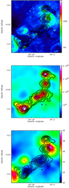 |
Fig. 8. N2H+ emission contours superimposed on the images of Spitzer-IRAC 8.0 μm (top panel), H2 column density (middle panel), and dust temperature (bottom panel). Contour levels are from 2.5 to 8.5 in step of 1.0 K km s−1. |
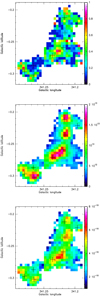 |
Fig. 9. Maps of the optical depth (top panel), column density (middle panel), and abundance (bottom panel) of N2H+ (1–0). The plus signs indicate the dense clumps from Contreras et al. (2013). |
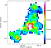 |
Fig. 10. N(N2H+)/N(C18O) relative abundance ratio map of G341.244-00.265. The plus signs indicate the dense clumps from Contreras et al. (2013). |
2.5. Ionizing luminosity and ages of S22 and S24
We used the SUMSS 834 MHz radio continuum data to estimate the Lyman continuum fluxes and dynamical ages of S22 and S24. Assuming an electron temperature of Te = 104 K, the number of UV ionizing photons needed to keep an HII region ionized is given by (Chaisson 1976; Guzmán et al. 2012)
 (14)
(14)
where ν is the frequency and Sν is the integrated flux density, and D is the kinematic distance (3.6 kpc) to the HII region. We derived NL ~ 9.3 × 1047 ph s−1 and 9.0 × 1047 ph s−1 for S22 and S24, respectively. Based on the ionizing fluxes for massive stars given by Martins et al. (2005), we estimated the spectral types of the ionizing stars of S22 and S24 to be O9.5V.
Assuming the two HII regions expand in a homogeneous medium, their dynamical ages could be estimated through (Dyson & Williams 1980)
![Mathematical equation: \begin{equation*}t_{\textrm{dyn}} = \frac{4 R_{\textrm{s}}}{7 c_{\textrm{s}}} \left[\left(\frac{R_{\textrm{HII}}}{R_{\textrm{s}}}\right)^{7/4} - 1\right] ,\end{equation*}](/articles/aa/full_html/2019/02/aa32962-18/aa32962-18-eq22.png) (15)
(15)
where cs is the sound velocity in the ionized gas, assumed to be 10 km s−1; RHII is the radius of the HII region; Rs is the original Strömgren radius given by Rs = (3NL/4 )1∕3, where NL is the ionizing luminosity calculated above; ni is the initial H number density of the gas; and αB = 2.6 × 10⁻¹³ cm3 s−1 is the hydrogen recombination coefficient. We found the dynamical ages are about 2.1 × 10⁵ and 2.2 × 10⁵ yr for S22 and S24, respectively.
2.6. Distributions of YSOs
We used the highly reliable GLIMPSE I catalog to search for YSOs in this filamentary cloud. The regions in the top panel of Fig. 11 indicate stellar evolutionary stages based on the criteria described by Allen et al. (2004): Class II sources are disk-dominated objects. These objects lie in the region 0 < [3.6]-[4.5] < 0.8 and 0.4 < [5.8]-[8.0] < 1.1, and their IR excess is caused by accretion disks around the YSOs. Class I sources are protostars with interstellar envelopes. Their locations in the color-color [3.6]-[4.5] vs. [5.8]-[8.0] diagram are delineated by the green lines in Fig. 11. We also used photometric data from the WISE survey to identify YSO candidates in this region. According to the criteria of Koenig et al. (2012), Class I candidates are selected if their colors match [3.4]-[4.6] > 1.0 and [4.6]-[12.0] > 2.0, while ClassII candidates are selected with colors [3.4]-[4.6] > 0.25 + σ ([3.4]-[4.6]) and [4.6]-[12.0] > 1.0 + σ ([4.6]-[12.0]), where σ(...) indicates a combined error, added in quadrature. The locations of Class I and Class II candidates in color–color diagrams (CCDs) are shown in Fig. 11. The spatial distributions of the selected YSOs are shown in Fig. 12. We note that most ofthe YSOs distributed in the center of this filament are Class I sources, while most Class II candidates are located in the head and tail of G341.244-00.265, indicating star formation activities began on the two ends of this filament first.
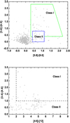 |
Fig. 11. Top panel: GLIMPSE [5.8]-[8.0] vs. [3.6]-[4.5] diagram for selected sources in the region of G345.244-00.265. Class I and Class II regions are indicated according to the criteria given by Allen et al. (2004). Bottom panel: YSO candidates from the WISE database. |
3. Discussions
3.1. Fragmentation
The gravitational stability of a filament can be estimated by comparing its linear mass density (M∕l) with the virial linear mass density ((M∕l)vir ≡ 2 /G). The value σv is the one-dimensional total (thermal plus nonthermal) velocity dispersion of the average molecular gas. We derived the velocity dispersion from the average FWHM of C18 O (2–1) line. The linear mass per unit length (M∕l) of G341.244-00.265 is about 1654 M⊙ pc−1, while the virial linear mass density is only about 627 M⊙ pc−1, indicating turbulence inside is unable to prevent the cloud from gravitational collapse. From the ATLASGAL catalog of Contreras et al. (2013), we found eight dense clumps involved in this region. Half of these (AGAL341.217-00.212, AGAL341.219-00.259, AGAL341.236-00.271, and AGAL341.266-00.302) show infall motions (He et al. 2015), indicating star formation activities are ongoing actively in this filamentary cloud. We consider the mass-size relationship of these clumps to find out whether they have sufficient mass to form massive stars. The effective radius can be determined by r =
  . In this case, Lmaj and Lmin are the deconvolved major and minor axes of each clump. According to Kauffmann & Pillai (2010), the threshold for massive star formation is M(r) ≥ 870 M⊙ (r∕pc)1.33. Figure 13 presents the mass versus radius plot of the eight clumps embedded in G341.244-00.265. We found all these dense clumps lie above the threshold, indicating they are candidates of massive star formation regions.
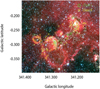 |
Fig. 12. Spacial distributions of YSOs on the three-color image created using the Spitzer 3.6 (blue), 4.5 (green), and 8.0 (red) μm IRAC band filters. Class I candidates are shown by green circles, while Class II candidates are shown by yellow crosses. The white contours are the same as shown in the top panel of Fig. 1. |
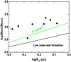 |
Fig. 13. Mass vs. radius plot of the eight clumps embedded in G341.244-00.265. The region below the black line represents the space devoid of massive star formation, where M(r) < 870 M⊙(r∕pc)1.33 (Kauffmann & Pillai 2010). |
3.2. Dynamic structure of the filament
The dynamic structure can be a useful tool to study the formation and evolution of a filament. Velocity gradients perpendicular to the major axis have been postulated as effects of filament rotation (Olmi & Testi 2002) and/or convergent flows (Schneider et al. 2010). On the other hand, velocity gradients along filaments have been explained as mass inflowing toward the cloud cores (e.g., Kirk et al. 2013; Dhabal et al. 2018). Figure 14 presents the complex velocity-field (moment 1) map of G341.244-00.265 from the 13CO; the N2 H+ moment 1 map is not shown as they look very similar. At least two projected velocity gradients have been observed. The direction of velocity gradient 1 is toward S22 and has a value of about 0.85 km s−1 pc−1. The CO molecular gas shows an arc-like structure around S22. The turbulent energy of the PDR around S22 could be estimated through Eturb =  , where σ3d ≈
  σv, which is the three-dimensional turbulent velocity dispersion. The derived turbulent energy of the PDR around S22 is about 1.2 × 1047 erg. The ionization energy and thermal energy of S22 can be estimated as (Freyer et al. 2003)
 (16)
(16)
 (17)
(17)
where χ0 is the ionization potential (13.6 eV) of hydrogen in the ground state. We found the ionization energy and thermal energy of S22 are about 5.1 × 1047 erg and 0.3 × 1047 erg, respectively. The ionization energy of S22 is 4 times larger than its surrounding PDR turbulent energy. Thus, we regard S22 as the likely driving source of velocity gradient 1. The direction of velocity gradient 2 is from southwest to northeast and has a value of 0.62 km s−1 pc−1. In Fig. 1, we can see that there seems to be an ionized shock in the southwest of G341.244-00.265. Bubble MWP1G341176-003905 may be the driving source for velocity gradient 2. However, the SUMSS radio emission of MWP1G341176-003905 is very irregular. We could not estimate its ionization energy and thermal energy. If S22 and MWP1G341176-003905 are indeed the driving sources of the two velocity gradients, our study indicates that at least part of the large-scale dynamics in G341.244-00.265 originate from turbulence injections. The velocity gradients in the head are very complex. They cannot be explained by a single ration of the filament and/or shocks from bubble S24.
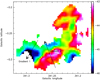 |
Fig. 14. Velocity-field (moment 1) map of 13CO (2–1) of G341.244-00.265. |
3.3. Star formation scenario
The distributions of YSOs suggest there is an age gradient of star formation in this filamentary cloud: most of the YSOs distributed in the center of this filament are Class I sources, while most Class II candidates are located in the head and tail of G341.244-00.265, indicating star formation activities began on the two ends of this filament first. The abundance ratio of N(N2H+)/N(C18O) is relatively higher in the center than that in the two ends of G341.244-00.265, also indicating the gas in the center is less evolved. Both observations and theories indicate expanding HII regions may trigger the next generation of star formation (e.g., Cichowolski et al. 2009; Miao et al. 2009; Panwar et al. 2014). Triggered star formation scenario indicates there should be an age gradient: the ages of stars decrease from the center to the outside of an expanding HII region. According to André & Montmerle (1994), the age of Class I YSOs is ~105 yr, while ClassII YSOs have a timescale of ~106 yr. However, the dynamical age of S22 and S24 is only about 2.2 × 10⁵ yr. They are too young to trigger the star formation of the surrounding Class II YSOs. The study of Cappa et al. (2016) also indicates that bubble S24 is too young for triggering to have begun. Thus the age gradient could not be explained by the triggered star formation scenario. Numerical studies show that in a long but finite-sized filament, collapse may act a factor of two to three times faster at the ends of the filament than at its center (e.g., Pon et al. 2011, 2012), suggesting star formation at the ends of the filament prior to its center. Recently, Kainulainen et al. (2016) found the fragmentation strongly at the ends of the Musca cloud. Dewangan et al. (2017) also found massive clumps and YSO clusters prefer to locate at the both ends of the filamentary molecular cloud S242. These authors suggest the so-called end-dominated collapse may be responsible. Taking into account the distributions of YSOs and the N(N2H+)/N(C18O) ratio map, our study is also in agreement with the prediction of the so-called end-dominated collapse star formation scenario.
4. Summary
We performed a multiwavelength study toward molecular cloud G341.244-00.265 to investigate the physical and chemical properties, as well as the star formation activities taking place therein. The cloud shows an elongated filamentary structure both in far-infrared and molecular line emissions, with its head and tail associated with infrared bubbles S21, S22, and S24. G341.244-00.265 has a linear mass density of about 1654 M⊙ pc−1 and has a projected length of 11.1 pc. The cloud is prone to collapse based on the virial analysis. From the ATLASGAL catalog, we found eight dense massive clumps associated with this filamentary cloud. All of these clumps have sufficient mass to form massive stars. At least two velocity gradients have been found. S22 and MWP1G341176-003905 may be the driving source of the two velocity gradients. Using data from the GLIMPSE and WISE survey, we searched for YSO candidates in this region. We found an age gradient of star formation in this filamentary cloud: most of the YSOs distributed in the center are Class I sources, while most Class II candidates are located on the two ends of G341.244-00.265, indicating star formation at the two ends of this filament is prior to the center. The abundance ratio of N(N2H+)/N(C18O) is higher in the center than that in the two ends, also indicating the gas in the center is less evolved. Taking into account the distributions of YSOs and the N(N2H+)/N(C18O) ratio map, our study is in agreement with the prediction of the so-called end-dominated collapse star formation scenario.
Acknowledgements
We are very grateful to the anonymous referee for his/her helpful comments and suggestions. This paper has made use of information from the APEX Telescope Large Area Survey of the Galaxy. The ATLASGAL project is a collaboration between the Max-Planck-Gesellschaft, the European Southern Observatory (ESO) and the Universidad de Chile. This research made use of data products from the Millimeter Astronomy Legacy Team 90 GHz (MALT90) survey. The Mopra telescope is part of the Australia Telescope and is funded by the Commonwealth of Australia for operation as National Facility managed by CSIRO. This paper is supported by National Natural Science Foundation of China under grants of 11503037.
References
- Allen, L. E., Calvet, N., D’Alessio, P., et al. 2004, ApJS, 154, 363 [NASA ADS] [CrossRef] [Google Scholar]
- André, P., & Montmerle, T. 1994, ApJ, 420, 837 [NASA ADS] [CrossRef] [Google Scholar]
- André, P., Men’shchikov, A., Bontemps, S., et al. 2010, A&A, 518, L102 [NASA ADS] [CrossRef] [EDP Sciences] [Google Scholar]
- Battisti, A. J.,& Heyer, M. H. 2014, ApJ, 780, 173 [NASA ADS] [CrossRef] [EDP Sciences] [Google Scholar]
- Bergin, E. A., & Langer, W. D. 1997, ApJ, 486, 316 [NASA ADS] [CrossRef] [Google Scholar]
- Bergin, E. A., & Tafalla, M. 2007, ARA&A, 45, 339 [NASA ADS] [CrossRef] [Google Scholar]
- Bergin, E. A., Ciardi, D. R., Lada, C. J., Alves, J., & Lada, E. A. 2001, ApJ, 557, 209 [NASA ADS] [CrossRef] [Google Scholar]
- Busquet, G., Estalella, R., Zhang, Q., et al. 2011, A&A, 525, A141 [NASA ADS] [CrossRef] [EDP Sciences] [Google Scholar]
- Cappa, C. E., Duronea, N., Firpo, V., et al. 2016, A&A, 585, 30 [Google Scholar]
- Chaisson, E. J. 1976, in Frontiers of Astrophysics, ed. E. H. Avrett (Harvard: Harvard University Press), 259 [Google Scholar]
- Chen, X., Shen, Z., Li, J., Xu, Y., & He, J. 2010, ApJ, 710, 150 [NASA ADS] [CrossRef] [Google Scholar]
- Cichowolski, S., Romero, G. A., Ortega, M. E., Cappa, C. E., & Vasquez, J. 2009, MNRAS, 394, 900 [NASA ADS] [CrossRef] [Google Scholar]
- Contreras, Y., Schuller, F., Urquhart, J. S., et al. 2013, A&A, 549, A45 [NASA ADS] [CrossRef] [EDP Sciences] [Google Scholar]
- Contreras, Y., Rathborne, J. M., Guzman, A., et al. 2017, MNRAS, 466, 340 [NASA ADS] [CrossRef] [Google Scholar]
- Cyganowski, C. J., Whitney, B. A., Holden, E., et al. 2008, AJ, 136, 2391 [NASA ADS] [CrossRef] [Google Scholar]
- Cyganowski, C. J., Brogan, C. L., Hunter, T. R., Churchwell, E., & Zhang, Q. 2011, ApJ, 729, 124 [NASA ADS] [CrossRef] [Google Scholar]
- Deharveng, L., Schuller, F., Anderson, L. D., et al. 2010, A&A, 523, A6 [NASA ADS] [CrossRef] [EDP Sciences] [Google Scholar]
- Dewangan, L. K., Baug, T., Ojha, D. K., et al. 2017, ApJ, 845, 34 [NASA ADS] [CrossRef] [Google Scholar]
- Dhabal, A., Mundy, L. G., Rizzo, M. J., Storm, S., & Teuben, P. 2018, ApJ, 853, 169 [NASA ADS] [CrossRef] [Google Scholar]
- Dislaire, V., Hily-Blant, P., Faure, A., et al. 2012, A&A, 537, A20 [NASA ADS] [CrossRef] [EDP Sciences] [Google Scholar]
- Dyson, J. E., & Williams, D. A. 1980, Physics of the Interstellar Medium (Manchester: Manchester University Press) [Google Scholar]
- Enoch, M. L., Young, K. E., Glenn, J., et al. 2006, ApJ, 638, 293 [NASA ADS] [CrossRef] [Google Scholar]
- Freyer, T., Hensler, G., & Yorke, H. W. 2003, ApJ, 594, 888 [NASA ADS] [CrossRef] [Google Scholar]
- Foster, J. B., Jackson, J. M., Barnes, P. J., et al. 2011, ApJS, 197, 25 [NASA ADS] [CrossRef] [Google Scholar]
- Fuente, A., Martin-Pintado, J., Cernicharo, J., & Bachiller, R. 1993, A&A, 276, 473 [NASA ADS] [Google Scholar]
- Guzmán, A., Garay, G., Brooks, K. J., & Voronkov, M. A. 2012, ApJ, 753, 51 [NASA ADS] [CrossRef] [Google Scholar]
- Guzmán, A., Sanhueza, P., Contreras, Y., et al. 2015, ApJ, 815, 130 [NASA ADS] [CrossRef] [Google Scholar]
- He, Y. X., Zhou, J. J., Esimbek, J., et al. 2015, MNRAS, 450, 1926 [NASA ADS] [CrossRef] [Google Scholar]
- Jackson, J. M., Rathborne, J. M., Foster, J. B., et al. 2013, PASA, 30, 57 [CrossRef] [Google Scholar]
- Kainulainen, J., Hacar, A., Alves, J., et al. 2016, A&A, 586, A27 [NASA ADS] [CrossRef] [EDP Sciences] [Google Scholar]
- Kauffmann, J., & Pillai, T. 2010, ApJ, 723, L7 [NASA ADS] [CrossRef] [Google Scholar]
- Keto, E., & Rybicki, G. 2010, ApJ, 716, 1315 [NASA ADS] [CrossRef] [Google Scholar]
- Kirk, H., Myers, P. C., Bourke, T. L., et al. 2013, ApJ, 766, 115 [NASA ADS] [CrossRef] [Google Scholar]
- Klein, B., Hochgürtel, S., Krämer, I., et al. 2012, A&A, 542, L3 [NASA ADS] [CrossRef] [EDP Sciences] [Google Scholar]
- Koenig, X. P., Leisawitz, D. T., Benford, D. J., et al. 2012, ApJ, 744, 130 [NASA ADS] [CrossRef] [Google Scholar]
- Lada, C. J., Lombardi, M., & Alves, J. F. 2010, ApJ, 724, 687 [NASA ADS] [CrossRef] [Google Scholar]
- Ladd, N., Purcell, C., Wong, T., & Robertson, S. 2005, PASA, 22, 62 [NASA ADS] [CrossRef] [Google Scholar]
- Lee, J. E., Evans, N. J., II, Shirley, Y. L., & Tatematsu, K. 2003, ApJ, 583, 789 [NASA ADS] [CrossRef] [Google Scholar]
- Lee, J. E., Bergin, E. A., & Evans, N. J. 2004, ApJ, 617, 360 [NASA ADS] [CrossRef] [Google Scholar]
- Li, G.-X., Urquhart, J. S., Leurini, S., et al. 2016, A&A, 591, A5 [NASA ADS] [CrossRef] [EDP Sciences] [Google Scholar]
- Martins, F., Schaerer, D., & Hillier, D. J. 2005, A&A, 436, 1049 [NASA ADS] [CrossRef] [EDP Sciences] [Google Scholar]
- Mauch, T., Murphy, T., Buttery, H. J., et al. 2003, MNRAS, 342, 1117 [NASA ADS] [CrossRef] [Google Scholar]
- Miao, J., White, G. J., Thompson, M., & Nelson, R. 2009, ApJ, 692, 382 [NASA ADS] [CrossRef] [Google Scholar]
- Molinari, S., Swinyard, B., Bally, J., et al. 2010, A&A, 518, L100 [NASA ADS] [CrossRef] [EDP Sciences] [Google Scholar]
- Moore, T. J. T., Bretherton, D. E., Fujiyoshi, T., et al. 2007, MNRAS, 379, 663 [NASA ADS] [CrossRef] [Google Scholar]
- Olmi, L., & Testi, L. 2002, A&A, 392, 1053 [NASA ADS] [CrossRef] [EDP Sciences] [Google Scholar]
- Ossenkopf, V., & Henning T. 1994, A&A, 291, 943 [NASA ADS] [Google Scholar]
- Pagani, L., Daniel, F., & Dubernet, M.-L. 2009, A&A, 494, 719 [NASA ADS] [CrossRef] [EDP Sciences] [Google Scholar]
- Panwar, N., Chen, W. P., Pandey, A. K., et al. 2014, MNRAS, 443, 1614 [NASA ADS] [CrossRef] [Google Scholar]
- Pon, A., Johnstone, D., & Heitsch, F. 2011, ApJ, 740, 88 [NASA ADS] [CrossRef] [Google Scholar]
- Pon, A., Toalá, J. A., Johnstone, D., et al. 2012, ApJ, 756, 145 [NASA ADS] [CrossRef] [Google Scholar]
- Purcell, C. R., Longmore, S. N., Burton, M. G., et al. 2009, MNRAS, 394, 323 [NASA ADS] [CrossRef] [Google Scholar]
- Ragan, S. E., Henning, T., Tackenberg, J., et al. 2014, A&A, 568, A73 [NASA ADS] [CrossRef] [EDP Sciences] [Google Scholar]
- Rathborne, J. M., Whitaker, J. S., Jackson, J. M., et al. 2016, PASA, 33, e030 [NASA ADS] [CrossRef] [Google Scholar]
- Schneider, N., Csengeri, T., Bontemps, S., et al. 2010, A&A, 520, A49 [NASA ADS] [CrossRef] [EDP Sciences] [Google Scholar]
- Schuller, F., Menten, K. M., Contreras, Y., et al. 2009, A&A, 504, 415 [NASA ADS] [CrossRef] [EDP Sciences] [Google Scholar]
- Schuller, F., Csengeri, T., Urquhart, J. S., et al. 2017, A&A, 601, A124 [NASA ADS] [CrossRef] [EDP Sciences] [Google Scholar]
- Simpson, R. J., Povich, M. S., Kendrew, S., et al. 2012, MNRAS, 424, 2442 [NASA ADS] [CrossRef] [Google Scholar]
- Siringo, G., Kreysa, E., Kovács, A., et al. 2009, A&A, 497, 945 [NASA ADS] [CrossRef] [EDP Sciences] [Google Scholar]
- Tobin, J. J., Bergin, E. A., Hartmann, L., et al. 2013, ApJ, 765, 18 [NASA ADS] [CrossRef] [Google Scholar]
- Vassilev, V., Meledin, D., Lapkin, I., et al. 2008, A&A, 490, 1157 [NASA ADS] [CrossRef] [EDP Sciences] [Google Scholar]
- Vigren, E., Zhaunerchyk, V., Hamberg, M. et al. 2012, ApJ, 757, 34 [NASA ADS] [CrossRef] [Google Scholar]
- Wang, K., Testi, L., Ginsburg, A., et al. 2015, MNRAS, 450, 4043 [NASA ADS] [CrossRef] [MathSciNet] [Google Scholar]
- Whitworth, A. P., Bhattal, A. S., Chapman, S. J., Disney, M. J., & Turner, J. A. 1994, MNRAS, 268, 291 [NASA ADS] [CrossRef] [Google Scholar]
- Wilson, T. L., & Rood, R. 1994, ARA&A, 32, 191 [NASA ADS] [CrossRef] [Google Scholar]
- Yu, N. P., & Xu J. L. 2016, ApJ, 833, 248 [NASA ADS] [CrossRef] [Google Scholar]
- Zinnecher, H., & Yorke, H. W. 2007, ARA&A, 45, 481 [NASA ADS] [CrossRef] [Google Scholar]
All Tables
All Figures
|
Fig. 1. Two-color image of G341.244-00.265: 8 μm emission in green and 24 μm emission in red. The magenta plus signs indicate the eight dense clumps from Contreras et al. (2013). The ATLASGAL 870 μm emissions (in white) are superimposed with levels 0.2, 0.4, 0.8, 1.6, and 3.2 Jy beam−1 in the top panel. The 843 MHz SUMSS radio continuum emissions (in white) are superimposed with levels 0.02, 0.04, 0.08, 0.16, and 0.32 Jy beam−1 in the bottom panel. |
| In the text | |
|
Fig. 2. Top panel: H2 column density map of G341.244-00.265 built on the SED fitting pixel by pixel. The seven boxes indicate the seven observed regions by MALT90. Bottom panel: dust temperature Tdust map of G341.244-00.265. The plus signs indicate the dense clumps from Contreras et al. (2013). |
| In the text | |
|
Fig. 3. Averaged spectra of 13CO (2–1), C18O (2–1) and H13CO+ (1–0) over the filamentary molecular cloud of G341.244-00.265. |
| In the text | |
|
Fig. 4. 13CO (black) and C18O (red) line emission contours superimposed on the images of Siptzer-IRAC 8.0 μm (top panel), H2 column density (middle panel), and dust temperature (bottom panel). The emissions are integrated from −48 to −40 km s−1. Contour levels are 40, 50, ..., 90% of each peak emission. |
| In the text | |
|
Fig. 5. Maps of the optical depth (top panel), column density (middle panel), and abundance (bottom panel) of C18O. The plus signs indicate the dense clumps from Contreras et al. (2013). |
| In the text | |
|
Fig. 6. Abundance of C18O plotted as a function of dust temperature in each pixel of G341.244-00.265. |
| In the text | |
|
Fig. 7. Top panel: new combined image of N2H+ from MALT90 data set. The emission has been integrated from −46 to −40 km s−1. Bottom panel: averaged spectra of N2H+ over the cloud of G341.244-00.265. The vertical dashed lines indicate the seven hyperfine structures. |
| In the text | |
|
Fig. 8. N2H+ emission contours superimposed on the images of Spitzer-IRAC 8.0 μm (top panel), H2 column density (middle panel), and dust temperature (bottom panel). Contour levels are from 2.5 to 8.5 in step of 1.0 K km s−1. |
| In the text | |
|
Fig. 9. Maps of the optical depth (top panel), column density (middle panel), and abundance (bottom panel) of N2H+ (1–0). The plus signs indicate the dense clumps from Contreras et al. (2013). |
| In the text | |
|
Fig. 10. N(N2H+)/N(C18O) relative abundance ratio map of G341.244-00.265. The plus signs indicate the dense clumps from Contreras et al. (2013). |
| In the text | |
|
Fig. 11. Top panel: GLIMPSE [5.8]-[8.0] vs. [3.6]-[4.5] diagram for selected sources in the region of G345.244-00.265. Class I and Class II regions are indicated according to the criteria given by Allen et al. (2004). Bottom panel: YSO candidates from the WISE database. |
| In the text | |
|
Fig. 12. Spacial distributions of YSOs on the three-color image created using the Spitzer 3.6 (blue), 4.5 (green), and 8.0 (red) μm IRAC band filters. Class I candidates are shown by green circles, while Class II candidates are shown by yellow crosses. The white contours are the same as shown in the top panel of Fig. 1. |
| In the text | |
|
Fig. 13. Mass vs. radius plot of the eight clumps embedded in G341.244-00.265. The region below the black line represents the space devoid of massive star formation, where M(r) < 870 M⊙(r∕pc)1.33 (Kauffmann & Pillai 2010). |
| In the text | |
|
Fig. 14. Velocity-field (moment 1) map of 13CO (2–1) of G341.244-00.265. |
| In the text | |
Current usage metrics show cumulative count of Article Views (full-text article views including HTML views, PDF and ePub downloads, according to the available data) and Abstracts Views on Vision4Press platform.
Data correspond to usage on the plateform after 2015. The current usage metrics is available 48-96 hours after online publication and is updated daily on week days.
Initial download of the metrics may take a while.