| Issue |
A&A
Volume 622, February 2019
|
|
|---|---|---|
| Article Number | A67 | |
| Number of page(s) | 18 | |
| Section | Stellar structure and evolution | |
| DOI | https://doi.org/10.1051/0004-6361/201731913 | |
| Published online | 30 January 2019 | |
Magnetic characterization and variability study of the magnetic SPB star o Lupi
1
LESIA, Observatoire de Paris, PSL Research University, CNRS, Sorbonne Universités, UPMC Univ. Paris 06, Univ. Paris Diderot, Sorbonne Paris Cité, 5 place Jules Janssen, 92195 Meudon, France
e-mail: This email address is being protected from spambots. You need JavaScript enabled to view it.
2
Instituut voor Sterrenkunde, KU Leuven, Celestijnenlaan 200D, 3001 Leuven, Belgium
3
Department of Physics, California Lutheran University, 60 West Olsen Road # 3700, Thousand Oaks, CA 91360, USA
4
Dept. of Astrophysics, IMAPP, Radboud University Nijmegen, 6500 GL Nijmegen, The Netherlands
5
Université Grenoble Alpes, CNRS, IPAG, 38000 Grenoble, France
Received:
7
September
2017
Accepted:
7
August
2018
Abstract
Thanks to large dedicated surveys, large-scale magnetic fields have been detected for about 10% of early-type stars. We aim to precisely characterize the large-scale magnetic field of the magnetic component of the wide binary o Lupi, by using high-resolution ESPaDOnS and HARPSpol spectropolarimetry to analyze the variability of the measured longitudinal magnetic field. In addition, we have investigated the periodic variability using space-based photometry collected with the BRITE-Constellation by means of iterative prewhitening. The rotational variability of the longitudinal magnetic field indicates a rotation period Prot = 2.95333(2) d and that the large-scale magnetic field is dipolar, but with a significant quadrupolar contribution. Strong differences in the strength of the measured magnetic field occur for various chemical elements as well as rotational modulation for Fe and Si absorption lines, suggesting a inhomogeneous surface distribution of chemical elements. Estimates of the geometry of the large-scale magnetic field indicate i = 27 ± 10°, β = 74−9+7°, and a polar field strength of at least 5.25 kG. The BRITE photometry reveals the rotation frequency and several of its harmonics, as well as two gravity mode pulsation frequencies. The high-amplitude g-mode pulsation at f = 1.1057 d−1 dominates the line-profile variability of the majority of the spectroscopic absorption lines. We do not find direct observational evidence of the secondary in the spectroscopy. Therefore, we attribute the pulsations and the large-scale magnetic field to the B5IV primary of the o Lupi system, but we discuss the implications should the secondary contribute to or cause the observed variability.
Key words: stars: magnetic field / stars: rotation / stars: oscillations / stars: early-type / stars: individual: o Lupi
© ESO 2019
1. Introduction
Large-scale magnetic fields are detected at the stellar surface of about 10% of the studied early-type stars by measuring their Zeeman signature in high-resolution spectropolarimetry (e.g., MiMeS, Wade et al. 2016; the BOB campaign, Morel et al. 2015; and the BRITE spectropolarimetric survey, Neiner et al. 2017). These large-scale magnetic fields appear to be stable over a timescale of decades, have a rather simple geometry (most often a magnetic dipole), and have a polar strength ranging from about 100 G to several tens of kG. Because the fields remain stable and their properties do not depend on any observed stellar parameters, we expect that these large-scale magnetic fields were produced during earlier stages of the star’s life, relaxing into the observed configuration (e.g., Mestel 1999; Neiner et al. 2015). In addition, a dynamo magnetic field is likely to occur in the deep interior of early-type stars, produced by the convective motions of ionized matter in the convective core (Moss 1989). However, no direct evidence of such a magnetic dynamo has ever been observed at the stellar surface, nor is it expected, since the Ohmic diffusion timescale from the core to the surface is longer than the stellar lifetime.
The large-scale magnetic fields detected at the surface of early-type stars have implications on the properties of the circumstellar environment, the stellar surface, and the interior, altering the star’s evolution. The ionized wind material follows the magnetic field lines, and can create (quasi-)stable structures in the circumstellar environment or magnetosphere. The precise properties of the magnetospheric material depend on the stellar and magnetic properties (e.g., ud-Doula & Owocki 2002; Townsend & Owocki 2005). In general, magnetospheres are subdivided into centrifugal magnetospheres, where material remains trapped by the magnetic field and supported against gravity by rapid rotation, and dynamical magnetospheres. The latter has a region of enhanced density in the circumstellar environment that continuously accumulates new wind material and loses matter to accretion by the star.
At the stellar surface, the large-scale magnetic field can affect the stratification and diffusion of certain chemical species at the surface, which can cause surface abundance inhomogeneities of certain chemical elements, and a peculiar global photospheric abundance composition. This would lead to rotational modulation of line profiles and photometric variability. Stars for which such peculiarities are observed are denoted by the Ap/ Bp spectral classification.
The structure and evolution of the deep stellar interior is anticipated to be altered by the large-scale magnetic field, due to the competition of the Lorentz force with the pressure force and gravity. This leads to a uniformly rotating radiative envelope (e.g., Ferraro 1937; Moss 1992; Spruit 1999; Mathis & Zahn 2005; Zahn et al. 2011), altering the depth over which material overshoots the convective core boundary into the radiative layer (e.g., Press 1981; Browning et al. 2004). Currently, this effect has only been determined for two stars with a technique referred to as magneto-asteroseismology, which combines the analysis of the star’s pulsations with that of its magnetic properties, and then performing forward seismic modeling. This was done for the magnetic β Cep pulsator V 2052 Oph (Neiner et al. 2012; Handler et al. 2012; Briquet et al. 2012) and the magnetic g-mode pulsator HD 43317 (Buysschaert et al. 2017a, 2018).
Whenever present, the properties of the stellar pulsations depend on the strength, geometry and orientation of the large-scale magnetic field (e.g., Biront et al. 1982; Gough & Taylor 1984; Dziembowski & Goode 1985, 1996; Gough & Thompson 1990; Goode & Thompson 1992; Shibahashi & Takata 1993; Takata & Shibahashi 1995; Bigot et al. 2000; Hasan et al. 2005; Mathis & de Brye 2011; Lecoanet et al. 2017). For stars with a spectral type from O9 to B2, β Cep-type pulsations are expected. These are low-order pressure modes with periods on the order of several hours. For slightly less massive stars (spectral types B2 to B9) Slowly Pulsating B-type (SPB) oscillations are predicted. These are low-degree, high-order gravity modes with a period on the order of a few days. Moreover, their pulsation modes show a regular pattern in the period domain. Both the β Cep and SPB pulsations are driven by the κ-mechanism, related to the temperature dependent opacity of iron-like elements. In addition gravito-intertial modes, which are excited by the motions of the convective core and have the Coriolis force and buoyancy as restoring forces, are anticipated for early-type stars with periods longer than the stellar rotation period (e.g., Mathis et al. 2014). Stellar pulsations remain the sole way to probe the interior of a single star, with the parameters of the pulsation modes dependent on the conditions inside the star.
Variability due to gravity waves (e.g., Press 1981; Rogers et al. 2013) was recently also found in photospheric and wind lines of the O9Iab star HD 188209 (Aerts et al. 2017), the B1Ia star HD 2905 (Simón-Díaz et al. 2018), and the B1Iab star ρ Leo (Aerts et al. 2018), as well as in the close binary V380 Cyg (Tkachenko et al. 2014). The presence of gravity waves seems to be a common property of hot massive stars that have evolved beyond half of the core-hydrogen burning stage, irrespective of binarity or a magnetic field.
o Lupi (HD 130807, HR 5528, HIP 72683, B5IV, V = 4.3 mag) is an early-type star and a member of the Sco-Cen association, following its HIPPARCOS parallax (Rizzuto et al. 2011). This region is a site of recent massive star formation at a distance of 118–145 pc, with the exact value depending on the sub-group of the association. Isochrone fitting to the Hertzsprung–Russell diagram indicates that the star formation occurred some 5–20 Myr ago.
Using interferometry, Finsen (1951) detected a secondary component for o Lupi, at an angular separation of 0.115 arcsec. The most recent interferometric measurement indicated that the components have an angular separation of 0.043 arcsec, with a contrast ratio of 0.28 ± 0.06 mag (Rizzuto et al. 2013). From the distance to the Sco-Cen association, the authors deduced that the components are 5.33 au apart with a mass ratio of 0.91. Moreover, the distance to the Sco-Cen association implies that the largest measured angular separation is above 17 au, such that the orbital period of the binary must be longer than 20 years (Alecian et al. 2011).
Within the scope of the MiMeS survey, HARPSpol observations were collected for o Lupi. Alecian et al. (2011) concluded that o Lupi hosts a large-scale magnetic field, with variability of the measured longitudinal magnetic field indicating a rotation period between one and six days. This agrees well with the small value of the projected rotation velocity, v sin i = 27 ± 3 km s−1 (determined by Głȩbocki et al. 2005). Moreover, Alecian et al. (2011) determined Teff = 18 000 K and log g = 4.25 dex for o Lupi from a comparison with synthetic spectra using TLUSTY non-local thermal equilibrium atmosphere models and the SYNSPEC code (Lanz & Hubeny 2007; Hubeny & Lanz 2011). The authors also noted weaker He I lines and stronger Si II than expected from the solar abundances. Hence, the surface abundance of certain chemical elements seems to be peculiar. Lastly, Si, N, and Fe exhibited line-profile variations (LPVs) on a timescale of about one day. Alecian et al. (2011) proposed surface abundance inhomogeneities as the cause of these LPVs.
o Lupi has recently been observed by the BRITE-Constellation of nano-satellites to monitor its photometric variability. This space-based photometry could aid in the determination of the rotation period of o Lupi by observing the rotational modulation caused by surface abundance inhomogeneities due to the large-scale magnetic field. Moreover, it might permit us to determine the precise value and the physical process causing the variability with a period of about one day that was noted by Alecian et al. (2011) as LPVs. Additional ground-based, high-resolution, optical spectropolarimetric data were collected to characterize the magnetic field of o Lupi more precisely.
We introduce the various observational data sets in Sect. 2, and indicate how these were prepared and corrected for instrumental effects when needed. In Sect. 3, we estimate the stellar parameters of o Lupi by fitting synthetic spectra to the observations and we search for evidence of the secondary component in the spectroscopy. The periodic photometric variability is investigated in Sect. 4, while Sect. 5 covers the analysis of the large-scale magnetic field. The sub-exposures of the spectropolarimetric sequences are employed to detect and characterize the LPVs in Sect. 6. We end this work by discussing the obtained results in Sect. 7 and by drawing conclusions and providing a summary in Sect. 8.
2. Observations
2.1. BRITE photometry
o Lupi was observed by three nano-satellites of the BRIght Target Explorer (BRITE)-Constellation (Weiss et al. 2014) during the Centaurus I campaign. The BAb (BRITE Austria blue) nano-satellite monitored o Lupi from 9 April 2014 until 18 August 2014, with a large time gap (of about 76 days) in the middle of the campaign, the UBr (UniBRITE red) nano-satellite performed continuous observations from 31 March 2014 until 27 August 2014, and the BTr (BRITE Toronto red) nano-satellite had a short campaign from 27 June 2014 until 3 July 2014. Light curves were constructed by the BRITE-team from the raw CCD images using circular apertures (Pablo et al. 2016; Popowicz et al. 2017). These raw light curves were corrected for the intrapixel sensitivity and additional metadata were added, such as aperture centroid position and on-board CCD temperature. We retrieved these publicly available Data Reduction version 2 (DR2) data from the BRITE data archive1.
The extracted BRITE photometry was further corrected by accounting for known instrumental trends using our in-house tools (Buysschaert et al. 2017b; see its appendix for explicit details). Here, we provide a short summary of the applied procedure. As a first step, we converted the timing of the observations to mid-exposure times. Next, we subdivided the light curves according to the temporal variability of the on-board CCD temperature, TCCD, because strong discontinuities and differences in its variability were noted (see bottom panels of Fig. 1). For each of these data subsets, we performed an outlier rejection using the aperture centroid positions xc and yc, the on-board temperature TCCD, the observed flux, and the number of datapoints per nano-satellite orbit. Once all spurious data were removed, we recombined the datasets to convert the photometric variability to parts-per-thousand (ppt). The data were then again subdivided into the same subsets to correct for the fluctuating shape of the point-spread-function caused by the varying on-board temperature. The next correction step was a classical decorrelation between the corrected flux and the other metadata (including the nano-satellite orbital phase) whenever the correlation was sufficiently strong. This detrending procedure was performed for the complete UBr dataset and for the two BAb observing sub-campaigns (before and after the large time gap). We could not correct the BTr data, since the very short 6 days time span leads to uncertain instrumental correction. Thus, we did not use this BTr photometry in this work. Finally, we applied a local linear regression filter to the corrected BRITE photometry, detrending and suppressing any remaining (instrumental) trend with a period longer than ∼10 days. The last part consisted of determining satellite-orbit averaged measurements.
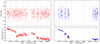 |
Fig. 1. Top panels: satellite-orbit averaged and reduced BRITE light curves for o Lupi, where the UBr photometry is indicated in red (left) and the BAb photometry in blue (right). Photometric variability is indicated in parts-per-thousand (ppt). Bottom panels: corresponding satellite-orbit averaged temporal variability of the on-board CCD temperature, showing different and discontinuous behavior. |
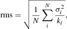
The final corrected, detrended, and satellite-orbit averaged photometry is given in Fig. 1. To assess the quality of the reduced BRITE photometry, we also provide the values for some diagnostic parameters in Table 1. The first of these parameters is the root mean square (rms) of the flux, given as
 (1)
(1)
Diagnostics related to the two BRITE light curves of o Lupi.
where σi and ki are the standard deviation of the flux and the number of observations within orbital passage i, respectively, and N is the total number of orbital passages for a given BRITE dataset. Also listed are the median duty cycle per satellite orbit Dorb and the fraction of successful satellite orbits Dsat. The former indicates the portion of the satellite orbit used for observations, while the latter parametrizes the amount of successful satellite orbits over the total time span of the light curve.
The two final BRITE light curves (UBr and BAb) formed the basis of the photometric analysis of the periodic variability of o Lupi discussed in Sect. 4.
2.2. Spectropolarimetry
The HARPSpol polarimeter (Piskunov et al. 2011) was employed in combination with the High Accuracy Radial velocity Planet Searcher (HARPS) spectrograph (Mayor et al. 2003) to measure the Zeeman signature indicating the presence of a large-scale magnetic field at the surface of o Lupi. This combined instrument is installed at the ESO 3.6 m telescope at La Silla Observatory (Chile) and covers the 3800–6900 Å wavelength region with an average spectral resolution of 110 000. Standard settings were used for the instrument, with bias, flat-field, and ThAr calibrations taken at the beginning and end of each night. In total, 36 spectropolarimetric sequences were obtained during three different observing runs, in May 2011, July 2012, and April 2016. The first two campaigns were part of the Magnetism In Massive Stars (MiMeS) survey (Wade et al. 2016), and the third observing run was performed for the BRITE spectropolarimetric survey (Neiner et al. 2017). Each spectropolarimetric sequence consists of four consecutive sub-exposures with a constant exposure time ranging between 207 s and 1000 s. An overview of the spectropolarimetric dataset is given in Table A.2.
The HARPSpol data were reduced using the REDUCE package (Piskunov & Valenti 2002; Makaganiuk et al. 2011), and resulted in a circular spectropolarimetric observation for each sequence. A minor update to the package enabled us to extract individual spectra for each sub-exposure of the spectropolarimetric sequence. The spectropolarimetric observations were normalized to unity continuum using an interactive spline fitting procedure (Martin et al. 2018). This normalization method was performed per spectral order to achieve a smooth overlap between consecutive spectral orders. For the spectroscopy employed in this work, only the spectral orders of interest, taken from the spectropolarimetric sub-exposures, were normalized with the same interactive procedure.
o Lupi was also observed twice with the Echelle SpectroPolarimetric Device for the Observation of Stars (ESPaDOnS, Donati et al. 2006) mounted at the Canada France Hawaii Telescope (CFHT) on Mauna Kea in Hawaii in April and June 2014 (PI: M. Shultz). These spectropolarimetric sequences comprise of four consecutive sub-exposures with an exposure time of 85 s. They span the 3700–10 500 Å wavelength region with an average resolving power of 65 000. The data were reduced with the LIBRE-ESPRIT (Donati et al. 1997) and UPENA softwares available at CFHT. The resulting ESPaDOnS spectropolarimetric and spectroscopic observations were normalized to unity continuum in the same manner and using the same interactive tool as for the HARPSpol data. Details for the ESPaDOnS spectropolarimetry are provided in Table A.2.
3. Comparison with synthetic spectra
An accurate magnetometric analysis (Sect. 5) starts from the appropriate spectral line pattern (also referred to as the line mask), which is defined by the atmospheric characteristics of the star. To this aim, we used a grid of synthetic spectra to model the observed Balmer lines (Hα, Hβ, Hγ, and Hδ) and selected helium and metal lines, deriving a value for the effective temperature, Teff, and the surface gravity, log g, of o Lupi. The selected lines included the He I 4471Å line and the Mg II 4481Å line, since their relative depths are good indicators for Teff and log g. The synthetic spectra produce a (good) first approximation of the stellar parameters, because the fainter secondary component and possible surface abundance inhomogeneities will lead to an uncertain chemical abundance analysis.
A model grid covering a range of Teff spanning from 3500 K to 55 000 K and log g from 0.00 dex to 5.00 dex2 was calculated using ATLAS9 model atmospheres by Bohlin et al. (2017; retrieved from the Mikulski Archive for Space Telescopes: MAST) and Martin et al. (2017) assuming plane parallel geometry, local thermodynamic equilibrium, and an opacity distribution function for solar abundances (Kurucz 1993). Synthetic spectra were computed with COSSAM_SIMPLE (Martin et al. 2017).
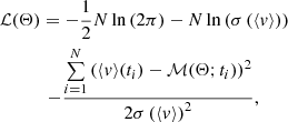
We varied the Teff and log g of the synthetic spectra, applying various values for the rotational broadening around the literature value of v sin i = 27 km s−1, and allowing for a radial velocity (RV) offset to fit the ESPaDOnS spectra. This resulted in a best fit with Teff = 15 000 K, log g = 3.8 dex, and v sin i = 35 km s−1. The wings of the Balmer lines are generally well described by the model, while the depths of the He I lines or several metal lines, such as those of Mg II, are overestimated. Peculiar surface abundances connected to the large-scale magnetic field can produce such a discrepancy since the grid relies on a solar composition for the synthetic data. We show the ESPaDOnS observations and the best synthetic model in Fig. 2, as well as the residuals to the fit.
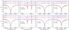 |
Fig. 2. Comparison between two ESPaDOnS spectra of o Lupi, taken two months apart (shown in gray), and synthetic ATLAS9/COSSAM_SIMPLE spectra. The red line is the synthetic spectrum for a single star with Teff = 15 000 K, log g = 3.8 dex, and v sin i = 35 km s−1, and the blue line is the synthetic spectrum for a binary star with Teff, 1 = 17 000 K, Teff, 2 = 14 000 K, log g1 = 3.9 dex, log g2 = 3.8 dex, v sin i1 = 50 km s−1, v sin i2 = 25 km s−1, RV1 = −5 km s−1, RV2 = +5 km s−1, and a light fraction of 50%. Residuals to the fit are indicated with the same color coding and a small offset for increased visibility. Top row: observed spectrum E01; bottom row: E02 (see also Table A.2). |
However, o Lupi is a known interferometric binary system. The contrast ratio derived by Rizzuto et al. (2013) implies that about 40% of the flux should originate from the secondary component. Moreover, the angular separation between the two components of o Lupi is sufficiently small that both fall within the fiber of modern spectrographs. However, the secondary has never firmly been detected in spectroscopy. Employing the ATLAS9 and COSSAM_SIMPLE synthetic spectra, we investigated whether a binary spectrum describes the observations better than a single star.
We varied Teff for both components from 13 000 K up to 18 000 K and log g from 3.5 dex up to 4.5 dex, allowing various v sin i values, light fractions from 0% up to 50%, and relative RV offsets up to 50 km s−1. The best fit occurs for Teff, 1 = 17 000 K, Teff, 2 = 14 000 K, log g1 = 3.9 dex, log g2 = 3.8 dex, v sin i1 = 50 km s−1, v sin i2 = 25 km s−1, RV1 = −5 km s−1, RV2 = +5 km s−1, and a light fraction of 50%. This model is indicated in Fig. 2. While the description of the helium and metal lines improved, the fit to the Balmer lines did not necessarily improve. The binarity has a similar effect on the metal lines as a surface under-abundance, which is often observed for magnetic early-type stars. Moreover, the light fraction of the secondary is higher than determined from interferometry, that is the fitting algorithm tries to obtain a better description for the (weaker) metal lines. For these reasons, we rejected the more complex model, where both stars contributed equally to the spectroscopic observations, and accepted the simpler model where only one star is visible. Further, we argue that if both components do contribute, we cannot distinguish between them in the spectroscopy due to their similar spectral types, small RV shifts, and expected chemical peculiarities. This is in agreement with the results of Sect. 5.1, where we show that the Zeeman signature spans the full width of the average line profiles. Therefore, we adopt Teff = 15 000 K and log g = 3.8 dex as the starting point for the magnetometric analysis.
Incorrect values for Teff or log g do impact the analysis of the longitudinal magnetic field as an inappropriate set of lines will be used in the determination of the average line profile in the magnetometric analysis. However, slight discrepancies between the adopted values and the real ones would only have a negligible impact, since the line depth in the line mask will be adjusted to the observations (see also Sect. 5.1).
4. Periodic photometric variability
Magnetic early-type stars often show periodic photometric variability due to co-rotating surface abundance inhomogeneities caused by the large-scale magnetic fields. Moreover, Alecian et al. (2011) discussed the possibility of stellar pulsations in o Lupi, yet attributed the LPVs to surface abundance inhomogeneities. To determine the cause of the LPVs, we investigated the BRITE photometry for coherent periodic variability. We employed an iterative prewhitening approach to determine the frequencies of the periodic variability. Following the spectroscopic results of Sect. 3, we attributed all photometric variability in the BRITE data to the primary component. However, implications and ambiguity caused by the binary system of o Lupi are further discussed in Sect. 7.
Iterative prewhitening is typically applied to recover and study the stellar pulsation mode frequencies of massive and early-type stars in both ground-based and space-based photometry (e.g., Degroote et al. 2009a). The method determines the most significant periodic variability, fits a (sinusoidal) model to the data with that frequency, calculates the residuals to the model, and iteratively continues this scheme to the residuals until no significant periodic variability remains. Adopting this approach, we searched for the significant frequencies in ten times oversampled Lomb-Scargle periodograms (Lomb 1976; Scargle 1982) of the BRITE photometry within the 0–8 d−1 frequency range. No variability was expected at higher frequencies. The significance of frequency peaks was calculated using the signal-to-noise (S/N) criterion (Breger et al. 1993) with a frequency window of 1 d−1 centered at the frequency of the variability and this after its extraction. Frequency peaks were considered significant if their S/N reached the threshold value of four. The periodograms for each BRITE light curve are shown in Fig. 3.
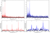 |
Fig. 3. Lomb-Scargle periodograms showing the periodic variability for the UBr (left panels) and BAb (right panels) light curves. Top panels: periodograms covering the full investigated frequency domain. The periodograms of the light curve are given in red (UBr; left) and blue (BAb; right), while the variability of the residuals after the iterative prewhitening is given in black. Bottom panels: periodograms covering the frequency domain where significant periodic variability is recovered. The amplitude of the periodic variability is given in parts-per-thousand (ppt). The frequencies of the extracted variability is given by the small black ticks in the top part of each panel. |
This method resulted in six significant frequencies for the UBr photometry and three frequencies for the BAb photometry, in the frequency domain of 0–1.5 d−1. We report these in Table 2, together with their respective uncertainties. It was expected that the analysis of the BAb would result in less clear periodic variability, represented by the smaller amount of significant frequencies, due to the large time gap, which complicated the analysis. We note that f2 is the second frequency harmonic of f1 and f5 is the third harmonic of f1, making it very likely that these three frequencies are related to the rotational modulation of the magnetic component. (We confirm this hypothesis in Sect. 5.) Moreover, f4 is very close to 1.0 d−1, which is a known instrumental frequency for the BRITE photometry, related to the periodic on-board temperature variability (e.g., Fig. A.4 of Buysschaert et al. 2017b). No significant amplitude changes were retrieved during the length of the BRITE light curves.
Significant periodic photometric variability seen in the UBr and BAb BRITE photometry of o Lupi.
Periodic variability with the same frequency in both the UBr and BAb photometry had comparable amplitudes (see Table 2). The frequencies f3 and f6 are likely due to a g-mode pulsations. In this case, the slightly higher amplitude for f3 in the blue filter was expected. Yet, without additional and simultaneous time resolved photometry employing different bandpass filters, performing mode identification of the stellar pulsations with the amplitude ratio method was impossible (see e.g., Handler et al. 2017; where this method was successfully applied for a pulsating early-type star with BRITE and ground-based photometry). As the retrieved variability had similar amplitudes, we ignored the colou = r information of the individual BRITE light curves and combined these into one light curve. This was done once without any weighting methods and once with a simple weighting method (using the rmscorr values) to account for differences in data quality, but overall no simple weighting method is available for BRITE photometry (see also Handler 2003; for more general information on possible weighting methods). Subsequent iterative prewhitening did not result in any new significant periodic variabilitycompared to what was already obtained from the UBr data.
Once all significant periodic photometric variability was subtracted from the UBr photometry, the frequency diagram of the residuals seems to be nearly constant with amplitudes well below 1 ppt (see Fig. 3). No obvious variability remained in the residual light curves in the time domain. Moreover, the noise level in the periodogram of the residual BAb photometry was considerably higher than that of the UBr residuals, because it has less data points.
5. Magnetic measurements
5.1. Zeeman signatures
To reliably detect the Zeeman signature of a stable large-scale magnetic field at the surface of an early-type star, mean line profiles are constructed from each high-resolution spectropolarimetric observation to boost the S/N of the signature in the Stokes V polarization. We employed the least-squares deconvolution (LSD) technique (Donati et al. 1997) to create these mean line profiles. We started from a pre-computed VALD3 line mask (Ryabchikova et al. 2015) with Teff = 15 000 K and log g = 4.0 dex, which is the closest match to our results Teff = 15 000 K and log g = 3.8 dex from the simpler model describing the spectroscopic observations (see Sect. 3 for a discussion between both used models). We removed from the line mask all hydrogen lines and all helium and metal lines that were blended with hydrogen lines, telluric features, and known diffuse interstellar bands to ensure we only included absorption lines with similar line profiles (the only exception being the He I lines where pressure broadening through the Stark effect is still significant). All metal lines with a depth smaller than 0.01 were also discarded. Lastly, the depths of the lines included in the line mask were adjusted to correspond to the observations (a technique sometimes referred to as “tweaking the line mask”, see e.g., Grunhut et al. 2017). This resulted in a final line mask with 893 lines included, each with their respective wavelength, line depth, and Landé factor. An additional line mask (and corresponding LSD profiles) without (blends with) He I lines was also constructed and included 821 metal lines. We show these mean line profiles in Fig. 4 for both line masks. The Zeeman signature in the LSD Stokes V profile clearly varies between the various observations. Moreover, the LSD Stokes I profile exhibits clear LPVs, possibly due to the rotational modulation caused by surface abundance inhomogeneities or the stellar pulsation. Fortunately, the diagnostic null profiles (i.e., deconstructively added polarization signal within the sequence, Donati et al. 1997) suggest that no significant instrumental effects or LPVs have occurred during the spectropolarimetric sequence, as they are flat.
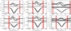 |
Fig. 4. Overplotted mean line profiles constructed with the LSD method using various line masks. From top to bottom panels: LSD Stokes V profile, diagnostic null profile, and LSD Stokes I profile for the observations, that are off-set for increased visibility. Differences in the line depth of the LSD Stokes I profile, the strength and shape of the Zeeman signature in the LSD Stokes V profile, and the shape of the LPVs in the LSD Stokes I profile are clearly visible. We indicate the integration limits for the computation of the longitudinal magnetic field and the FAP determination by the red dashed lines for each observation. For the Balmer lines, only the cores of the LSD Stokes I profiles were used and shifted upwards to unity, following the technique of Landstreet et al. (2015, see text). |
To determine whether an LSD Stokes V spectrum contained a Zeeman signature, we determined the False Alarm Probability (FAP; Donati et al. 1992, 1997) for each LSD profile. Definitive detections (DD) show a clear signature and correspond to a FAP < 10−3%, while non-detections (ND) have a FAP > 10−1%. Marginal detections (MD) fall in between DDs and NDs, with 10−3% < FAP < 10−1%. Based on these criteria, all LSD profiles indicated a DD, irrespective whether the complete line mask or the He-excluded line mask was used. Thus, a large-scale magnetic field is clearly detected in the high-resolution spectropolarimetry.
Figure 4 further indicates that the Zeeman signature in LSD Stokes V spans the full width of the LSD Stokes I profile, demonstrating that this full width corresponds to the magnetic component. No additional spectroscopic component is identified in the LSD Stokes I profiles. Since the interferometric results of Rizzuto et al. (2013) indicated that o Lupi is a binary system with a comparable light fraction, both components must have a similar spectral type and have small RV shifts. This, together with the presence of LPVs, makes it impossible to discern which component hosts the detected large-scale magnetic field. These results are in agreement with those from the spectroscopic analysis of Sect. 3. As such, we will likely underestimate the true strength of the magnetic field through an overestimated depth of the Stokes I profile in Eq. (2).
5.2. Longitudinal field measurements
Since the large-scale magnetic fields of early-type stars are expected to be stable over long timescales and inclined with respect to the rotation axis, the measured longitudinal magnetic field should exhibit rotational modulation (depending on the relative orientation to the observer). This rotational modulation can be used to accurately determine the rotation period of the magnetic component of o Lupi.
The longitudinal magnetic field (in Gauss, see Rees & Semel 1979) is measured as
![Mathematical equation: $$ \begin{aligned} B_l = -2.14 \times 10^{11} {\frac{\int { v} V({ v}) {\mathrm{d} }{ v}}{\lambda { g} c \int [1-I({ v})] {\mathrm{d} }{ v}}}, \end{aligned} $$](/articles/aa/full_html/2019/02/aa31913-17/aa31913-17-eq3.gif) (2)
(2)
where V(v) and I(v) are the LSD Stokes V and I profiles for a given velocity v. The parameters g, the mean Landé factor, and λ, the mean wavelength (in nm) come from the LSD method. The speed of light is given by c (in km s−1). We provide g and λ for the various line masks in Table 3 and the determined values for Bl in Table A.1. The integration limits to determine the Bl should cover the full LSD Stokes I profile, and thus, also the full Zeeman signature. Following the plateau method (e.g., Fig. 3 of Neiner et al. 2012), where we investigated the dependency of Bl and σ(Bl) with the integration limit for a near magnetic pole-on observation, we determined an integration range of ±65 km s−1 and ±60 km s−1 around the line centroid to be the most appropriate for the complete and the He-excluded LSD profiles, respectively. These values were considerably larger than the literature v sin i = 27 km s−1 for o Lupi, which did not capture the complete width of the absorption profile or the Zeeman signature due to the application of the LSD technique.
Parameters related to the study of the longitudinal field measurements from various LSD line masks.
When the large-scale magnetic field has a pure dipolar geometry, the rotational modulation of the measured longitudinal magnetic field can be characterized by a sine model:
 (3)
(3)
where B1 and ϕ1 are the amplitude and phase of the sine, B0 the constant offset, and frot the rotation frequency. However, when the large-scale magnetic field has a dipolar component with a non-negligible quadrupolar contribution, the longitudinal magnetic field modulation is given by a second-order sine model:
 (4)
(4)
Again, Bi and ϕi are the amplitude and phase of the individual sine terms. We fitted both models to the longitudinal magnetic field measurements of the He-excluded LSD profiles using a Bayesian Markov chain Monte Carlo (MCMC) method (using EMCEE; Foreman-Mackey et al. 2013) to determine the rotation period. We adopted the log-likelihood function for a weighted normal distribution:
 (5)
(5)
with ln the natural logarithm, ℳ(Θ; ti) the model of Eq. (3) or Eq. (4) for a given parameter vector Θ at timestep ti. The measured longitudinal magnetic field at ti is given by Bl(ti), its respective error by σ(Bl(ti)), and N is the number of observations. We constructed uniform priors in the appropriate parameter spaces for each free parameter describing the models of Eqs. (3) and (4). For the rotation frequency, this was around f1 from the BRITE photometry with a range set by the Rayleigh frequency criterion employing the time length of the spectropolarimetric dataset (fres = 0.0006 d−1). Calculations were started at random points within the uniform parameter space employing 128 parameter chains and continued until stable frequency solutions were reached.
The posterior probability distribution function (PDF; see Fig. 5) of the rotation frequency of Eq. (4) showed a maximum at frot = 0.338601(2) d−1, corresponding to a rotation period of Prot = 2.95333(2) d. Also the PDF for the amplitudes B1 and B2, and the offset B0 show a normal distribution centered at a non-zero value. The distributions for the phases ϕ1 and ϕ2 are nearly uniform, which is expected as frot was a free parameter during this process and each value of frot from the PDF creates a normal distribution for the phase ϕi. The superposition of these normal distributions for ϕi creates the obtained nearly uniform distribution. We indicate the recovered PDFs for the fitting parameters in Fig. 5 and list the deduced values for B0, B1, and B2, with their respective uncertainties, in Table 3. The fit to the Bl values computed from the He excluded LSD profile resulted in a non-zero value for B2, indicating that the second-order term of the model is needed, hence the quadrupolar component of the large-scale magnetic field is significant. This was further supported by the information criteria during the fitting process and model selection. Once a value for each fitted parameter was obtained, we defined an initial epoch T0 around the first observations (i.e., H01), to place the maximum of the (sine-model) at a rotation phase of 0.5.
 |
Fig. 5. Results of the MCMC analysis on the measured longitudinal magnetic field of the He-excluded LSD profiles using the model of Eq. (4). The posterior probability distributions (PDF) are indicated for each fitted parameter. When these had a normal distribution, we represent it with the Gaussian description marked in red. |
Assuming that both components of o Lupi contribute to the spectropolarimetric data and that their rotation periods are significantly shorter than the length of the spectropolarimetric time series, we assert that only one component hosts a strong large-scale magnetic field. Indeed, there is a lack of variability in the measured longitudinal magnetic field other than with a period Prot. A second magnetic component would severely distort the rotational modulation indicated in Fig. 6. Only a binary system with synchronized rotation periods could reproduce this variability, which is highly unlikely for the o Lupi binary system given its Porb > 20 years.
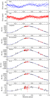 |
Fig. 6. Phase folded BRITE light curves (after subtracting the non-rotational variability; upper two panels) and longitudinal magnetic field measurements from LSD profiles with various line masks, using a Prot = 2.95333 d and T0 = HJD 2455702.5, and indicated by the observing campaign (black for MiMeS, red for BRITEpol, and green for ESPaDOnS). The pure dipole model for the geometry of the large-scale magnetic field of Eq. (3) is indicated by the dashed blue line and the dipole with a quadrupole contribution of Eq. (4) is indicated by the solid black line. Note the differences in strength of the measured Bl values for the various LSD line masks. |
We included the BRITE light curves, phase folded with Prot and the periodic variability not caused by the rotation removed, in Fig. 6 to compare the photometric rotational modulation with that of the longitudinal magnetic field. The peak brightness in the folded BRITE light curves occurs close to the phase where we observed the magnetic poles (at rotation phases 0.0 and 0.5), suggesting that the brighter surface abundance inhomogeneities are located close to the magnetic poles. The remaining photometric variability depends on the inclination angle i, the obliquity angle β, and the relative positions and sizes of the abundance inhomogeneities at the stellar surface, which requires tomographic imaging and/or spot modeling and is beyond reach of the current data.
5.3. Single-element longitudinal field measurements
While adjusting the line depths of the metal lines used in the LSD line masks, we noted that the Zeeman signature shows different strengths for different chemical species. Therefore, we constructed three different line masks containing only 19 He I, 264 Fe II, or 61 Si II metal lines. Special care was taken to exclude any line blends with metal lines that had a stronger or similar line depth than the considered chemical element. The corresponding mean Landé factors and mean wavelengths are given in Table 3, and the LSD profiles themselves are given in Fig. 4. Similar to the LSD profiles constructed with the complete line mask, we obtained DDs for all LSD profiles constructed with either Si II or Fe II lines. For the He I LSD profiles, however, we obtained ten NDs, and 26 DDs, most likely caused by the lower S/N, as fewer lines were included in constructing the mean line profile. Indeed, the S/N in the LSD Stokes V and Stokes I profiles of the He I line mask was typically three times lower than that of the Fe II LSD profiles (see Table A.2). Again, we noted strong LPVs for the LSD Stokes I profiles of all single-element LSD line masks, while the diagnostic null profiles indicated that no LPVs or instrumental effects have occurred during the spectropolarimetric sequence. We study these LPVs in more detail in Sect. 6.
We used the single-element LSD line masks to measure the longitudinal magnetic field associated with the large-scale magnetic field. Again, we employed the plateau method to determine the integration range for the computations. This resulted in an integration limit of 65 km s−1, 60 km s−1, and 60 km s−1 around the line centroid for the He I, Fe II, and Si II line masks, respectively. Keeping the rotation frequency fixed to the previously derived value, we performed a Bayesian MCMC fit to model the rotational modulation of the measured longitudinal magnetic field. These models and the measured values are shown in Fig. 6.
The rotational modulation of the measured Bl values from the LSD profiles constructed with only Fe II lines favored the model of a dipolar magnetic field with a quadrupolar contribution. This is in agreement with the results for the complete LSD line masks derived in Sect. 5.2. For the analysis of the measured longitudinal magnetic field of o Lupi with only Si II lines, we obtained a less clear distinction between both models for the rotational modulation of the measured Bl values. Both models agree with the measurements, within the derived uncertainties on the Bl values. Yet, the fit with the model of dipolar magnetic field and a quadrupolar component was preferred from the information criteria. Lastly, the Bl values measured from the He I LSD line mask were much smaller. This caused the rotational modulation of the measured Bl values to be minimal, leading to a comparable description by both models. Since the deduced errorbars on the measured Bl values for the He I remained comparable to those derived from the other LSD line masks, it seemed likely that the noted differences are (astro)physical. Surface abundance inhomogeneities structured to the geometry of the large-scale magnetic field at the stellar surface could be an explanation. Elements that are concentrated at the magnetic poles will lead to larger Bl values, while elements located close to the magnetic equator will result in smaller Bl values. Such features should be noted during tomographic analyses (i.e., Zeeman Doppler Imaging; ZDI), but require a spectropolarimetric dataset which is more evenly sampledover the rotation period than the current observations.
Finally, we tried to model the Zeeman signature of the large-scale magnetic field, seen in the LSD Stokes V profile, using a grid-based approach (see e.g., Alecian et al. 2008; for further details). However, we were not able to accurately model the changing Zeeman profile with varying rotation phase. This was likely caused by the insufficient sampling of the rotation phase at key phases.
5.4. Balmer lines longitudinal field measurements
The magnetometric analysis of single-element LSD profiles exhibited a strong scatter in the strength of the measured Bl values, suggesting surface abundance inhomogeneities for certain chemical elements (e.g., He, Si, and Fe). To measure the rotational modulation of the longitudinal magnetic field for an element that should be homogeneously distributed over the stellar surface we analyzed hydrogen lines. The wavelength regions around the Balmer lines in the spectropolarimetric observations were normalized with additional care, employing only linear polynomials, so as not to influence the depth of the line core or the broad wings.
We constructed a mean line profile for the Balmer lines, including Hα, Hβ, and Hγ in the LSD line mask. Three of these profiles indicated a ND and one a MD of a Zeeman signature in the observations, most likely due to the lower S/N in the Stokes V profiles for these observations. We then followed the method of Landstreet et al. (2015) to measure the Bl values. This method uses only the core of the line and ignores the broad wings. Moreover, to scale the measurements more in line with those from the metal lines, the (LSD) Stokes I profile was not integrated from unity, but instead from the intensity level, Ic, where the core transitions into the wings. As the Zeeman signature in the LSD Stokes V profile is slightly wider than the core of the Stokes I profile, we employed this width to set the integration range to 100 km s−1 around the Stokes I line centroid. We present these LSD profiles in Fig. 4, where the indicated Stokes I profile is shifted upwards to place Ic at unity. While fixing the rotation frequency, we performed a Bayesian MCMC fit to determine the fitting parameters for the description of the rotational modulation of the measured Bl values. The fit of both models to the measured Bl values is given in Fig. 6, with the parameters in Table 3.
The rotational modulation of the measured longitudinal magnetic field from the Balmer lines was more accurately represented by the model for a dipolar magnetic field and a quadrupolar component. This result agreed with those of the other LSD profiles. Yet, the discrepancies between this model and that of a dipolar magnetic field were small at most of the rotation phases, due to large uncertainties in Bl, caused by the low S/N in the LSD Stokes V profiles.
6. Line profile analysis
Pulsating early-type stars and magnetic early-type type stars are both known to exhibit LPVs. Alecian et al. (2011) already noted such behavior for o Lupi. Therefore, we investigated the zeroth and first moment of selected absorption lines for periodic variability employing the software package FAMIAS (Zima 2008). The analysis of six absorption lines, using the sub-exposures of the spectropolarimetric sequences, is presented in Sect. 6.1. We also investigated the Hα line for variability in Sect. 6.2, to try to diagnose the presence of a magnetosphere. Lastly, we examined the possibility of co-rotating surface abundance inhomogeneities by analyzing the zeroth moment of six absorption lines in Sect. 6.3.
6.1. Individual lines
To analyze the LPVs of stellar pulsations in absorption lines, it is preferred to work with deep and unblended absorption lines. This remains valid when investigating the signatures caused by the rotational modulation of surface abundance inhomogeneities. During the analysis of the Zeeman signature in the LSD Stokes V profile, we noted differences between different chemical species. Therefore, we selected absorption lines from various elements. For He, we selected and analyzed the He I 4713.2 Å and the He I 6678.2 Å lines, which are close multiplets of several He lines. In addition, the Mg II 4481.1 Å fulfilled the set criteria. At an effective temperature of 15 000 K, there are not many strong and suitable Si lines. Therefore, we opted for the Si II 6347.1 Å, although it is blended with the weaker Mg II 6347.0 Å line. Similarly, we selected the Fe II 4549.5 Å line, which blends with a weak Ti II line. Lastly, we chose the C II 4267.3 Å line, which is actually a multiplet. The spectroscopy employed during the LPV analysis was the individual sub-exposures of the spectropolarimetric sequences. We removed the last two sub-exposures of the observation H25 (see Table A.2), since they did not contain any flux due to bad weather. This resulted in a total of 142 spectroscopic observations taken over ∼1780 days, with large time gaps in between each observing campaign. We show the selected spectroscopic lines in Fig. 7, together with their mean line profile and the standard deviation of all observations of a given absorption line. The latter indicated a different shape for the LPVs for the Fe II and Si II lines compared to the other selected absorption lines, such as the He I or C II lines. This might indicate a different dominant variability, and hence a different origin or cause for the LPVs. The standard deviation of the selected Mg II line also looked slightly different, yet it seemed to be an intermediate profile between the two studied He I lines.
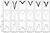 |
Fig. 7. LPVs for various selected absorption lines. Top panels: all observations of the given line overlayed to illustrate the LPVs. As an additional diagnostic, we indicate the mean profile (middle panels) and standard deviation (std; bottom panels) of all observations. The standard deviation, particularly, shows strong differences when comparing the selected absorption lines. |
For each line selected, we set appropriate limits for the calculation of their moments. These limits were set at similar flux levels for a given spectral line, close to the continuum level, unless strong pressure broadening (e.g., He I 6678.2 Å) or asymmetries in the line wings (e.g., C II 4267.3 Å) were noted, resulting in a more narrow range. We determined the zeroth, ⟨v0⟩, first, ⟨v⟩, and second moment, ⟨v2⟩, (representative of the equivalent width, radial velocity, and skewness, respectively) for each selected line with the software package FAMIAS (Zima 2008). Here we continue the discussion of the coherent periodic variability in the first moment. The zeroth moment is analyzed in Sect. 6.3. From the BRITE photometry and the rotational modulation of the longitudinal magnetic field, two phenomena were already known to cause periodic variability, each with a distinct period. These phenomena are rotation modulation (with Prot = 2.95333 d) and the dominant g-mode pulsation (with f3 = 1.1057 d−1). We constructed a model that included the (potential) periodic variability in the measured line moments:
 (6)
(6)
where Arot, i and Apuls are the amplitudes of the variability, ϕrot, i and ϕpuls their respective phases, and C a constant off-set. We deduced each free parameter with a Bayesian MCMC method. Uniform priors were assumed for all parameters in their appropriate parameter spaces, in particular fpuls had to agree with the conservative result of the BRITE photometry (i.e., f3 = 1.1057 ± 0.0070 d−1, where the Rayleigh frequency limit was assumed), and frot was kept fixed to the value from the magnetometric analysis. The quality of the fit was determined by the loglikelihood function for a (non-weighted) normal distribution:
 (7)
(7)
where σ(⟨v⟩) is the error on all ⟨v⟩, on the order of 1 km s−1. Again, 128 parameter chains were used during the MCMC fitting, starting from random positions within the uniform priors, and computations continued until stable solutions were reached. The computed values for the parameters in Eq. (6) and ℒ(Θ) are given in Table 4. Furthermore, we phase-folded ⟨v⟩ with the determined fpuls and with frot and show these in Fig. 8.
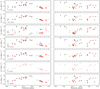 |
Fig. 8. Phase folded ⟨v⟩ for selected absorption lines with the average derived g-mode pulsation frequency (fpuls = 1.10573 d−1 and T0 = HJD 2455702.0; left; see Table 4) and the rotation period from the magnetometric analysis (Prot = 2.95333 d and T0 = HJD 2455702.5; right). The same colors were used to indicate the different observations as in Fig. 6. |
The derived amplitudes indicated that the rotational modulation and the dominant g-mode frequency cause the LPVs noted for the absorption lines. However, the contribution (i.e., the amplitude) of each variability term in ⟨v⟩ differed greatly when comparing the different absorption lines. Variability due to the stellar pulsation was dominant for the investigated C II, Mg II, and He I lines, while the LPVs in the Fe II line were due to the rotational modulation. Contributions to the periodic variability of ⟨v⟩ for the studied Si II line were almost equal. As such, the occurrence of surface abundance inhomogeneities only occurred for that particular chemical element, while LPVs due to the g-mode were always present. These observed features can also be seen in Fig. 8. Future tomographic analyses, such as ZDI, should indicate the distribution of the surface abundance inhomogeneities more clearly.
We also obtained a value for the pulsation mode frequency fpuls from the Bayesian MCMC fit to each first moment of each absorption line. Yet, not all obtained values for the g-mode frequency agreed within the same confidence interval, pointing to heteroscedasticity of the first moment measurements.
6.2. Balmer lines
Magnetic early-type stars can host a magnetosphere in their nearby circumstellar environment. The interactions of wind material with this magnetosphere could, cause rotationally modulated variability in certain spectroscopic lines, with emission features in Hα the easiest to identify. For o Lupi, we did not observe such emission profiles, however, we did note variability in the core of the Hα line. We thus repeated the analysis of the line moments, where we restricted their computation to the core of the line, fixing the integration limits where the broad line wing starts.
We performed the same analysis as for the other absorption lines for the cores of the Hα line of each complete spectropolarimetric sequence. The Bayesian MCMC fit indicated that we did not detect any rotational modulation in the ⟨v⟩ of Hα, because the Arot, i all agreed with zero. Therefore, we did not identify variability coming from the (potential) magnetosphere. Similar to the majority of the lines of the previous section, the MCMC fits indicated that the g-mode pulsation frequency is the dominant source for the LPVs. The significantly lower ℒ(Θ) for the fit to the core of Hα is the result of using only 36 spectropolarimetric sequences compared to the 142 spectroscopic observations.
6.3. Surface abundance inhomogeneities
The equivalent width or zeroth moment can be used as a first approximation to follow the change in the surface abundance of chemical species. This has been employed before to confirm the presence of co-rotating surface abundance inhomogeneities for magnetic stars (e.g., Mathys 1991). We repeated the analysis of Sect. 6.1 by replacing ⟨v⟩ by ⟨v0⟩ in Eq. (6) and performing the Bayesian MCMC fit to the ⟨v0⟩ measurements. The determined amplitudes and ℒ(Θ) are provided in Table 4.
For each fit to the ⟨v0⟩ measurements of the different absorption lines, we obtained a value for Apuls compatible with zero. Moreover, the resulting PDFs for fpuls were flat. These results indicated that the g-mode does not cause any significant periodic variability in the ⟨v0⟩ measurements. This was expected, as most (non-radial) pulsation modes distort the shape of the line instead of altering the equivalent width. Furthermore, the fit to the measurements from the He I lines and Hα suggested that their abundances did not vary with the rotation period. For the remaining four studied lines, some degree of periodic variability with frot was deduced. We phase fold the ⟨v0⟩ measurements with frot and
show these in Fig. 9.
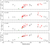 |
Fig. 9. Phase folded ⟨v0⟩ for absorption lines, for which non-zero values for Arot, i were derived, with the rotation period (Prot = 2.95333 d and T0 = HJD 2455702.5). The same colors were used to indicate the different observations as in Fig. 6. |
The variability of ⟨v0⟩ of the Fe II line can be described by a second order sine function (see also Table 4), but heavily relies on the scarce measurements between rotation phase 0.20 and 0.35. Moreover, the phase folded ⟨v0⟩ of the Fe II line seems to be coherent with the phase folded BRITE photometry (see top panels of Fig. 6). The simplest explanation for the LPVs in this Fe line, thus, is the presence of surface abundance inhomogeneities that are located close to the magnetic poles. Such a geometrical configuration agrees with the stronger measured longitudinal magnetic field from LSD profiles with only Fe lines (Fig. 6) and is often encountered for magnetic Ap/Bp stars (an example for the alignment between the large-scale magnetic field and (He) surface abundance inhomogeneities is presented in Oksala et al. 2018).
A different profile was obtained for the rotational modulation of the ⟨v0⟩ of the Si II line for which only a sinusoid was needed to capture the periodic variability (see Table 4). We recall that the amplitudes of the variability caused by the g-mode frequency and the rotational modulation of ⟨v⟩ measurements for this Si II line were comparable. These results indicate that the Si surface abundance inhomogeneities have a different location on the surface of o Lupi than the Fe surface abundance inhomogeneities. Because of the simple variation of ⟨v0⟩, we argue that we only observe one surface abundance inhomogeneity close to the magnetic equator.
For the two remaining absorption lines (i.e., C II and Mg II lines), the measured ⟨v0⟩ followed a profile in between that of the Fe II line and the Si II line, albeit with a smaller amplitude. The measured abundances of these lines are most likely following the changes in the local atmosphere caused by the Si and Fe surface abundance inhomogeneities.
7. Discussion
Comparison between the ESPaDOnS spectroscopy and synthetic spectra did not indicate o Lupi was an SB2 system, despite the interferometric results (Rizzuto et al. 2013). Either the secondary component is not visible in the spectroscopy, or the RV shifts were too small to detect due to two components of similar spectral type. Therefore, we continue this section under the assumption that only the primary component contributes to the variability and the large-scale magnetic field. We do comment, where applicable, what the implication would be in case of an indistinguishable secondary component in the spectropolarimetric or photometric data.
7.1. Geometry of the magnetic field
The rotational modulation of the measured longitudinal magnetic field favored the model a dipolar magnetic field with a quadrupolar contribution. The strength of the quadrupolar term in the model varied with the employed LSD line mask, but it was typically about 10% of the strength of the dipolar term (see Table 3).
Assuming a typical stellar radius of 3–4 R⊙ for a B5IV star with Teff = 15 000 K (e.g., Fig. 1 of Pápics et al. 2017) and employing the measured rotation period of 2.95333(2) d−1 and the literature v sin i = 27 ± 3 km s−1 (Głȩbocki et al. 2005), we estimated the inclination angle to be 27 ± 10° (corresponding to an equatorial velocity of veq = 60 ± 9 km s−1). These assumptions lead to an obliquity angle  , following the scaling relation of Shore (1987) for a purely dipolar large-scale magnetic field. The quadrupolar contribution needed for the description of the modulated longitudinal magnetic field will only have a minor effect on this estimated value. Moreover, this value does not depend strongly on the LSD line mask used for the measurements of the longitudinal magnetic field.
A conservative lower limit for the polar strength of the large-scale magnetic field (when the geometry is a pure dipole) is 3.5 times the maximal measured longitudinal magnetic field value (Preston 1967). Using the measurements of the LSD profiles from the Balmer lines, we obtained a lower limit of 5.25 kG for the polar strength of the magnetic field, since these were not influenced by the surface distribution of the chemical elements. This value is typical for magnetic Bp stars.
Detailed modeling of the Zeeman signatures or successful ZDI mapping of the stellar surface is required to verify the values derived from simple assumptions. However, the current spectropolarimetric dataset is not sufficient to do so, because of missing observations at several key rotation phases.
In case the secondary component significantly contributes to the spectropolarimetric data, which was not confirmed at present, we underestimated the strength of the detected large-scale magnetic field, since the total Stokes I profile was used for the normalization of the Bl values. For a 40% contribution of a secondary, the actual strength of the magnetic field will be underestimated by 40% or 60%, depending on which component is hosting the large-scale magnetic field.
We consider it unlikely that both components of the o Lupi binary system host a large-scale magnetic field with the published light ratio and the similar values for v sin i. In case both hosted a large-scale magnetic field, the similar light contributions would lead to two overlapping Zeeman signatures in the LSD Stokes V profiles, resembling a highly complex magnetic field geometry. The similar values for the v sin i (and light ratio) would suggest a similar rotation period, causing the longitudinal magnetic field to vary with two superimposed periods. This would lead to a strong beating effect. None of the above was observed (see Figs. 4 and 6). Only if both stars would rotate with exactly the same period could they pollute the observations unnoticed, and perhaps result in the necessity of the high-order fit to the measured Bl values. However, the synchronization timescale of a binary system with an orbital period of at least 20 years is sufficiently long to exclude this possibility.
7.2. Discrepancies in the measured magnetic field strength
Strong differences in the strength of the measured longitudinal magnetic field from different chemical elements are not often noted for magnetic early-type stars. They are, however, observed here. Surface abundance inhomogeneities are likely the cause of these differences. We support this hypothesis with the analysis of the LPVs, since the chemical species having a stronger longitudinal magnetic field are also the same species that indicated the rotation frequency as the dominant variability for the first moment (i.e., Fe II). Moreover, the zeroth moment of some studied absorption lines suggested that the measured equivalent width changes with the rotation phase, implying a non-uniform surface distribution for these chemical elements. A similar conclusion was obtained by Yakunin et al. (2015) for the magnetic helium-strong B2V star HD 184927. The larger measured Bl values for LSD profiles with just Fe II lines would indicate that their surface abundance inhomogeneities are located close to the magnetic pole, while the weaker fields retrieved from the He I would locate their respective surface abundance inhomogeneities close to the magnetic equator. In addition, the weaker longitudinal magnetic field measurements for the He I lines could also be related to a contribution in the LSD Stokes I profile coming from the secondary of the o Lupi system, which is suggested to have a similar spectral type.
We do not anticipate that the stellar pulsation is causing these severe differences in the measured longitudinal magnetic field strength. It would rather produce additional systematic offsets out of phase with the rotation period, as the pulsation frequency is not a harmonic of the rotation frequency. For the secondary component to cause these differences, it must have a different spectral type, leading to different contributions to spectral lines of different chemical species. This is in contradiction to the binary fitting process, that suggested a similar spectral type for both components. Also, the interferometric results indicated a relatively similar spectral type for the secondary and a mass ratio of 0.91 (Rizzuto et al. 2013).
7.3. Magnetosphere
The detected large-scale magnetic field for the primary component of o Lupi is sufficiently strong to create a magnetosphere. However, the star is not sufficiently massive to have a considerable mass-loss rate, producing only a limited amount of wind material to fill the magnetosphere. Therefore, no observational evidence of the magnetosphere is anticipated. Indeed, no rotational modulation, nor emission features were noted for the Balmer lines. No X-ray observations are available for o Lupi to diagnose the interactions between wind material coming from both magnetic hemispheres.
Petit et al. (2013) determined the star may host a centrifugal magnetopshere, using the magnetic properties derived by Alecian et al. (2011). Repeating these computations for a 4.7 M⊙ star with a 3.5 R⊙ radius, the updated Prot = 2.9533 d, and a polar magnetic field strength of 5.25 kG (and assuming a mass-loss rate described by Vink et al. 2001), we obtained RK = 4.2 R⋆ and RA = 26.5 R⋆ (and a mass-loss rate log Ṁ = −10.42 dex with Ṁ given in M⊙ yr−1). This confirms the results of Petit et al. (2013) that the magnetic component of o Lupi hosts a centrifugal magnetosphere. Yet, as previously indicated, the mass-loss rate is too low, particularly compared to the extend of the magnetosphere (RA ≫ RK), to produce observational evidence of magnetospheric material. In addition, the binary orbit of o Lupi is too wide to cause effects in the circumstellar material of the magnetic component.
7.4. Stellar pulsations
The BRITE photometry indicated that two frequencies, namely f3 = 1.1057 d−1 and f6 = 1.2985 d−1, were not explained as a frequency harmonic of the rotation frequency or as instrumental variability due to the spacecraft. Furthermore, we recovered f3 as the dominant periodicity in the first moment of the C II 4267.3 Å, Mg II 4481.1 Å, He I 4713.2 Å, and the He I 6678.2 Å lines, as well as from the core of Hα. The frequency value and the stellar parameters of the primary suggest that this frequency is a g mode. The majority of stars exhibiting such pulsation modes show a rich frequency spectrum, with sectoral dipole modes that are quasi-constantly spaced in the period domain (e.g., Pápics et al. 2014, 2017; Kallinger et al. 2017). We only find two pulsation mode frequencies due to the limited BRITE and ground-based data sets compared to the Kepler capacity in terms of aliasing.
The standard deviation of the lines (see Fig. 7) can serve as a proxy for the amplitude distribution from the pixel-by-pixel method (e.g., Gies & Kullavanijaya 1988; Telting & Schrijvers 1997; Zima 2006) in case one dominant periodicity causes the LPVs. As such, the shape of these distributions for the absorption lines that were dominantly variable with f3 suggested a low-degree mode (likely a dipole mode). Yet, detailed mode identification with FAMIAS did not produce conclusive results on the mode geometry. Furthermore, the frequency f6 = 1.2985 d−1 was also within the appropriate frequency domain for g-mode pulsations. In the absence of the secondary in the spectroscopy, we assumed that the g-mode pulsations originate from the magnetic component, as the majority of the LPVs were explained by f3. However, if the secondary contributed to the total flux, the periodic variability with f3 or f6 could be produced by the companion since its anticipated similar spectral type would place it within the SPB instability strip as well.
Without at least several detected pulsation modes, the magnetic and pulsating component of o Lupi is not a suitable candidate for magneto-asteroseismology, and so does not provide the opportunity to investigate the influence of the large-scale magnetic field on the structure and evolution of the stellar interior.
8. Summary and conclusions
We combined HARPSpol and ESPaDOnS spectropolarimetry to study and characterize the large-scale magnetic field of o Lupi. Using the variability of the measured longitudinal magnetic field, we determined the rotation period to be Prot = 2.95333(2) d, which agrees with earlier estimates that the rotation period would be on the order of a few days (Alecian et al. 2011). We assumed that the primary component of the o Lupi system hosts the large-scale magnetic field, given the lack of firm detection of a secondary component in the spectroscopy.
Comparing the strength of the measured Bl for various chemical elements, we noted large differences, indicative of chemical peculiarity and abundance structures at the stellar surface. The largest values were obtained for Fe, while the smallest values were derived from He I lines. This suggests that Fe surface abundance inhomogeneities are located closer to the magnetic poles, while those for He are present near the magnetic equator. Yet, we cannot fully exclude a possible contamination by the secondary component of o Lupi in the LSD Stokes I profiles. ZDI is needed to verify the locations of the suggested surface abundance inhomogeneities. Yet, this is not feasible with the current spectropolarimetric dataset, as we are lacking observations at several necessary rotational phases.
Fitting models to the rotational variability of the measured Bl values favors a description of a dipolar magnetic field with a quadrupolar contribution. This remains valid for the LSD profiles constructed with all metal lines, averaging out the effects of the surface abundance inhomogeneities, as well as for the LSD profiles from the Balmer lines. Typically, the strength of the quadrupolar contribution is about 10% of that of the dipolar contribution. Using simple approximations, we estimated the inclination angle of the magnetic component of o Lupi to be i = 27 ± 10°, which then leads to an obliquity angle  . A conservative lower limit on the polar strength of the large-scale magnetic field, measured from the LSD profiles of the Balmer lines, would be 5.25 kG.
The BRITE photometry for o Lupi shows up to six significant frequencies, indicating periodic photometric variability. Three of these frequencies (f1, f2, and f3) correspond to the rotation frequency, and its second and third frequency harmonic. One frequency (f4) is confirmed to be of instrumental origin, due to periodic variability of the satellite on-board temperature that was not perfectly accounted for during the correction process. The remaining two frequencies (f3 and f6) fall in the frequency domain of SPB pulsations. In case f3 and f6 originate from the magnetic component, o Lupi A would be classified as a magnetic pulsating early-type star. However, the few detected pulsation mode frequencies are not sufficient for detailed magneto-asteroseismic modeling.
Investigating selected absorption lines in the individual sub-exposures of the spectropolarimetric sequences indicates the presence of LPVs. The first moment of these absorption lines almost always indicate f3 as the dominant frequency, except for the Fe II line where frot was the dominant frequency. This is, again, suggestive of surface abundance inhomogeneities for Fe. Moreover, the equivalent width of the studied Fe II and Si II lines did change significantly with the rotation phase, demonstrating non-uniform surface abundances for these chemical species. The shape of the LPVs for the other selected absorption lines, where f3 was dominant, agreed with a low-order pulsation mode, confirming that f3 is a pulsation mode frequency.
As Teff increases, the range of the log g values covered reduces to values between 4.00 dex and 4.75 dex at 55 000 K.
Acknowledgments
This work was based on data gathered with HARPS installed on the 3.6 m ESO telescope (ESO Large Program 187.D-0917 and ESO Normal Program 097.D.0156) at La Silla, Chile and on observations obtained at the Canada-France-Hawaii Telescope (CFHT) which is operated by the National Research Council of Canada, the Institut National des Sciences de l’Univers of the Centre National de la Recherche Scientifique of France, and the University of Hawaii. Mode identification results obtained with the software package FAMIAS developed in the framework of the FP6 European Coordination Action HELAS (http://www.helas-project.eu). Based on data collected by the BRITE Constellation satellite mission, designed, built, launched, operated and supported by the Austrian Research Promotion Agency (FFG), the University of Vienna, the Technical University of Graz, the Canadian Space Agency (CSA), the University of Toronto Institute for Aerospace Studies (UTIAS), the Foundation for Polish Science & Technology (FNiTP MNiSW), and National Science Centre (NCN). B.B. thanks the participants of the third BRITE science workshop and the third BRITE spectropolarimetric workshop for the constructive comments on the presented work. In particular, Oleg Kochukhov for his suggestion to analyze the zeroth moment in more detail. This work has made use of the VALD database, operated at Uppsala University, the Institute of Astronomy RAS in Moscow, and the University of Vienna. This research has made use of the SIMBAD database operated at CDS, Strasbourg (France), and of NASA’s Astrophysics Data System (ADS). Some of the data presented in this paper were obtained from the Mikulski Archive for Space Telescopes (MAST). STScI is operated by the Association of Universities for Research in Astronomy, Inc., under NASA contract NAS5-26555. Support for MAST for non-HST data is provided by the NASA Office of Space Science via grant NNX09AF08G and by other grants and contracts. A. T. acknowledges the support of the Fonds Wetenschappelijk Onderzoek – Vlaanderen (FWO) under the grant agreement G0H5416N (ERC Opvangproject). The research leading to these results has (partially) received funding from the European Research Council (ERC) under the European Union’s Horizon 2020 research and innovation program(grant agreement N°670519: MAMSIE) and from the Belgian Science Policy Office (Belspo) under ESA/PRODEX grant “PLATO mission development”.
References
- Aerts, C., Símon-Díaz, S., Bloemen, S., et al. 2017, A&A, 602, A32 [NASA ADS] [CrossRef] [EDP Sciences] [Google Scholar]
- Aerts, C., Bowman, D. M., Símon-Díaz, S., et al. 2018, MNRAS, 476, 1234 [NASA ADS] [CrossRef] [Google Scholar]
- Alecian, E., Catala, C., Wade, G. A., et al. 2008, MNRAS, 385, 391 [NASA ADS] [CrossRef] [Google Scholar]
- Alecian, E., Kochukhov, O., Neiner, C., et al. 2011, A&A, 536, L6 [NASA ADS] [CrossRef] [EDP Sciences] [Google Scholar]
- Bigot, L., Provost, J., Berthomieu, G., Dziembowski, W. A., & Goode, P. R. 2000, A&A, 356, 218 [NASA ADS] [Google Scholar]
- Biront, D., Goossens, M., Cousens, A., & Mestel, L. 1982, MNRAS, 201, 619 [NASA ADS] [CrossRef] [EDP Sciences] [Google Scholar]
- Bohlin, R. C., Mészáros, S., Fleming, S. W., et al. 2017, AJ, 153, 234 [NASA ADS] [CrossRef] [Google Scholar]
- Breger, M., Stich, J., Garrido, R., et al. 1993, A&A, 271, 482 [NASA ADS] [Google Scholar]
- Briquet, M., Neiner, C., Aerts, C., et al. 2012, MNRAS, 427, 483 [NASA ADS] [CrossRef] [Google Scholar]
- Browning, M. K., Brun, A. S., & Toomre, J. 2004, ApJ, 601, 512 [NASA ADS] [CrossRef] [Google Scholar]
- Buysschaert, B., Neiner, C., Briquet, M., & Aerts, C. 2017a, A&A, 605, A104 [NASA ADS] [CrossRef] [EDP Sciences] [Google Scholar]
- Buysschaert, B., Neiner, C., Richardson, N. D., et al. 2017b, A&A, 602, A91 [NASA ADS] [CrossRef] [EDP Sciences] [Google Scholar]
- Buysschaert, B., Aerts, C., Bowman, D. M., et al. 2018, A&A, 616, A148 [NASA ADS] [CrossRef] [EDP Sciences] [Google Scholar]
- Degroote, P., Briquet, M., Catala, C., et al. 2009a, A&A, 506, 111 [NASA ADS] [CrossRef] [EDP Sciences] [Google Scholar]
- Degroote, P., Aerts, C., Ollivier, M., et al. 2009b, A&A, 506, 471 [NASA ADS] [CrossRef] [EDP Sciences] [Google Scholar]
- Donati, J.-F., Semel, M., & Rees, D. E. 1992, A&A, 265, 669 [NASA ADS] [Google Scholar]
- Donati, J.-F., Semel, M., Carter, B. D., Rees, D. E., & Collier Cameron, A. 1997, MNRAS, 291, 658 [NASA ADS] [CrossRef] [MathSciNet] [Google Scholar]
- Donati, J.-F., Catala, C., Landstreet, J. D., & Petit, P. 2006, in Solar Polarization 4, eds. R. Casini, & B. W. Lites, ASP Conf. Ser., 358, 362 [Google Scholar]
- Dziembowski, W., & Goode, P. R. 1985, ApJ, 296, L27 [NASA ADS] [CrossRef] [Google Scholar]
- Dziembowski, W. A., & Goode, P. R. 1996, ApJ, 458, 338 [NASA ADS] [CrossRef] [Google Scholar]
- Ferraro, V. C. A. 1937, MNRAS, 97, 458 [Google Scholar]
- Finsen, W. S. 1951, Circular of the Union Observatory Johannesburg, 112, 94 [NASA ADS] [Google Scholar]
- Foreman-Mackey, D., Hogg, D. W., Lang, D., & Goodman, J. 2013, PASP, 125, 306 [CrossRef] [Google Scholar]
- Gies, D. R., & Kullavanijaya, A. 1988, ApJ, 326, 813 [NASA ADS] [CrossRef] [Google Scholar]
- Głȩbocki, R., & Gnaciński, P. 2005, in 13th Cambridge Workshop on Cool Stars, Stellar Systems and the Sun, eds. F. Favata, G. A. J. Hussain, & B. Battrick, ESA SP, 560, 571 [Google Scholar]
- Goode, P. R., & Thompson, M. J. 1992, ApJ, 395, 307 [NASA ADS] [CrossRef] [Google Scholar]
- Gough, D. O., & Taylor, P. P. 1984, Mem. Soc. Astron. It., 55, 215 [NASA ADS] [Google Scholar]
- Gough, D. O., & Thompson, M. J. 1990, MNRAS, 242, 25 [Google Scholar]
- Grunhut, J. H., Wade, G. A., Neiner, C., et al. 2017, MNRAS, 465, 2432 [NASA ADS] [CrossRef] [Google Scholar]
- Handler, G. 2003, Balt. Astron., 12, 253 [NASA ADS] [Google Scholar]
- Handler, G., Shobbrook, R. R., Uytterhoeven, K., et al. 2012, MNRAS, 424, 2380 [NASA ADS] [CrossRef] [Google Scholar]
- Handler, G., Rybicka, M., Popowicz, A., et al. 2017, MNRAS, 464, 2249 [NASA ADS] [CrossRef] [Google Scholar]
- Hasan, S. S., Zahn, J.-P., & Christensen-Dalsgaard, J. 2005, A&A, 444, L29 [NASA ADS] [CrossRef] [EDP Sciences] [Google Scholar]
- Hubeny, I., & Lanz, T. 2011, Astrophysics Source Code Library [record ascl:1109.022] [Google Scholar]
- Kallinger, T., Weiss, W. W., Beck, P. G., et al. 2017, A&A, 603, A13 [NASA ADS] [CrossRef] [EDP Sciences] [Google Scholar]
- Kurucz, R. 1993, Opacities for Stellar Atmospheres: [+0.0],[+0.5],[+1.0]. Kurucz CD-ROM No. 2 (Cambridge, MA: Smithsonian Astrophysical Observatory) [Google Scholar]
- Landstreet, J. D., Bagnulo, S., Valyavin, G. G., et al. 2015, A&A, 580, A120 [NASA ADS] [CrossRef] [EDP Sciences] [Google Scholar]
- Lanz, T., & Hubeny, I. 2007, ApJS, 169, 83 [CrossRef] [Google Scholar]
- Lecoanet, D., Vasil, G. M., Fuller, J., Cantiello, M., & Burns, K. J. 2017, MNRAS, 466, 2181 [NASA ADS] [CrossRef] [Google Scholar]
- Lomb, N. R. 1976, Ap&SS, 39, 447 [Google Scholar]
- Makaganiuk, V., Kochukhov, O., Piskunov, N., et al. 2011, A&A, 525, A97 [NASA ADS] [CrossRef] [EDP Sciences] [Google Scholar]
- Martin, A. J., Stift, M. J., Fossati, L., et al. 2017, MNRAS, 466, 613 [NASA ADS] [CrossRef] [Google Scholar]
- Martin, A. J., Neiner, C., Oksala, M. E., et al. 2018, MNRAS, 475, 1521 [NASA ADS] [CrossRef] [Google Scholar]
- Mathis, S., & de Brye, N. 2011, A&A, 526, A65 [NASA ADS] [CrossRef] [EDP Sciences] [Google Scholar]
- Mathis, S., & Zahn, J.-P. 2005, A&A, 440, 653 [NASA ADS] [CrossRef] [EDP Sciences] [Google Scholar]
- Mathis, S., Neiner, C., & Tran Minh, N. 2014, A&A, 565, A47 [NASA ADS] [CrossRef] [EDP Sciences] [Google Scholar]
- Mathys, G. 1991, A&AS, 89, 121 [NASA ADS] [Google Scholar]
- Mayor, M., Pepe, F., Queloz, D., et al. 2003, The Messenger, 114, 20 [NASA ADS] [Google Scholar]
- Mestel, L. 1999, Stellar magnetism (Oxford) [Google Scholar]
- Montgomery, M. H., & O’Donoghue, D. 1999, Delta Scuti Star Newslett., 13, 28 [Google Scholar]
- Morel, T., Castro, N., Fossati, L., et al. 2015, in New Windows on Massive Stars, eds. G. Meynet, C. Georgy, J. Groh, & P. Stee, IAU Symp., 307, 342 [NASA ADS] [Google Scholar]
- Moss, D. 1989, MNRAS, 236, 629 [NASA ADS] [Google Scholar]
- Moss, D. 1992, MNRAS, 257, 593 [NASA ADS] [Google Scholar]
- Neiner, C., Alecian, E., Briquet, M., et al. 2012, A&A, 537, A148 [NASA ADS] [CrossRef] [EDP Sciences] [Google Scholar]
- Neiner, C., Mathis, S., & Alecian, E. 2015, in Polarimetry, eds. K. N. Nagendra, S. Bagnulo, R. Centeno, & M. Jesús Martínez González, IAU Symp., 305, 61 [Google Scholar]
- Neiner, C., Wade, G. A., Marsden, S. C., & Blazère, A. 2017, Polish Astron. Soc., 5, 86 [Google Scholar]
- Oksala, M. E., Silvester, J., Kochukhov, O., et al. 2018, MNRAS, 473, 3367 [NASA ADS] [Google Scholar]
- Pablo, H., Whittaker, G. N., Popowicz, A., et al. 2016, PASP, 128, 125001 [NASA ADS] [CrossRef] [Google Scholar]
- Pápics, P. I., Moravveji, E., Aerts, C., et al. 2014, A&A, 570, A8 [NASA ADS] [CrossRef] [EDP Sciences] [Google Scholar]
- Pápics, P. I., Tkachenko, A., Van Reeth, T., et al. 2017, A&A, 598, A74 [NASA ADS] [CrossRef] [EDP Sciences] [Google Scholar]
- Petit, V., Owocki, S. P., Wade, G. A., et al. 2013, MNRAS, 429, 398 [NASA ADS] [CrossRef] [Google Scholar]
- Piskunov, N. E., & Valenti, J. A. 2002, A&A, 385, 1095 [NASA ADS] [CrossRef] [EDP Sciences] [Google Scholar]
- Piskunov, N., Snik, F., Dolgopolov, A., et al. 2011, The Messenger, 143, 7 [NASA ADS] [Google Scholar]
- Popowicz, A., Pigulski, A., Bernacki, K., et al. 2017, A&A, 605, A26 [NASA ADS] [CrossRef] [EDP Sciences] [Google Scholar]
- Press, W. H. 1981, ApJ, 245, 286 [NASA ADS] [CrossRef] [Google Scholar]
- Preston, G. W. 1967, ApJ, 150, 547 [NASA ADS] [CrossRef] [Google Scholar]
- Rees, D. E., & Semel, M. D. 1979, A&A, 74, 1 [NASA ADS] [Google Scholar]
- Rizzuto, A. C., Ireland, M. J., & Robertson, J. G. 2011, MNRAS, 416, 3108 [NASA ADS] [CrossRef] [Google Scholar]
- Rizzuto, A. C., Ireland, M. J., Robertson, J. G., et al. 2013, MNRAS, 436, 1694 [NASA ADS] [CrossRef] [Google Scholar]
- Rogers, T. M., Lin, D. N. C., McElwaine, J. N., & Lau, H. H. B. 2013, ApJ, 772, 21 [NASA ADS] [CrossRef] [Google Scholar]
- Ryabchikova, T., Piskunov, N., Kurucz, R. L., et al. 2015, PhyS, 90, 054005 [Google Scholar]
- Scargle, J. D. 1982, ApJ, 263, 835 [Google Scholar]
- Shibahashi, H., & Takata, M. 1993, PASJ, 45, 617 [NASA ADS] [Google Scholar]
- Shore, S. N. 1987, AJ, 94, 731 [NASA ADS] [CrossRef] [Google Scholar]
- Simón-Díaz, S., Aerts, C., Urbaneja, M. A., et al. 2018, A&A, 612, A40 [NASA ADS] [CrossRef] [EDP Sciences] [Google Scholar]
- Spruit, H. C. 1999, A&A, 349, 189 [NASA ADS] [Google Scholar]
- Takata, M., & Shibahashi, H. 1995, PASJ, 47, 219 [NASA ADS] [Google Scholar]
- Telting, J. H., & Schrijvers, C. 1997, A&A, 317, 723 [NASA ADS] [Google Scholar]
- Tkachenko, A., Degroote, P., Aerts, C., et al. 2014, MNRAS, 438, 3093 [NASA ADS] [CrossRef] [Google Scholar]
- Townsend, R. H. D., & Owocki, S. P. 2005, MNRAS, 357, 251 [NASA ADS] [CrossRef] [MathSciNet] [Google Scholar]
- ud-Doula, A., & Owocki, S. P. 2002, ApJ, 576, 413 [NASA ADS] [CrossRef] [Google Scholar]
- Vink, J. S., de Koter, A., & Lamers, H. J. G. L. M. 2001, A&A, 369, 574 [NASA ADS] [CrossRef] [EDP Sciences] [Google Scholar]
- Wade, G. A., Neiner, C., Alecian, E., et al. 2016, MNRAS, 456, 2 [NASA ADS] [CrossRef] [Google Scholar]
- Weiss, W. W., Rucinski, S. M., Moffat, A. F. J., et al. 2014, PASP, 126, 573 [NASA ADS] [CrossRef] [Google Scholar]
- Yakunin, I., Wade, G., Bohlender, D., et al. 2015, MNRAS, 447, 1418 [NASA ADS] [CrossRef] [Google Scholar]
- Zahn, J. P. 2011, IAU Symp., 272, 14 [Google Scholar]
- Zima, W. 2006, A&A, 455, 227 [NASA ADS] [CrossRef] [EDP Sciences] [Google Scholar]
- Zima, W. 2008, Commun. Asteroseismol., 155, 17 [Google Scholar]
Appendix A: Additional tables
Overview of the measured longitudinal magnetic field values.
Observing log of the spectropolarimetric sequences.
All Tables
Significant periodic photometric variability seen in the UBr and BAb BRITE photometry of o Lupi.
Parameters related to the study of the longitudinal field measurements from various LSD line masks.
All Figures
|
Fig. 1. Top panels: satellite-orbit averaged and reduced BRITE light curves for o Lupi, where the UBr photometry is indicated in red (left) and the BAb photometry in blue (right). Photometric variability is indicated in parts-per-thousand (ppt). Bottom panels: corresponding satellite-orbit averaged temporal variability of the on-board CCD temperature, showing different and discontinuous behavior. |
| In the text | |
|
Fig. 2. Comparison between two ESPaDOnS spectra of o Lupi, taken two months apart (shown in gray), and synthetic ATLAS9/COSSAM_SIMPLE spectra. The red line is the synthetic spectrum for a single star with Teff = 15 000 K, log g = 3.8 dex, and v sin i = 35 km s−1, and the blue line is the synthetic spectrum for a binary star with Teff, 1 = 17 000 K, Teff, 2 = 14 000 K, log g1 = 3.9 dex, log g2 = 3.8 dex, v sin i1 = 50 km s−1, v sin i2 = 25 km s−1, RV1 = −5 km s−1, RV2 = +5 km s−1, and a light fraction of 50%. Residuals to the fit are indicated with the same color coding and a small offset for increased visibility. Top row: observed spectrum E01; bottom row: E02 (see also Table A.2). |
| In the text | |
|
Fig. 3. Lomb-Scargle periodograms showing the periodic variability for the UBr (left panels) and BAb (right panels) light curves. Top panels: periodograms covering the full investigated frequency domain. The periodograms of the light curve are given in red (UBr; left) and blue (BAb; right), while the variability of the residuals after the iterative prewhitening is given in black. Bottom panels: periodograms covering the frequency domain where significant periodic variability is recovered. The amplitude of the periodic variability is given in parts-per-thousand (ppt). The frequencies of the extracted variability is given by the small black ticks in the top part of each panel. |
| In the text | |
|
Fig. 4. Overplotted mean line profiles constructed with the LSD method using various line masks. From top to bottom panels: LSD Stokes V profile, diagnostic null profile, and LSD Stokes I profile for the observations, that are off-set for increased visibility. Differences in the line depth of the LSD Stokes I profile, the strength and shape of the Zeeman signature in the LSD Stokes V profile, and the shape of the LPVs in the LSD Stokes I profile are clearly visible. We indicate the integration limits for the computation of the longitudinal magnetic field and the FAP determination by the red dashed lines for each observation. For the Balmer lines, only the cores of the LSD Stokes I profiles were used and shifted upwards to unity, following the technique of Landstreet et al. (2015, see text). |
| In the text | |
|
Fig. 5. Results of the MCMC analysis on the measured longitudinal magnetic field of the He-excluded LSD profiles using the model of Eq. (4). The posterior probability distributions (PDF) are indicated for each fitted parameter. When these had a normal distribution, we represent it with the Gaussian description marked in red. |
| In the text | |
|
Fig. 6. Phase folded BRITE light curves (after subtracting the non-rotational variability; upper two panels) and longitudinal magnetic field measurements from LSD profiles with various line masks, using a Prot = 2.95333 d and T0 = HJD 2455702.5, and indicated by the observing campaign (black for MiMeS, red for BRITEpol, and green for ESPaDOnS). The pure dipole model for the geometry of the large-scale magnetic field of Eq. (3) is indicated by the dashed blue line and the dipole with a quadrupole contribution of Eq. (4) is indicated by the solid black line. Note the differences in strength of the measured Bl values for the various LSD line masks. |
| In the text | |
|
Fig. 7. LPVs for various selected absorption lines. Top panels: all observations of the given line overlayed to illustrate the LPVs. As an additional diagnostic, we indicate the mean profile (middle panels) and standard deviation (std; bottom panels) of all observations. The standard deviation, particularly, shows strong differences when comparing the selected absorption lines. |
| In the text | |
|
Fig. 8. Phase folded ⟨v⟩ for selected absorption lines with the average derived g-mode pulsation frequency (fpuls = 1.10573 d−1 and T0 = HJD 2455702.0; left; see Table 4) and the rotation period from the magnetometric analysis (Prot = 2.95333 d and T0 = HJD 2455702.5; right). The same colors were used to indicate the different observations as in Fig. 6. |
| In the text | |
|
Fig. 9. Phase folded ⟨v0⟩ for absorption lines, for which non-zero values for Arot, i were derived, with the rotation period (Prot = 2.95333 d and T0 = HJD 2455702.5). The same colors were used to indicate the different observations as in Fig. 6. |
| In the text | |
Current usage metrics show cumulative count of Article Views (full-text article views including HTML views, PDF and ePub downloads, according to the available data) and Abstracts Views on Vision4Press platform.
Data correspond to usage on the plateform after 2015. The current usage metrics is available 48-96 hours after online publication and is updated daily on week days.
Initial download of the metrics may take a while.