| Issue |
A&A
Volume 621, January 2019
|
|
|---|---|---|
| Article Number | A132 | |
| Number of page(s) | 8 | |
| Section | Extragalactic astronomy | |
| DOI | https://doi.org/10.1051/0004-6361/201834512 | |
| Published online | 22 January 2019 | |
Making Faranoff-Riley I radio sources
II. The effects of jet magnetization
1
Dipartimento di Fisica, Università degli Studi di Torino, via Pietro Giuria 1, 10125 Torino, Italy
e-mail: This email address is being protected from spambots. You need JavaScript enabled to view it.
2
INAF/Osservatorio Astrofisico di Torino, via Osservatorio 20, 10025 Pino Torinese, Italy
Received:
25
October
2018
Accepted:
4
December
2018
Abstract
Radio sources of low power are the most common in the universe. Their jets typically move at nonrelativistic velocity and show plume-like morphologies that in many instances appear distorted and bent. We investigate the role of magnetic field on the propagation and evolution of low-power jets and the connection between the field intensity and the resulting morphology. The problem is addressed by means of three-dimensional magnetohydrodynamic (MHD) simulations. We consider supersonic jets that propagate in a stratified medium. The ambient temperature increases with distance from the jet origin maintaining constant pressure. Jets with low magnetization show an enhanced collimation at small distances with respect to hydrodynamic (HD) cases studied in a previous paper. These jets eventually evolve in a way similar to the HD cases. Jets with higher magnetization are affected by strong nonaxisymmetric modes that lead to the sudden jet energy release. From there on, distorted plumes of jet material move at subsonic velocities. This transition is associated with the formation of structures reminiscent of the “warm spots” observed in wide-angle-tail (WAT) sources.
Key words: magnetohydrodynamics (MHD) / methods: numerical / galaxies: jets / turbulence
© ESO 2019
1. Introduction
The population of extended radio sources has been historically classified into two categories (Fanaroff & Riley 1974), namely the Fanaroff-Riley I (FR I) class that includes objects with jet-dominated emission and two-sided jets at the kiloparsec scale smoothly extending into the external medium, and the Fanaroff-Riley II (FR II) class that presents lobe-dominated emission and (often) one-sided jets at the kiloparsec scale abruptly terminating in compact hot spots of emission. The distorted, diffuse, and plume-like morphologies of FR I sources led researchers to model them as turbulent flows (Bicknell 1984, 1986; Komissarov 1990a,b; De Young 1993), while the characteristics of FR II, such as their linear structure and the hot spots at the jet termination, are associated with hypersonic, and likely relativistic flows.
This classification however does not fully cover the population of extended radio sources. For instance, hybrid sources showing FR I structure on one side of the radio source and FR II morphology on the other (Gopal-Krishna & Wiita 2000) have been observed. Furthermore, many radio galaxies present distorted morphologies. Various sub-classes have been defined: sources with narrow angle tails and wide angle tails (Rudnick & Owen 1977; Owen & Rudnick 1976) in which the diffuse plumes are either smoothly or sharply bent with respect to the initial jet direction, or the so-called S-, X-, and Z-shaped sources, where the distortion affects the radio lobes.
The variegated morphologies of radio sources are clearly associated with the various parameters describing their jets and the external medium in which they expand. We can then progress in our understanding of the jet properties by attempting to reproduce the different morphological classes with numerical simulations. With this aim in mind, we showed for example that X-shaped sources can form when jets propagate into a flattened gas distribution (Rossi et al. 2017). Similarly, in Massaglia et al. (2016; hereinafter Paper I) we followed the evolution of low-power jets that are able to produce edge-darkened FR I radio sources.
More specifically, in Paper I we explored with numerical experiments the behavior of hydrodynamical jets with the physical parameters chosen to reproduce the behavior of low-power jets, that is, with kinetic luminosities ≈1042 erg s−1 or lower. We assumed a King’s density profile for the ambient medium considered in pressure equilibrium (King 1972). We found that the FR I morphologies could be well reproduced only when the intrinsic three dimensionality of the problem was taken into account. With a reasonable choice of the physical parameters, it was also found that the transition FR I/FR II occurs at a kinetic power of about 1043 erg s−1 (see also Ehlert et al. 2018). More recently Li et al. (2018) explored the parameter space by means of relativistic hydrodynamic (RHD) simulations, varying, among others, the values of the Lorentz γ factor, jet-to-ambient density ratio, and Mach number. They found, not surprisingly, that jets with low γ are more unstable, with the jets’ head that detaches from and lags behind the bow shocks. In these cases a radio source with FRI morphology could emerge, but, differently from Massaglia et al. (2016), it would not follow the transition to a turbulent state. In fact, one expects that jets that carry lower longitudinal momentum are more sensitive to non axially-symmetric unstable modes, that is, the ones that lead to the jet disruption.
Results from Paper I have shown that FR I morphologies emerge from low-power and HD jets. An important ingredient that could play a significant role is the magnetic field. Therefore, we include here the effects of magnetic field and adopt the same numerical scheme as in Paper I. We examine the behavior of different intensities of the field on the jet propagation by varying the plasma-β parameter (ratio of thermal to magnetic pressure).
Three-dimensional MHD simulations of the jet–intracluster medium(ICM) interaction of high-power jets, that is, with kinetic luminosities exceeding 1044 erg s−1, were recently carried out by Weinberger et al. (2017). They found that due to the high jet power the jets can reach large distances and form low-density cavities. We here instead focused on much less powerful jets: ∼1042 erg s−1.
The plan of the paper is the following: in Sect. 2 we describe the numerical setup and show the equations we solve, in Sect. 3 we present the obtained results, and in Sect. 4 we summarize our findings.
2. Numerical setup
2.1. Magnetohydrodynamic equations
The MHD equations written for the primitive variables are:
 (1)
(1)
 (2)
(2)
 (3)
(3)
 (4)
(4)
 (5)
(5)
The quantities ρ, P, and ν are the density, pressure, and velocity, respectively. The magnetic field B, which includes the factor (4π)−1/2, satisfies the condition ∇ ⋅ B = 0. Finally, Γ = 5/3 is the ratio of the specific heats. The jet and external material are distinguished using a passive tracer, f, set equal to unity for the injected jet material and equal to zero for the ambient medium.
Equations (1)–(5) were solved using the linear reconstruction of the PLUTO code (Mignone et al. 2007); Mignone12 and the HLLC Riemann solver. For controlling the ∇ ⋅ B = 0 condition we used the constrained transport method. The equations where evolved in time using a second-order Runge-Kutta method with a Courant number fixed at 0.25.
2.2. Initial and boundary conditions
As in Paper I, the 3D simulations were carried out on a Cartesian domain with coordinates in the range x ∈ [−L/2, L/2], y ∈ [0, Ly] and z ∈ [−L/2, L/2] (lengths are expressed in units of the jet radius; y is the direction of jet propagation). At t = 0, the domain is filled with a perfect gas at rest, unmagnetized, with uniform pressure but spherically stratified density, according to a King-like profile (King 1972):
 (6)
(6)
where  is the spherical radius, rc the core radius, the density is measured in units of the jet density ρj, and η is the ratio ρj/ρc between the jet density and the core density. We set rc = 40 rj and α = 2 throughout. The ambient temperature increases similarly with radius for maintaining the pressure uniform.
We imposed zero-gradient boundary on all computational boundaries with the exception of the injection boundary located at y = 0. Here we prescribed inside the unit circle (r < 1 where  is the cylindrical radius) a constant cylindrical inflow directed along the y direction. The inflow jet values for density, velocity, and tracer are

where velocity is measured in units of the jet sound speed on the axis, csj, and therefore M represents the jet Mach number. An azimuthal magnetic field is injected with the jet and is assumed to result from a constant current inside r = 1 and zero outside,
 (7)
(7)
The magnetic field strength is specified by prescribing the plasma-β parameter
 (8)
(8)
where the averaging is in the range [0, 1]. The jet is injected in total pressure equilibrium, and the pressure profile is determined by the equilibrium condition
 (9)
(9)
Outside the jet nozzle, reflective boundary conditions hold. To avoid sharp transitions, we smoothly joined the injection and reflective boundary values in the following way:
![Mathematical equation: $$ \begin{aligned} Q(x, z, t) = Q_r (x, z, t) + \frac{Q_j - Q_r(x,{ y},z,t)}{cosh\left[(r/r_{\rm s})^n \right]}, \end{aligned} $$](/articles/aa/full_html/2019/01/aa34512-18/aa34512-18-eq13.gif) (10)
(10)
where Q = {ρ, νx, ρνy, νz, Bx, By, Bz, p, f} are primitive flow variables with the exception of the jet velocity, which was replaced by the y-momentum. We note that Qr(x, z, t) are the corresponding time-dependent reflected values, while Qj are the constant injection values. In Eq. (10) we set rs = 1 and n = 6 for all variables except for the density, for which we chose rs = 1.4 and n = 8. This choice ensured monotonicity in the first (ρνy) and second ( ) fluid outflow momenta (Massaglia et al. 1996). We did not explicitly perturb the jet at its inlet, in contrast to Mignone et al. (2010). The growing nonaxially symmetric modes originate from numerical noise.
The physical domain is covered by Nx × Ny × Nz computational zones that are not necessarily uniformly spaced. For domains with a large physical size, we employ a uniform grid resolution in the central zones around the beam (typically for |x|, |z|≤6) and a geometrically stretched grid elsewhere. The complete set of parameters for our simulations is given in Table 1.
Parameter set used in the numerical simulations.
2.3. Physical parameters
Since the purpose of this paper is to investigate the effects of magnetization on the jet morphological evolution, we adopted the same parameter set of the HD case giving a morphology more reminiscent of FR I radio sources, that is, a density ratio η = 10−2 and a Mach number M = 4.
For convenience, we summarize the assumptions adopted in Paper I for connecting the numerical parameters, namely the fundamental units of length rj (jet radius), density ρj (jet density), and velocity csj (the sound speed in the jet) with the physical ones. We assumed a fiducial value for the jet radius of rj = 100 pc, for the galactic core radius rc = 4 kpc, for the ambient medium a central temperature of Tc = 0.2 keV, and a particle density of ρc = 1 cm−3. With these assumptions, and for the cases considered, the initial jet density results in ρj = 0.01 cm−3, the jet velocity1νj ≃ 109 M4 cm s−1 and the jet kinetic power ℒkin = 1.1 × 1042 erg s−1. The computational time unit τ is the sound travel time over the initial jet radius, which in physical units corresponds to τ = 7.7 × 10⁴ yrs.
We consider matter-dominated jets, that is, with plasma-β values always larger than unity (see Table 1), and therefore in all cases the jet kinetic power largely exceeds the Poynting flux luminosity.
As shown in Table 1, the four cases A, B, C, and D have values of the plasma β equal to 103, 102, 10, and 3, respectively. Concerning the actual values of the magnetic field strength, using again the reference values discussed above, we have B ≈ 3.2 × 10⁻⁶ G, 10−5 G, 3.2 × 10⁻⁵ G, and 6 × 10⁻⁵ G for cases A, B, C, and D, respectively. In particular the value for case D is in good agreement with the typical estimates based on equipartition arguments. Much smaller values of the plasma-β would lead to unrealistically high magnetization, very far from the equipartition value, in many regions of the source.
3. Results
3.1. The initial stages
It is interesting to examine the source morphology when the jet has just exited the central galaxy core, that is, when it reaches a distance of ∼6 kpc. We consider case D of the present paper and the HD case B of Paper I, as a comparison.
We recall that in Paper I we used the maximum pressure (i.e., the maximum pressure found at each y along the jet as a function of y) as an indicator of the FR I or FR II morphology. In the case of FR II the maximum pressure is found at the jet head and marks the hot spot, where the jet energy is dissipated. For FR I jets, conversely, dissipation occurs gradually along the jet and the maximum pressure plot shows pressure reaching its maximum value along the jet and then steadily decreasing.
In Fig. 1 we show (left panels) longitudinal cuts of the density distribution in the (y, z) plane after 200 time units (t = 1.5 × 10⁷ yrs) and (right panels) the maximum pressure as a function of y.
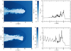 |
Fig. 1. Top panels: (left) longitudinal cut of the density distribution in the (y, z) plane for the HD case B of paper I after 200 time units, t = 1.5 × 10⁷ yrs, and (right) maximum pressure as a function of y. Bottom panels: same as in top panel but for case D of the present paper. |
These “mini” radio sources show, in both cases, a FR II morphology with terminal shock at the heads od the jets; we highlight the maximum pressure behaviors and the well-defined cocoon. In the magnetic case the nonlinear evolution of nonaxisymmetric MHD modes begins to bend the jet, and this bending will amplify at larger distances leading to the jet breaking and the onset of warm spots. Furthermore, in the MHD case the inlet pressure is already larger than in the HD case in order to maintain radial equilibrium balance. This pressure is then further increased in the locations of magnetic pinching.
3.2. The effects of magnetization on the jet propagation
We begin our analysis from case A, with β = 1000, which corresponds to a nearly negligible value of the magnetic field. We have carried out the simulation on the same domain extension and with the same numerical resolution as in the reference case. We would then expect similar results for the two simulations, but comparing in Fig. 2 the HD top-left panel with the MHD bottom-left panel we note that while in the HD case the jet begins to spread out after it has traveled a very short distance in the ambient medium, in case A it maintains its collimation up to about 6 kpc before showing a turbulent behavior. This can be explained by looking at Fig. 3 (top panel), where we show a cut of the plasma-β distribution. The value of β at the base of the jet decreases down to ≈5−10: this implies a relevant, mainly azimuthal, contribution of the magnetic field to the jet collimation in those regions. The increase of the field is the result of the compression by backflow of the jet’s head in the early stages of the propagation. The results of case B are similar to those of case A, but with the difference that the same morphology of case A is reached at about 15−18 kpc instead of 12 kpc.
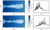 |
Fig. 2. Top panels: results for the HD case B of Paper I (M = 4, η = 10−2, ℒkin = 1.1 × 1042) at t = 640 time units, 4.9 × 10⁷ yr). Left panel: cut in the (y, z) plane of the logarithmic density distribution in units of jet density. The spatial units are in jet radii (100 pc) and the image extends over 12 kpc in the jet direction and over 6.4 kpc in the transverse direction. Right panel: maximum particle pressure as a function of y. The particle pressure is plotted in units of the ambient value (instead of the computational units |

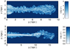 |
Fig. 3. Distribution of the plasma-β for cases A (top) and D (bottom). |
Simulations with smaller initial values (β = 10−3, cases C and D, respectively) show that the effects of magnetization begin to be important on the jet evolution. Stronger magnetization still has the same effect on the initial collimation due to the enhanced decrease in β, whose minimum is now down to 0.5 for case D (see Fig. 3, bottom panel). Below 10 kpc a signature of axially symmetric pinching modes is also evident.
Moreover, the azimuthal field induces nonaxially symmetric modes, as can be seen in both cases C (Fig. 4) and D (Fig. 5), that cause disruption of the jet. The jet then suddenly releases most of its power at about 10 kpc forming one or more warm spots, as revealed in the maximum pressure plots. With respect to the classical hot spots seen in the powerful FR II radio galaxies, the warm spots do not represent the jet termination point; beyond the warm spots the flow continues towards larger radii, instead of forming a powerful backflow. In Fig. 5 we show density cuts and maximum pressure at two different times (3.9 × 10⁷ yrs, top panels, and 5.4 × 10⁷ yrs, bottom panels) for case D: the position, relative intensities, and structure of the warm spots are not stationary in time, but they vary and wander between distances if ∼10 and ∼15 kpc from the origin of the jet. For case D we also show the 3D tracer distribution in Fig. 6 to show how the morphology gets distorted by the effect of nonaxially symmetric modes.
 |
Fig. 4. Left panel: cut of the logarithmic density distribution for case C in the (y, z) plane; right panel: maximum particle pressure as a function of y at the time t = 1100 time units, 8.4 × 10⁷ yrs. |
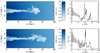 |
Fig. 5. As in Fig. 4, but for case D at t = 500 time units, 3.9 × 10⁷ yrs (top panels), and t = 700 time units, 5.4 × 10⁷ yrs (bottom panels). |
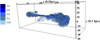 |
Fig. 6. Three-dimensional iso-contours of the tracer distribution for case D, β = 3, at t = 700 time units, 5.4 × 10⁷ yrs. The size of the computational box is 8 × 20 × 8 kpc. The x axis scales like the z one. |
Similarly to the HD simulations, in the MHD cases the advance velocity of the head of the jet, νhead, decreases with time. Figure 7 shows the results obtained for case D: after ∼300 time units νhead departs from the value based on 1D momentum conservation and this occurs at the location of the warm spots.
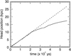 |
Fig. 7. Position of the head of the jet as a function of time for case D (solid line) compared to the theoretical value based on 1D momentum-conservation arguments (Massaglia et al. 1996). |
3.3. Distortion of the jet by a transverse wind
In Fig. 8 we see how the longitudinal velocity of the jet drops at about 10 kpc from 10 000 km s−1 to much smaller values: while there is still some flow at high velocities, most of the jet material travels at 100−1000 km s−1. Therefore, one expects that the ram pressure exerted by even moderate ICM flow velocities, with a component transverse to the jets, may be able to bend them. The resulting morphology is likely to be reminiscent of wide-angle-tail (WAT) radio galaxies (see also Soker et al. 1988 for the narrow angle tail case).
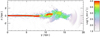 |
Fig. 8. Cut of the logarithm of the longitudinal velocity distribution for case D in the (y, z) plane. We only show the positive velocities. |
We show now the results obtained by modeling the relative motion of the galaxy in the ICM by a transverse wind with constant speed νx (Case E of Table 1). We assume that the intergalactic medium (IGM) acts as a screen to the ram pressure force exerted by the ICM wind. For the transverse ICM wind velocity we adopted the form:
 (11)
(11)
where ν∞ is the velocity of the galaxy relative to the ICM  , and α = 2. We have set ν∞ = 0.05 (case E), which in physical units corresponds to ∼100 km s−1 (see Smolčić et al. 2007), consistent with the typical velocity dispersions of galaxies in groups or poor clusters (Wilman et al. 2005).
In Fig. 9 we show the iso-contours of the tracer distribution for case E at t = 630 time units, t = 4.8 × 10⁷ yrs. We note the expected bending of the jets at a distance of about 8−9 kpc from the origin, i.e., where they disrupt. In Fig. 10 we compare the radio image of a WAT source (namely, 3C 465) with a synthetic brightness distribution ℐ(x, y) map for case E. This is obtained by integrating along the line-of-sight the 3D distribution of emissivity ϵ(x, y, z), assumed to be proportional to P(x, y, z)B2(x, y, z):
 (12)
(12)
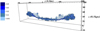 |
Fig. 9. Three-dimensional iso-contours of the tracer distribution for the WAT case E, β = 3, at t = 630 time units, 4.8 × 10⁷ yrs. The size of the computational box is 12.4 × 20 × 8 kpc. The x axis scales as in Fig. 6. |
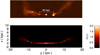 |
Fig. 10. Top panel: radio image at 4.6 GHz of 3C 465, obtained from the NRAO VLA Archive Survey Images Page (and rotated counterclockwise by 145°) showing the typical morphology of WATs. The resolution is 4″ and the FOV is 2′ × 7′, corresponding to 70 × 250 kpc. Bottom panel: cut in the (y, z) plane of the (smoothed) brightness distribution in arbitrary units at t = 630 time units for case E. |
We note the remarkable similarity of these two images but also the rather different linear scales. In the synthetic map we note the presence of a warm spot at ∼8−9 kpc, which can be clearly seen in the plot of the maximum brightness in Fig. 11.
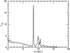 |
Fig. 11. Maximum brightness as a function of y at the time t = 630 time units for case E. |
4. Summary and conclusions
In the present paper we focused our attention on the effects of the magnetization of low-power jets. The main outcomes of this investigation can be summarized as follows:
Large values of plasma-β (∼100−1000) have the main effect of providing an additional initial collimation to the jet. In the early stages of the propagation the effective β decreases to β ∼ 5−10 due to the compression by the backflow. Since the magnetic field is mainly azimuthal the jet collimation is favored. The later evolution is similar to the HD case leading to typical FR I morphologies.
Smaller values of the plasma parameter (β ∼ 3−10) have the same effect on the initial collimation due to an even stronger decrease in the value of β. At later stages, strong nonaxially symmetric unstable modes develop leading to the sudden jet disruption at a distance of ∼10−15 kpc. Here, the jet releases most of its power, forming regions of strong emission (“warm spots”) as revealed by the maximum pressure plots. From there on, the collimation is lost and the fluid advances at subsonic speed forming diffuse plumes. This is what distinguishes these flows from those of the FR II radio galaxies, where the hot spots are located at the termination point of the jet. The warm spots are highly dynamic structures, rapidly changing with time, but always located within a small range of distances.
The abrupt velocity drop of the flow can lead, in the presence of a transverse flow (such as that due to the motion of the host galaxy), to a bending of the jet beyond the warm spots. This produces a WAT-like morphology.
The analysis of the properties of these low-power jets indicates that in both the HD and MHD cases the radio galaxies in their initial phases present the peak of maximum pressure at the head of the jet, a feature typical of FR IIs, at distances reaching about 6−8 kpc. However, radio sources with an FR I morphology and sizes in the range of only a few kiloparsecs are often observed (Balmaverde & Capetti 2006). We showed that the presence of magnetic field in these phases actually increases the jet collimation with respect to the HD case. Therefore the small FR Is are likely to be associated with jets of even lower kinetic power than those examined here (ℒkin ∼ 1042 erg s−1), in which the effects of turbulent onset destroy the jet collimation on these small scales.
The MHD simulations produce morphology, with a rapid transition from a collimated jet terminating into warm spots, to diffuse plumes reminiscent of WAT radio galaxies. Observations of WATs indicate that the separation between the two warm spots spans a large range of values, from RWS ∼ 30 to ∼240 kpc (e.g., O’Donoghue et al. 1993). In our simulations they are located at RWS ∼ 10−15 kpc and are quasi stationary, that is, their distance from the nucleus does not steadily increase with time. The largest values of RWS appear difficult to be reconciled with the simulations presented here. Most likely, larger WATs can be produced by increasing the jet power. Our simulations are performed with a rather low jet power, ℒkin = 1.1 × 1042 erg s−1. In Paper I we estimated that the transition between the two Fanaroff-Riley classes occurs at a jet power about one order of magnitude higher, while the radio power of WATs straddles the separation between FR I and FR II (Owen & Rudnick 1976). Furthermore, the jets in WATs are often highly asymmetric at a distance of several kiloparsecs from the nucleus (O’Donoghue et al. 1993), an indication of relativistic motions.
Another characteristic feature of WATs is that the diffuse plumes are bent with respect to the initial jet direction. Although the actual mechanism for bending the WAT tails remains unknown and under debate (e.g., Sakelliou & Merrifield 2000) we showed that a relative velocity of about 100 km s−1 is sufficient to bend the flow after the warm spots because the flow velocity drops suddenly.
In this paper we focused on only one parameter set, with fixed values of the Mach number and jet power, and only varied the β parameter. A more detailed investigation of the parameter space is certainly required. In particular, as noted above, WATs are likely sources associated with relativistic jets of higher power with respect to those studied in these simulations.
In this respect, it is worth noting that the high β value (and the HD case) seems to indicate that an FR I morphology is obtained with a low value of the magnetic field strength. However, this is not necessarily the case because β is the ratio between the thermal and magnetic pressure. At fixed B, one can obtain a high value of β by increasing the internal pressure of the jet. This results in a decrease of the Mach number (because M ∝ P−1) and therefore FR Is might have larger β as a consequence of a lower Mach number with respect to WATs. This is in line with the idea that the low Mach number flows are more prone to turbulence.
In Paper I and in the present paper we have used numerical simulations to analyze the dynamics of low-power jets as they propagate within the ISM at first, and then emerge into the ICM. On the bases of the tracer and density distributions and on the pressure behavior we have inferred the appearance of these objects in radio observations. A more realistic approach, however, would be to follow, alongside the jet dynamics, the evolution of the population of relativistic electrons from which the nonthermal radiation originates. Some steps in this direction have been performed by Fromm et al. (2016) and Turner et al. (2018) and a more refined treatment has recently been proposed by Vaidya et al. (2018) as a new particle module implemented in PLUTO. Further simulations of the low-power jets considered in this paper, using this module and producing more realistic synthetic radio brightness and polarization maps, will be the subject of a forthcoming paper.
We note that in Paper I the derived jet velocities, in physical units, are overestimated by about a factor of two. The values of all other parameter are unaffected.
Acknowledgments
We acknowledge support by ISCRA and by the accordo quadro INAF-CINECA 2017 for the availability of high-performance computing resources. We acknowledge also support from PRIN MIUR 2015 (grant number 2015L5EE2Y).
References
- Balmaverde, B., & Capetti, A. 2006, A&A, 447, 97 [NASA ADS] [CrossRef] [EDP Sciences] [Google Scholar]
- Bicknell, G. V. 1984, ApJ, 286, 68 [NASA ADS] [CrossRef] [Google Scholar]
- Bicknell, G. V. 1986, ApJ, 300, 591 [NASA ADS] [CrossRef] [Google Scholar]
- De Young, D. S. 1993, ApJ, 405, L13 [NASA ADS] [CrossRef] [Google Scholar]
- Ehlert, C., Weinberger, R., Pfrommer, C., Pakmor, R., & Springel, V. 2018, MNRAS, 481, 2878 [NASA ADS] [CrossRef] [Google Scholar]
- Fanaroff, B. L., & Riley, J. M. 1974, MNRAS, 167, 31P [Google Scholar]
- Fromm, C. M., Perucho, M., Mimica, P., & Ros, E. 2016, A&A, 588, A101 [NASA ADS] [CrossRef] [EDP Sciences] [Google Scholar]
- Gopal-Krishna, , & Wiita, P. J. 2000, A&A, 363, 507 [NASA ADS] [Google Scholar]
- King, I. R. 1972, ApJ, 174, L123 [NASA ADS] [CrossRef] [Google Scholar]
- Komissarov, S. S. 1990a, Ap&SS, 165, 313 [NASA ADS] [CrossRef] [Google Scholar]
- Komissarov, S. S. 1990b, Ap&SS, 165, 325 [NASA ADS] [CrossRef] [Google Scholar]
- Li, Y., Wiita, P. J., Schuh, T., Elghossain, G., & Hu, S. 2018, ApJ, 869, 32 [NASA ADS] [CrossRef] [Google Scholar]
- Massaglia, S., Bodo, G., & Ferrari, A. 1996, A&A, 307, 997 [NASA ADS] [Google Scholar]
- Massaglia, S., Bodo, G., Rossi, P., Capetti, S., & Mignone, A. 2016, A&A, 596, A12 [NASA ADS] [CrossRef] [EDP Sciences] [Google Scholar]
- Mignone, A., Bodo, G., Massaglia, S., et al. 2007, ApJS, 170, 228 [Google Scholar]
- Mignone, A., Rossi, P., Bodo, G., Ferrari, A., & Massaglia, S. 2010, MNRAS, 402, 7 [NASA ADS] [CrossRef] [Google Scholar]
- Mignone, A., Zanni, C., Tzeferacos, P., et al. 2012, ApJS, 198, 7 [Google Scholar]
- O’Donoghue, A. A., Eilek, J. A., & Owen, F. N. 1993, ApJ, 408, 428 [NASA ADS] [CrossRef] [Google Scholar]
- Owen, F. N., & Rudnick, L. 1976, ApJ, 205, L1 [NASA ADS] [CrossRef] [Google Scholar]
- Rossi, P., Bodo, G., Capetti, S., & Massaglia, S. 2017, A&A, 606, A57 [NASA ADS] [CrossRef] [EDP Sciences] [Google Scholar]
- Rudnick, L., & Owen, F. N. 1977, AJ, 82, 1 [NASA ADS] [CrossRef] [Google Scholar]
- Sakelliou, I., & Merrifield, M. R. 2000, MNRAS, 311, 649 [NASA ADS] [CrossRef] [Google Scholar]
- Smolčić, V., Schinnerer, E., Finoguenov, A., et al. 2007, ApJS, 172, 295 [NASA ADS] [CrossRef] [Google Scholar]
- Soker, N., O’Dea, C. P., & Sarazin, C. L. 1988, ApJ, 327, 627 [NASA ADS] [CrossRef] [Google Scholar]
- Turner, R. J., Rogers, J. G., Shabala, S. S., & Krause, M. G. H. 2018, MNRAS, 473, 4179 [NASA ADS] [CrossRef] [Google Scholar]
- Vaidya, B., Mignone, A., Bodo, G., Rossi, P., & Massaglia, S. 2018, ApJ, 865, 144 [NASA ADS] [CrossRef] [Google Scholar]
- Weinberger, R., Ehlert, C., Pfrommer, C., Pakmor, R., & Springel, V. 2017, MNRAS, 470, 4530 [NASA ADS] [CrossRef] [Google Scholar]
- Wilman, D. J., Balogh, M. L., Mulchaey, J. S., et al. 2005, MNRAS, 358, 71 [NASA ADS] [CrossRef] [Google Scholar]
All Tables
All Figures
|
Fig. 1. Top panels: (left) longitudinal cut of the density distribution in the (y, z) plane for the HD case B of paper I after 200 time units, t = 1.5 × 10⁷ yrs, and (right) maximum pressure as a function of y. Bottom panels: same as in top panel but for case D of the present paper. |
| In the text | |
|
Fig. 2. Top panels: results for the HD case B of Paper I (M = 4, η = 10−2, ℒkin = 1.1 × 1042) at t = 640 time units, 4.9 × 10⁷ yr). Left panel: cut in the (y, z) plane of the logarithmic density distribution in units of jet density. The spatial units are in jet radii (100 pc) and the image extends over 12 kpc in the jet direction and over 6.4 kpc in the transverse direction. Right panel: maximum particle pressure as a function of y. The particle pressure is plotted in units of the ambient value (instead of the computational units |
| In the text | |
|
Fig. 3. Distribution of the plasma-β for cases A (top) and D (bottom). |
| In the text | |
|
Fig. 4. Left panel: cut of the logarithmic density distribution for case C in the (y, z) plane; right panel: maximum particle pressure as a function of y at the time t = 1100 time units, 8.4 × 10⁷ yrs. |
| In the text | |
|
Fig. 5. As in Fig. 4, but for case D at t = 500 time units, 3.9 × 10⁷ yrs (top panels), and t = 700 time units, 5.4 × 10⁷ yrs (bottom panels). |
| In the text | |
|
Fig. 6. Three-dimensional iso-contours of the tracer distribution for case D, β = 3, at t = 700 time units, 5.4 × 10⁷ yrs. The size of the computational box is 8 × 20 × 8 kpc. The x axis scales like the z one. |
| In the text | |
|
Fig. 7. Position of the head of the jet as a function of time for case D (solid line) compared to the theoretical value based on 1D momentum-conservation arguments (Massaglia et al. 1996). |
| In the text | |
|
Fig. 8. Cut of the logarithm of the longitudinal velocity distribution for case D in the (y, z) plane. We only show the positive velocities. |
| In the text | |
|
Fig. 9. Three-dimensional iso-contours of the tracer distribution for the WAT case E, β = 3, at t = 630 time units, 4.8 × 10⁷ yrs. The size of the computational box is 12.4 × 20 × 8 kpc. The x axis scales as in Fig. 6. |
| In the text | |
|
Fig. 10. Top panel: radio image at 4.6 GHz of 3C 465, obtained from the NRAO VLA Archive Survey Images Page (and rotated counterclockwise by 145°) showing the typical morphology of WATs. The resolution is 4″ and the FOV is 2′ × 7′, corresponding to 70 × 250 kpc. Bottom panel: cut in the (y, z) plane of the (smoothed) brightness distribution in arbitrary units at t = 630 time units for case E. |
| In the text | |
|
Fig. 11. Maximum brightness as a function of y at the time t = 630 time units for case E. |
| In the text | |
Current usage metrics show cumulative count of Article Views (full-text article views including HTML views, PDF and ePub downloads, according to the available data) and Abstracts Views on Vision4Press platform.
Data correspond to usage on the plateform after 2015. The current usage metrics is available 48-96 hours after online publication and is updated daily on week days.
Initial download of the metrics may take a while.