| Issue |
A&A
Volume 621, January 2019
|
|
|---|---|---|
| Article Number | A142 | |
| Number of page(s) | 12 | |
| Section | Astrophysical processes | |
| DOI | https://doi.org/10.1051/0004-6361/201834393 | |
| Published online | 22 January 2019 | |
Structure of a collisionless pair jet in a magnetized electron–proton plasma: flow-aligned magnetic field⋆
1
Department of Science and Technology (ITN), Linköping University, 60174 Norrköping, Sweden
e-mail: Mark.E.Dieckmann@liu.se
2
École Normale Supérieure, Lyon, CRAL, UMR CNRS 5574, Université de Lyon, 69622 Lyon, France
Received:
7
October
2018
Accepted:
13
December
2018
Aims. We study the effect a guiding magnetic field has on the formation and structure of a pair jet that propagates through a collisionless electron–proton plasma at rest.
Methods. We model with a particle-in-cell (PIC) simulation a pair cloud with a temperature of 400 keV and a mean speed of 0.9c (c - light speed). Pair particles are continuously injected at the boundary. The cloud propagates through a spatially uniform, magnetized, and cool ambient electron–proton plasma at rest. The mean velocity vector of the pair cloud is aligned with the uniform background magnetic field. The pair cloud has a lateral extent of a few ion skin depths.
Results. A jet forms in time. Its outer cocoon consists of jet-accelerated ambient plasma and is separated from the inner cocoon by an electromagnetic piston with a thickness that is comparable to the local thermal gyroradius of jet particles. The inner cocoon consists of pair plasma, which lost its directed flow energy while it swept out the background magnetic field and compressed it into the electromagnetic piston. A beam of electrons and positrons moves along the jet spine at its initial speed. Its electrons are slowed down and some positrons are accelerated as they cross the head of the jet. The latter escape upstream along the magnetic field, which yields an excess of megaelectronvolt positrons ahead of the jet. A filamentation instability between positrons and protons accelerates some of the protons, which were located behind the electromagnetic piston at the time it formed, to megaelectronvolt energies.
Conclusions. A microscopic pair jet in collisionless plasma has a structure that is similar to that predicted by a hydrodynamic model of relativistic astrophysical pair jets. It is a source of megaelectronvolt positrons. An electromagnetic piston acts as the contact discontinuity between the inner and outer cocoons. It would form on subsecond timescales in a plasma with a density that is comparable to that of the interstellar medium in the rest frame of the latter. A supercritical fast magnetosonic shock will form between the pristine ambient plasma and the jet-accelerated plasma on a timescale that exceeds our simulation time by an order of magnitude.
Key words: plasmas / methods: numerical / acceleration of particles / X-rays: binaries
Movies associated to Figs. 4 and 8 are available at https://www.aanda.org
© ESO 2019
1. Introduction
Some X-ray binaries emit jets, which are composed of electrons, positrons, and an unknown fraction of ions. Pair production by V404 Cygni during an outburst has been demonstrated by Siegert et al. (2016) and it is likely that some of these pairs enter the jet. Quantifying the baryon content of the jet is difficult because its radiation spectrum is dominated by synchrotron emissions of leptons (Fender & Gallo 2014). Diaz et al. (2013) found emissions from the jet of the X-ray binary 4U 1630-47 that are indicative of baryons but this observation could not be corroborated by Neilsen et al. (2014). Only the X-ray binary SS433 is known to have a jet with a detectable baryon component (Margon et al. 1979; Migliari et al. 2002; Waisberg et al. 2018). Its jet is significantly slower than those of other X-ray binaries. Fender & Pooley (2000) remark that the energy budget available for accelerating the jet allows for either relativistic jets of electrons and positrons or nonrelativistic baryonic jets.
Some X-ray binaries with a black hole can emit jets at least intermittently, which expand at a relativistic speed into the surrounding medium (Falcke & Biermann 1996; Mirabel & Rodriguez 1999; Fender et al. 2004; Siegert et al. 2016). The latter can be interstellar medium (ISM; Ferriere 2001) or stellar wind from the companion star of the black hole. The ISM and stellar winds are an at least partially ionized dilute gas that consists mostly of hydrogen. Radiation from the accretion disk will ionize some of the gas, particularly if it is an ultraluminous X-ray source (Poutanen et al. 2007). Waisberg et al. (2018) observed photo-ionization of material along the jet of SS433 by the radiation from its source. We can therefore expect that relativistic jets of X-ray binaries interact with an ambient plasma with a significant number density.
Interactions between the jet material and the surrounding ambient material have been studied with hydrodynamic models. A generally accepted hydrodynamic jet model (see Bromberg et al. 2011, and references therein) is that of a relativistic cylindrical jet with a planar head at its front that propagates into ambient material. This model is discussed in Fig. 1.
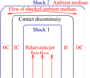 |
Fig. 1. Hydrodynamic jet model: a contact discontinuity separates the jet material from the outer cocoon, which is formed by the ambient material that was expelled by the jet. The outer cocoon is separated by the shock 2 from the ambient material that has not yet been affected by the jet. Shock 2 at the head of the jet heats the ambient material that crosses the shock and allows it to expand laterally. The shocked ambient plasma flows around the contact discontinuity and into the outer cocoon (OC). The energy required to displace the ambient material is provided by the jet material, which flows towards the contact discontinuity at a relativistic speed. It cannot cross this discontinuity; it is slowed down and heated up as it approaches it. Shock 1 forms, which separates the fast-flowing jet material from the shocked jet material close to the contact discontinuity also known as the inner cocoon (IC). The thermal pressure of the inner cocoon pushes the discontinuity outwards. |
Hydrodynamic models assume that binary collisions between particles occur fast enough to establish a thermal equilibrium of the material at any point on the relevant spatio-temporal scales. We can assign in this case unique bulk parameters such as mean speed, temperature, and density to each point in the interacting material. Shocks and discontinuities enable rapid changes of these bulk parameters.
Several X-ray binaries are close enough for us to resolve their jets in space and time. Their flow speed and temperature can therefore be determined fairly accurately from experimental observations. Hydrodynamic simulations allow us to estimate the ratio between the mass density of the jet material and that of the ambient material. Massaglia et al. (1996) performed a parametric study, in which they varied the flow speed and density ratio of the jet. They compared the structure of the jets in their simulations to observed ones and they determined parameters for which both agree reasonably well. Massaglia et al. (1996) and Dal Pino (2005) suggested that the mass density of the jet is a few per cent of that of the ambient material.
Hydrodynamic models efficiently resolve the macroscopic structure of jets, which is determined by global parameters such as the energy available to the jet and the resistance the ambient material offers to its expansion. The same is not always true for the microscopic structures. Hydrodynamic shocks between the ambient material and the outer cocoon and between the jet material and the inner cocoon and the contact discontinuity between both cocoons can only form in a collisional medium.
Jean et al. (2009) estimate that a positron with an energy of 1 MeV can propagate 30 kpc before it is decelerated by a gas with the number density 1 cm−3 to a speed at which it can recombine. Positrons with an energy that is comparable to those of the leptons carried by a mildly relativistic pair jet are thus stopped on a length scale that by far exceeds the size of the jet of an X-ray binary. Particle collisions may therefore not always be sufficiently frequent to sustain hydrodynamic shocks and contact discontinuities, which involve particles of the jet and the ambient medium in the relativistic jets of X-ray binaries.
Structures in a plasma, in which effects due to binary collisions are negligible compared to those that involve the interplay of the plasma current with the electromagnetic field, can have similar properties to hydrodynamic shocks and contact discontinuities. These structures can form on timescales that are orders of magnitude smaller than those of collisions. Such processes can be studied with particle-in-cell (PIC) codes. Their computational cost implies that we can only resolve jets that are microscopically small compared to that of an X-ray binary.
Here we study with a PIC simulation how a pair cloud interacts with a magnetized ambient plasma. The magnetic field is aligned with the direction of flow of the cloud. The pair cloud swipes out the magnetic field in its way and compresses it into an electromagnetic piston that separates the ambient from the pair plasma. The separation is almost perfect at the sides of the pair cloud. Ambient protons are accelerated away from the jet by this electromagnetic piston and they reach a few percent of the speed of light, c. The reflected protons form the outer cocoon. A magnetized collisionless shock (Shimada & Hoshino 2000; Chapman et al. 2005; Caprioli & Spitkovsky 2014; Lembege & Yang 2018) will eventually form and separate the outer cocoon from the surrounding ambient plasma. The energy loss suffered by jet particles that interact with the electromagnetic piston slows them down and an inner cocoon forms. The inner cocoons on either side of the two-dimensional jet are separated by a beam of pairs that maintain their initial speed. The microscopic jet in our simulation thus has a structure that resembles that shown in Fig. 1.
Some positrons of the relativistic beam are accelerated as they cross the head of the jet while its electrons are slowed down. The head of the jet strips off the electrons of the pair beam and is thus a source of megaelectronvolt positrons, which propagate along the magnetic field into the ISM. These positrons will eventually get stopped by their interaction with the particles and magnetic field of the ISM (Jean et al. 2009; Panther 2018).
Our paper is structured as follows. Section 2 briefly discusses the kinetic equations on which collisionless plasma is based, and the numerical scheme of a PIC code. Relevant instabilities and the findings of previous studies are summarized; the section concludes with listing our initial conditions. Section 3 shows the simulation results, which are then summarized in Sect. 4 along with a discussion of our future work aimed at addressing the matter content problem of jets.
2. Collisionless plasma and previous work
Infrequent binary collisions between particles imply that there is no constraint on the velocity distribution of particles of a given species j. Velocity becomes an independent variable and the ensemble of all particles of species j is described by a phase-space density distribution fj(x, v, t). This latter describes the probability, with which we find a particle at position x with a velocity v at the time t. Each species j of a collisionless plasma can be described by such a distribution.
A particle species is in thermal equilibrium if its density is uniform in space and if its velocity distribution is a nonrelativistic Maxwellian or a relativistic Maxwell–Jüttner distribution that is isotropic in velocity space. The thermal velocity spread is defined in this case as vth, j = (kBTj/mj)(1/2) (kB, Tj, mj: Boltzmann constant, temperature, and particle mass).
Individual plasma particles are charged and their microscopic current density is proportional to their velocity. By summing up the charge- and current-density distributions of all particles of species j we obtain its charge density ρj(x, t)=qj∫fj(x, v, t) dv and the macroscopic current density Jj(x, t)=qj∫v fj(x, v, t) dv. A summation over all species yields the total charge density ρ = ∑jρj and current density J = ∑jJj. Both are coupled to the macroscopic electric E and magnetic B fields via the Maxwell equations

where ϵ0 and μ0 are the vacuum permittivity and permeability, respectively. Both field components act back on the particle i of species j via the relativistic Lorentz force
where pi = mjΓivi and  ).
).
Absent collisions between particles allow for many features not found in a collisional medium. Several beams of charged particles with different mean speeds can, for example, coexist in the same spatial interval. These beams relax via the electromagnetic fields that are driven by collisionless plasma instabilities. The filamentation instability of counterstreaming beams of charged particles (a review is provided by Bret et al. 2010) and the Weibel (1959) instability of one plasma species with a thermal anisotropy were examined with PIC simulations in order to determine if they can generate magnetic fields and shocks in electron-positron plasma (Kazimura et al. 1998; Silva et al. 2003; Hededal & Nishikawa 2005; Chang et al. 2008; Dieckmann & Bret 2018; Plotnikov et al. 2018) and in electron-ion plasma (Spitkovsky 2008).
Amato & Arons (2006) investigated pair plasma with a minor fraction of ions for the case of ultrarelativistic shocks with a strong transverse magnetic field. They found that the pairs form increasingly nonthermal distributions as the fraction of ions in the upstream medium is increased and that the heating is stronger for positrons than for electrons. However, the one-dimensional geometry of their simulation suppressed the filamentation instability, which is dominant for such high shock speeds.
The interaction of a hot expanding pair cloud with a cooler unmagnetized ambient electron-proton plasma was studied by Dieckmann et al. (2018a) in one spatial dimension. They found that the streaming electrons and positrons drive ion acoustic solitary waves. These waves eventually break and form electrostatic shocks (Malkov et al. 2016), which can accelerate protons to high energies. Dieckmann et al. (2018b) studied this expansion in two dimensions. A filamentation instability between the cloud particles and the ambient plasma resulted in the growth of magnetic fields that separated the protons and positrons in space.
All aforementioned simulations assumed that the plasma is uniform orthogonal to the plasma flow direction and shock normal. Collisions of cylindrical plasma clouds with a spatially uniform plasma have also been modeled. Nishikawa et al. (2016) examined how cylindrical clouds of electrons and positrons or electrons and ions interact with an electron-ion plasma. A three-dimensional geometry was resolved and a reduced ion mass was used to speed up the simulation. The cloud particles had a low temperature and a highly relativistic mean speed. They interacted with the ambient plasma via Weibel and mushroom instabilities (Alves et al. 2015). Nishikawa et al. (2017) investigated the effects of a helical magnetic field for a similar plasma configuration. Dieckmann et al. (2018c) considered a hot mildly relativistic pair cloud that expanded into an unmagnetized electron-proton plasma. A jet formed. Magnetic fields due to the Weibel instability separated the jet plasma from the ambient plasma and acted as a contact discontinuity in a collisionless plasma.
3. Code and initial conditions
The PIC simulation code EPOCH defines E and B on a numerical grid and updates them in time with a numerical approximation of Eqs. (1) and (2). The current density J is obtained from the plasma. Each species j is approximated by an ensemble of computational particles (CPs), which have the same charge-to-mass ratio as the species j. The electromagnetic fields are interpolated from the grid to the position of each CP and its momentum is updated with a numerical approximation of the relativistic Lorentz force. Each CP carries with it a current that is deposited on the grid using the Esirkepov (2001) scheme. The summation of the contributions to the current density of all particles of all species j yields J, which is then used to update the electromagnetic fields. EPOCH fulfills Gauss’ law and ∇ ⋅ B = 0 to round-off precision and is discussed in detail by Arber et al. (2015).
We resolve the x-y plane and all three velocity components of the CPs. The box length of the simulation along x is Lx and 0 ≤ x ≤ Lx. The values of y span the interval −Ly/2 ≤ y ≤ Ly/2. The boundary conditions are periodic along y and reflecting along x. The simulation box is filled with a spatially uniform ambient plasma, which consists of electrons and protons with identical number densities n0 and temperatures T0 = 2 keV. All plasma density distributions will be normalized to n0. Each species is represented by 14 CPs per cell. The plasma frequencies of the electrons with the mass me and protons with the mass mp = 1836me are ωpe = (n0e2/ϵ0me)1/2 and  , respectively (e: elementary charge).
Space is normalized by the proton skin depth λs = c/ωpp as x → x/λs. Our simulation grid resolves Lx = 24.6 with 14 000 cells and Ly = 12.3 with 7000 cells. The ambient plasma is permeated at the time t = 0 by a magnetic field B0 = (B0, 0, 0) with an amplitude that yields the electron gyro-frequency ωce = eB0/me = ωpe/11.3. The magnetic energy density or pressure  equals the thermal pressure PTE = n0kBT0 of the electrons (kB: Boltzmann constant). We express E and B in units of cωpeme/e and ωpeme/e.
The pair cloud, which will drive a jet into the ambient plasma in our simulation, consists of electrons and positrons with the temperature 400 keV. This value is comparable to the brightness temperature 100 keV given by Dhawan et al. (2000) for the jet of GRS 1915+105. The brightness temperature can serve as an estimate for the average particle temperature within the jet.
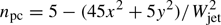
We select the mean speed 0.9c for the jet plasma, which is comparable to the speed of the superluminal jet of GRS 1915+105. A ratio of 0.005 is taken between the mass density of the pair cloud on its spine and that of the ambient plasma. This ratio is similar to the value proposed by Massaglia et al. (1996). The density distribution of our pair cloud is  if npc(x, y)≥0 and zero otherwise (see Fig. 2). The half-width of the jet is Wjet = 1.7.
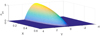 |
Fig. 2. Initial density distribution |
Each cloud species is resolved by 2 × 10⁸ CPs at the time t = 0. Additional pairs with the density distribution 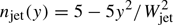 for |y|< Wjet are injected next to the boundary at x = 0. They maintain the density distribution at the cross section x = 0 of the cloud distribution in Fig. 2 while the cloud is expanding to larger x. We inject 1.6 × 10⁵ CPs at every time step. Time is normalized by
  as t → tωpp. The simulation time tsim = 34 is resolved by 62 500 steps.
The dynamics of a collisionless plasma that obeys the Maxwell–Lorentz set of equations does not change qualitatively with the value of n0 as long as we keep the density ratios of all plasma species and the ratio between the electron plasma- and gyrofrequency unchanged. Space, time, and B0 scale in this case with λs,  and ωpp. Table 1 gives the physical values of tsim, Wjet and B0 for several densities n0 of the ambient plasma.
Physical values for the simulation time tsim, the half-width of the jet Wjet, and the initial amplitude B0 of the background magnetic field for selected values of the ambient plasma density n0.
4. Simulation results
Below we discuss the global evolution of the particle and field distributions at the times t1 = 6.8, t2 = 13.6, t3 = 20.4, t4 = 27.3 and tsim. Effects due to the proton gyromotion can be neglected because ωcp/ωpp ≈ 0.002 (ωcp = ωce/1836: proton gyro-frequency). We observe the formation and early evolution of the external shock. The second subsection examines the plasma close to the external shock at the time tsim.
Electromagnetic waves emitted at x = 0 at the time t = 0 travel to the boundary at x = 24.6, are reflected by it, and return to x = 15.2 at the time tsim. Processes in the interval 0 ≤ x ≤ 14 are thus not affected by the reflecting boundary at x = 24.6 for times t ≤ tsim and we limit our investigation to this spatial window.
4.1. Global evolution
Unless stated otherwise all data were averaged over four cells along x and over four cells along y. Figures 3a,b show the density distributions of the electrons and positrons of the cloud at t = t1. Their density peaks at x = 0 in the interval |y|≤1.7 where they are injected at the left boundary.
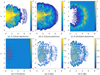 |
Fig. 3. Plasma and field distributions at t1 = 6.8. Panels a and b: distributions of the cloud electrons and positrons. The electrons and protons of the ambient plasma are shown in panels c and d, respectively. Panel e: electric field modulus |E|, and |B| is shown in panel f. The electric and magnetic amplitudes are clamped to values 0.1 and 0.2 to remove the noise. |
Both distributions extend well beyond their initial front in Fig. 2. The bulk of the cloud electrons is confined to values x ≤ 5 and |y|≤2.5 while the front of the positrons has propagated farther by a distance ≈1. The front of the pair cloud has crossed the distance ≈5 along x during the time interval t1. Its speed is thus ≈0.7c. It has crossed the distance ≈0.8 along y, giving the lateral expansion speed 0.12c.
The distance from the initial cloud border Wjet to y = 2.5 is comparable to the normalized relativistic gyro-radius rge = Γ0meV0/(eB0λs) ≈ 0.54 ( ) of a lepton moving with the speed V0. The rapid initial expansion of the pair cloud along y and across the magnetic field is caused by a gyromotion of its particles. Dilute electron and positron populations, which originated from the front of the initial cloud distribution at x ≈ 0.5, have reached x ≈ 7. Their speed is just below c.
The ambient electrons in Fig. 3c were evacuated at low values of x, |y| in the spatial region that is occupied by cloud electrons. They have been compressed in the interval, in which the front of the positrons is located. Figures 3a–c therefore demonstrate that the electrons in the cloud are slowed down by their interaction with the ambient plasma while the positrons are accelerated.
Dieckmann & Bret (2018) examined the expansion of a shock-heated pair cloud into a cooler unmagnetized pair plasma at a speed ≈V0. The shock-heated pair cloud interacted with the ambient pair plasma via the two-stream instability, which saturated by forming electrostatic phase space vortices in the electron and positron distributions. An electron phase space vortex is tied to a local excess of positive charges. Trapped electrons gyrate in the associated positive potential. A localized negative potential traps positrons. Certain combinations of the electric field and the particle distributions yield stable nonlinear structures (Schamel 1986). The symmetry between electrons and positrons and thus between their nonlinear structures resulted in both species having an equal expansion speed.
In the case we consider here the electrons of the cloud can interact with those of the ambient plasma by forming phase-space vortices. A phase-space vortex mixes them in phase space. This mixing transports the ambient electrons away from the cloud’s source in the propagation direction of the phase-space hole. Positron phase-space vortices cannot trap and accelerate protons due to their large mass difference (see the simulation by Dieckmann et al. 2018a for a detailed discussion). The population of the comoving ambient and cloud electrons is therefore denser than that of the positrons. Any excess of negative current drives a positive electric field via Ampère’s law, which decelerates the electrons and accelerates the positrons. The fastest positrons eventually outrun the slower-mixed electron population and build up a layer ahead of them that carries an excess positive current. This current drives an electric field, which accelerates and compresses the ambient electrons found in the layer with a normalized density of 2 − 4 in Fig. 3c close to the pristine ambient electrons.
Figure 4 compares the magnetic Bz component, which is driven by the filamentation instability in the considered geometry, and the modulus of the in-plane magnetic field.
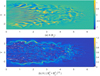 |
Fig. 4. Magnetic field distributions at t1 = 6.8. Panel a: out-of-plane magnetic field Bz, which is driven by the filamentation instability. Panel b: modulus of the in-plane magnetic field. See online movie 1 for a time-animation for 0 ≤ t ≤ tsim. |
We observe peak values of the magnetic field that exceed B0 by an order of magnitude. The in-plane magnetic field in Fig. 4b is weaker than Bz at this time except in some locations close to the boundary of the pair cloud. Supplementary movie 1 animates Fig. 4 in the time interval 0 ≤ t ≤ tsim. It shows how the Bz component driven by the filamentation instability weakens in time while the magnetic band in the in-plane magnetic field distribution strengthens in time.
The protons close to x = 0 in Fig. 3d have been compressed into thin filaments. The pair cloud and the ambient plasma interact via a filamentation instability, which is responsible for the strong magnetic field in Fig. 4a that follows the proton density filaments. The electromagnetic fields close to the cloud front in Fig. 3 have a different structure and they are a result of the aforementioned two-stream instability, which is not purely electrostatic for relativistic speeds (Bret et al. 2010).
Figure 5 shows the plasma and field distributions at the time t2. The cloud front at x ≈ 2 has expanded from y ≈ 2.6 at t = t1 to y ≈ 2.9 at t = t2, which yields a front speed of about 0.04c along y; the lateral expansion of the cloud has been slowed down by B0. Figures 3a and 5a show that the cloud electrons have expanded from x ≈ 5 at t1 until x ≈ 7 at t2, which yields the speed c/3.
 |
Fig. 5. Plasma and field distributions at t2 = 13.6. Panels a and b: distributions of the cloud electrons and positrons. The electrons and protons of the ambient plasma are shown in panels c and d, respectively. Panel e: electric field modulus |E|, and |B| is shown in panel f. The electric and magnetic amplitudes are clamped to values 0.1 and 0.2 to remove noise. |
Positrons have expanded farther in all directions and a beam with a density ∼0.5 has formed at large x and |y|≤2.
The pair cloud continued to expel ambient electrons in Fig. 5c. A thin band with a density value ≈4 in Fig. 5c marks the end of the spatial interval, which is occupied by the cloud plasma. A similar high-density band is seen in the protons for x ≤ 4 and |y|≈2.8. The high-density band is accompanied by strong electromagnetic fields in Figs. 5e,f. The latter also show strong filaments at low values of x, |y|, which follow those in the proton density distribution in Fig. 5d. The filamentation of the protons has continued and their density has decreased to almost zero in extended spatial intervals.
The cloud electrons at the time t3 are confined to a smaller spatial interval in Fig. 6a than the positrons in Fig. 6b.
 |
Fig. 6. Plasma and field distributions at t3 = 20. Panels a and b: distributions of the cloud electrons and positrons. The electrons and protons of the ambient plasma are shown in panels c and d, respectively. Panel e: electric field modulus |E|, and |B| is shown in panel f. The electric and magnetic amplitudes are clamped to values 0.1 and 0.2 to remove noise. |
Only electrons from the cloud can compensate the charge imbalance caused by the expulsion of the ambient electrons in Fig. 6c. For this reason they accumulate where the ambient electrons were expelled.
The ambient electrons and protons still show a high-density band. It was located at |y|≈2.8 at t = t2 and x ≈ 2 and at |y|≈3.1 at the same value of x in Fig. 6d and the expansion speed along y is ≈0.04c. No high-density band can be observed at the front of the cloud at x ≈ 7 at low |y|. Positrons flow out along B0 in this y-interval and their charge is compensated by an accumulation of the ambient electrons. A filamentation instability continues to develop in the interval x < 4.5 and |y|≤2 between the particles of the pair cloud and the protons and we observe the strongest proton density filaments at x ≈ 4 and |y|≤1.5. The electromagnetic fields associated with the high-density band that encloses the pair cloud are now stronger than those driven by the filamentation instability within the pair cloud.
Figure 7 shows that the high-density band and its associated electromagnetic fields mark the boundary between the cloud in Figs. 7a,b and the ambient electrons and protons in Figs. 7c,d. The protons have been completely expelled from an interval with the width ∼0.25 directly behind the high-density band. Figures 7e,f reveal a continuing weakening of the electromagnetic fields, which are associated with the filamentation instability between the pair cloud and the protons in the interval x ≤ 4 and |y|≤2 while those associated with the high-density band have maintained their strength.
 |
Fig. 7. Plasma and field distributions at t4 = 27.5. Panels a and b: distributions of the cloud electrons and positrons. The electrons and protons of the ambient plasma are shown in panels c and d, respectively. Panel e: electric field modulus |E|, and |B| is shown in panel f. The electric and magnetic amplitudes are clamped to values 0.1 and 0.2 to remove noise. |
Figure 8 shows the distributions of the plasma species and of the electromagnetic fields at the final time tsim. Figure 8 is animated in the supplementary movie 2 that covers the time interval 0 ≤ t ≤ tsim.
 |
Fig. 8. Plasma and field distributions at tsim = 34. Panels a and b: distributions of the cloud electrons and positrons. The electrons and protons of the ambient plasma are shown in panels c and d, respectively. Panel e: electric field modulus |E|, and |B| is shown in panel f. The electric and magnetic amplitudes are clamped to values 0.1 and 0.2 to remove noise. See online movie 2 for a time-animation for 0 ≤ t ≤ tsim. |
The distributions resemble qualitatively those at t = t4 and a stable state has been reached. The thickness of the interval from which the protons were evacuated has increased to about 0.5 and this is therefore an ongoing process. The front of the cloud electrons has propagated from x ≈ 9.5 at t = t4 to about x ≈ 10.5 at t = tsim at the speed 0.15c. The high-density band in the protons and ambient electrons is accompanied by a thin electromagnetic sheath in Figs. 8e,f. It does not fully enclose the pair plasma at the cloud front at x ≈ 10 and we continue to observe an outflow of positrons at large x and |y|≤2.
Density filaments, which are spatially correlated and approximately aligned with x, are present in the distributions of the protons and ambient electrons in the interval x > 10 and |y|≤1.5. We cannot observe magnetic field structures in Fig. 8f that follow these density striations. Their field amplitude is below the threshold 0.2 and small compared to the magnetic fields driven by the clumpy positron distribution in this interval.
The pair cloud is progressively separating itself from the ambient plasma close to the high-density band. A pair flow, which is separated from the ambient plasma, is a jet and hence we are observing its formation. The work that is required to expel the ambient plasma slows down the pair cloud close to the thin strong electromagnetic sheath and an inner cocoon forms. The accompanying movie shows structures in the density distribution of the pair cloud that are deflected sideways and slowed down at the thin strong electromagnetic sheath. The cloud electrons are separated from the ambient electrons at the head of the jet at x ≈ 8 and the ambient protons are deflected sideways at |y|≥2. Our collisionless jet shows some features of a hydrodynamic jet.
4.2. The electromagnetic piston and the pair flow at the head
We investigate here the high-density band in the ambient plasma and the structure of the electromagnetic fields that sustain it. We focus on a jet interval where the high-density band is propagating orthogonally to the main axis of the jet.
Figure 9 shows the spatial distributions of the in-plane electric field components Ex and Ey, those of the in-plane magnetic field components Bx and By, and of their normalized energy densities  and
and  at the time t = tsim. Lineouts of all field components are also plotted.
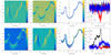 |
Fig. 9. Electromagnetic fields at the time t = tsim in full spatial resolution. Panels a and b: electric Ex and Ey components. The pressure |
Both electric field components in Figs. 9a,b and their energy density show a banded structure, which is double-peaked in some intervals. The electric field band follows the unipolar magnetic field band in Fig. 9g. The amplitude of Bx reaches more than 30 times the value B0 = 0.0884 in this band. Large amplitudes of By are observed in Fig. 9f in the intervals where Bx is weak and aligned with y in Fig. 9e; both components belong to the same band and their respective amplitudes depend on the orientation of the band. Figure 9g reveals that the magnetic energy density in the center of this magnetic band exceeds PTE by a factor ≥200 almost everywhere. The energy density rises to more than 800 PTE in some intervals with a high curvature. We observe a thickening of the magnetic band for 3.4 ≤ x ≤ 4.1.
A comparison of the lineouts at x = 3.6 in Figs. 9d and h shows that the large peak of Bx at y = −3.9 coincides with a negative Ey and that the other field components are weak at this location. We refer to this magnetic band and the electric field structure that is enclosing it as the electromagnetic piston. Figure 9h demonstrates that the amplitude of Bz, which is at least partially driven by the Weibel instability between the pair cloud and the protons behind the electromagnetic piston, is significantly lower than that of Bx at y = −3.9. The mean value of Bx over the interval −4.4 ≤ y ≤ −4.3 along x = 3.6 is comparable to B0 while the mean value in the interval −3.75 ≤ y ≤ −3.65 is about B0/25; the pair plasma has swiped out the background magnetic field and piled it up at the electromagnetic piston.
We estimated the thermal gyroradius of an electron or positron of the cloud in a field with the amplitude B0 as rge ≈ 0.54. The magnetic field reaches a peak value of more than 15B0, which decreases the local thermal gyroradius to a value that is below the thickness of the electromagnetic piston. Figure 10 depicts the effect the electromagnetic piston has on the particle populations.
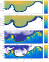 |
Fig. 10. Density distributions of the cloud electrons (a), of the positrons (b), of the ambient electrons (c), and protons (d) at the time t = tsim. The contours PB = 200 are overplotted. |
The electrons and positrons of the cloud in Figs. 10a,b are indeed confined by the electromagnetic piston. The density distributions of the cloud particles behind the electromagnetic piston are almost uniform. Some positrons penetrate deeper into the electromagnetic piston than the electrons at x ≈ 3.6 and y ≈ −3.9 and their current may be responsible for the thickening of the magnetic band in Fig. 9g.
Most ambient electrons in Fig. 10 are confined to values of y below those of the electromagnetic piston. They cannot overcome the magnetic field of the electromagnetic piston and are pushed by it to lower y. Only a few ambient electrons are found at larger y. The density of the ambient electrons exceeds 6 in intervals close to the cusps of the electromagnetic piston.
The ambient protons are also mostly confined to values of y that are lower than that of the electromagnetic piston. Even the strong magnetic field of the electromagnetic piston cannot expel the protons via Larmor rotation. Its electric field is responsible for the proton acceleration. The proton density follows that of the ambient electrons and its peak value exceeds 6 close to the cusps of the electromagnetic piston. Some protons managed to break through the electromagnetic piston at x= 3.2 and y = −3.4. The magnetic pressure of the electromagnetic piston is reduced by about 30% at this location. The value of the magnetic pressure is below that of the contour line, which results in the apparent gap (see also Fig. 9f). A dilute proton population is found at large y far behind the expanding electromagnetic piston. These protons were located behind the electromagnetic piston when it formed and hence they could not get swept out by it.
Figure 11 shows the proton velocity and density distributions along the slice x = 3.6.
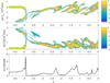 |
Fig. 11. Proton distribution along the slice x = 3.6 for y ≤ 0 at t = tsim. Panel a: phase space density distribution along the cut plane y and vy. Panel b: distribution along y and the velocity modulus |
A single population of cool protons at rest, which have retained their initial conditions, is located in the interval y ≤ −4.5. Protons are accelerated to a speed of −2.5 × 10⁷ m s−1 at the position y ≈ −3.9, which is where the electromagnetic piston is located in Fig. 9. Protons with the speed 2.5 × 10⁷ m s−1 have a kinetic energy of 4.7 MeV, which exceeds the thermal energy of the jet by an order of magnitude. Figure 11b demonstrates that the distribution of y, vy matches that of y, |v| apart from the opposite sign. Protons in the lineout x = 3.6 are thus accelerated only along y. If we assume that these protons have been reflected specularly by the electromagnetic piston then the latter is propagating at the speed vs = −1.25 × 10⁷ m s−1 or −0.04c. This speed matches the expansion speed we estimated by comparing the locations of the piston along y in Figs. 6–8. Figure 11c provides evidence that the proton density is almost zero behind the electromagnetic piston and below 0.1 for −3.9 ≤ y ≤ −3.3.
The electromagnetic piston separates the jet plasma from the ambient plasma and its role is that of the contact discontinuity in hydrodynamic jets. Eventually a collisionless shock (shock 2 in Fig. 1) must form between the pristine ambient plasma, which is located at y ≤ −4.5 in Fig. 11a, and the accelerated one in the interval −4.5 ≤ y ≤ −3.9. The nature of the shock will depend on how the collision speed between both ambient plasma populations compares to the characteristic plasma speeds.
The ion acoustic speed in the ambient plasma is cs = (kB(γeTe + γiTi)/mp)1/2, where the electron and proton temperatures Te = Tp = T0. Electrons have 3 degrees of freedom (γe = 5/3) in a collisionless plasma and protons 1 (γp = 3) and cs ≈ 106 m s−1. The electromagnetic piston has the speed ≈13cs. Electrostatic shocks, which are mediated by the ambipolar electric field across a density gradient, cannot form at this high collision speed (Forslund & Freidberg 1971; Dieckmann et al. 2013) and the shock must be magnetized.
The electromagnetic piston moves orthogonally across the initial magnetic field in Fig. 11 and a shock will involve the fast magnetosonic mode. The Alfvén speed vA = B0/(μ0n0mp)≈6.2 × 105 m s−1 gives the fast magnetosonic speed  m s−1. The electromagnetic piston moves at the speed 11 vfms and the shock will be a supercritical fast magnetosonic shock (Marshall 1955). Such shocks form on timescales that exceed an ion gyroperiod in the magnetic field B0 (Shimada & Hoshino 2000; Chapman et al. 2005; Caprioli & Spitkovsky 2014; Lembege & Yang 2018). The formation time of such a shock exceeds tsim by at least an order of magnitude. Therefore, we cannot observe the formation of an external shock between the pristine ambient plasma and the accelerated ambient plasma, which constitutes the outer cocoon.
Figures 11a,b show energetic protons in the interval y > −3.9. The modulus of their peak speed is below |vs| and they are outrun by the electromagnetic piston. The distributions along vy and along |V| hardly differ apart from the wrap-around at vy = 0 and they have thus also been accelerated mainly along y. Their peak speed of 107 m s−1 is comparable to that of the protons in the simulation by Dieckmann et al. (2018b) and they have thus been accelerated by the filamentation instability that formed initially between the pair cloud and the ambient plasma.
We analyze the phase-space density distributions of the positrons and electrons where we do not distinguish between ambient and jet electrons. We consider the phase-space density as a function of x, y and the energy Ekin = p2/2me, where p is the relativistic particle momentum. Phase-space densities are integrated over 20 cells along x and along y and are normalized to the peak density of the electrons. We show three isosurfaces that correspond to contours of the phase-space density. The iso-surface with the density contour 30−1 in Fig. 12 encloses the bulk of the particles. The density contour 30−2 in Fig. 13 wraps around the particles with intermediate energies while the high-energy particles (density contour 30−3) are shown in Fig. 14.
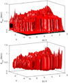 |
Fig. 12. Isosurfaces 30−1 for the phase-space density distribution fe(x, y, Ekin) of the electrons (panel a) that of the positrons (panel b) at the time tsim. The phase space densities are normalized to the peak density of the electrons. |
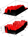 |
Fig. 13. Isosurfaces 30−2 for the electrons phase space density distribution fe(x, y, Ekin) (panel a) and that of the positrons (panel b) at the time tsim. The phase space densities are normalized to the peak density of the electrons. |
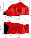 |
Fig. 14. Isosurfaces 30−3 for the electrons phase space density distribution fe(x, y, Ekin) (panel a) and that of the positrons (panel b) at the time tsim. The phase space densities are normalized to the peak density of the electrons. |
Figure 12 shows the distributions of electrons and positrons with low energy.
Both distributions resemble each other for x < 8 and for energies above 300 keV. Electrons with lower energies stem from the ambient electrons, which have no positronic counterpart in Fig. 12b. Electrons and positrons are confined at large |y|. The bulk of the pairs is limited to energies below 1 MeV, which corresponds to the typical energy expected from leptons moving in a hot jet plasma with the mean speed 0.9c.
We observe significant differences between the populations of electrons and positrons in Fig. 13.
The electron distribution within the jet reaches a uniform maximum energy of 1.5 MeV for the selected density contour and it decreases rapidly at the jet boundary. We find more positrons with a higher energy close to the electromagnetic piston than inside the jet.
Figure 14 shows that the electrons and positrons reach comparable peak energies far from the electromagnetic piston and the head of the jet at x ≈ 12. More energetic positrons are observed close to the electromagnetic piston at y ≈ −3.5 and x < 10.
Figure 14 also reveals an outflow of energetic positrons along the jet spine y ≥ −3, which has no counterpart in the electron distribution. The jet is thus a source of multi-MeV positrons that propagate along its expansion direction.
Figures 10, 13, and 14 hint at how the electromagnetic piston is sustained; it forms a barrier for the ambient electrons (see Fig. 10c). As the electromagnetic piston swipes out the ambient electrons, an electric field must grow that drags the protons with them (see Fig. 10d) to maintain the quasi-neutrality of the plasma. The magnetic field of the electromagnetic piston can only be supported by the currents of relativistically fast particles. These currents must flow orthogonally to the simulation box in order to support the in-plane magnetic field of the piston. Figures 13 and 14 reveal that we find more positrons than electrons with energies above 2 MeV close to the piston. The gyroradius 0.062 of an electron or positron with 2 MeV in a field with the magnetic amplitude 1.7 in Fig. 9h is comparable to the thickness of the electromagnetic piston. These energetic particles can therefore penetrate deep into this structure, which is also demonstrated by Figs. 10a,b. Having more energetic positrons than electrons implies that the electromagnetic piston is immersed in a net positronic current contribution. Figures 5–8 demonstrate that the electromagnetic piston is stable on timescales tsim. The interplay of the electromagnetic piston with the energetic cloud particles around it yields a stable magnetic field configuration in the same way that magnetic boundaries in electron-ion plasmas can be sustained by the electron current (Grad 1961).
Figure 15 shows the momentum distributions of the electrons and positrons along x averaged over the interval −0.35 ≤ y ≤ 0.
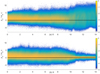 |
Fig. 15. 10-logarithmic phase space density along x and px of the positrons (panel a) and electrons (panel b) in the interval −0.35 ≤ y ≤ 0. Both are normalized to the peak density in panel b. Horizontal lines px = 0 are overplotted. |
Both distributions demonstrate that most electrons and positrons maintain their initial momentum in the interval x ≤ 8. A high-speed flow channel thus exists close to the spine of the collisionless jet. The momentum spread of the electrons decreases in the head of the jet with 8 ≤ x ≤ 11 and that of the positrons increases. We find more electrons with px/mec ≤ −3 in the interval x ≤ 7 than positrons. Jet electrons are reflected at the head and return to the injection point while positrons are accelerated at the head and stream out to larger x. This loss of positrons reduces the number of returning positrons in the interval x ≤ 7. Some ambient electrons reach mildly relativistic speeds in the interval x > 11. They have been heated by the filamentation instability between the positrons and the ambient plasma. This filamentation instability is also heating up the positrons. Positrons in the interval x > 11 are scattered by the electromagnetic fields to values px < 0, which increases their thermal spread.
5. Discussion
We have used a PIC simulation to examine the interaction between a hot and fast cloud of electrons and positrons with a cool ambient magnetized plasma composed of electrons and protons. The magnetic field was aligned with the mean flow direction of the pair cloud. The magnetic field amplitude was selected such that the gyroradius of the pair cloud’s particles remained small compared to the distance between the pair cloud and the boundaries along y. The magnetic pressure remained small compared to the thermal pressure of the pair cloud.
Initially the pair cloud expanded almost freely at its initial mildly relativistic speed. Larmor rotation slowed down the lateral expansion of the pair cloud while a filamentation instability developed between the pair cloud and the ambient plasma. Its magnetic field was significantly stronger than the background magnetic field and this instability was thus similar to that in the unmagnetized plasma observed by Dieckmann et al. (2018b). This filamentation instability heated the protons to megaelectronvolt temperatures. The expanding pair cloud swiped out the background magnetic field and piled it up into an electromagnetic piston. Its magnetic field vector was oriented in the simulation plane and this structure was therefore not generated by the filamentation instability. Filamentation instabilities separate current filaments in the simulation plane and they yield magnetic fields that point orthogonally to the simulation plane.
The electromagnetic piston was strong enough to separate the pair cloud from the ambient plasma and it thus acted as a collisionless counterpart of a hydrodynamic contact discontinuity. It separated the pair cloud, with its high thermal pressure, from the ambient plasma that has a much lower thermal pressure and magnetic pressure. Consequently the electromagnetic piston propagated into the ambient plasma. It pushed out the ambient electrons and an electric field grew that dragged the protons with it. A progressive separation of the cloud plasma from the ambient plasma is evidence of a forming collisionless jet.
The propagation speed of the electromagnetic piston amounted to 0.04c in the direction that was orthogonal to the mean flow direction of the pair cloud. This propagation speed far exceeded the thermal speed of the ambient protons and we observed a fast beam of protons that were reflected by the electromagnetic piston. The speed of this beam amounted to 13 times the ion acoustic speed cs in the ambient plasma. Electrostatic shocks cannot form at such a high speed (Forslund & Freidberg 1971). The beam speed was 11 times the fast magnetosonic speed vfms in the ambient plasma. Only supercritical magnetized shocks can form at such speeds. Their formation time exceeds an inverse ion gyrofrequency and we stopped our simulation long before such a shock could form.
The jet front expanded at 0.15c along the magnetic field, which resulted in a shape that was elongated along the flow direction of the pair cloud. A reduction of the temperature of the pair plasma and an increase of its mean speed and of the magnetic field amplitude should result in a larger ratio between the longitudinal and lateral expansion speed of the jet.
Our simulation showed that the interplay of the electric and magnetic fields with the pair cloud resulted in a larger number of energetic positrons close to the electromagnetic piston. The positrons could penetrate deeper into the electromagnetic piston than the electrons and consequently a net current developed close to it that stabilized its magnetic field. A boundary of a collisionless jet that is formed by a spatially homogeneous strong magnetic field and is immersed in hot positrons and electrons should give rise to radio emissions.
The electrons and positrons that flowed along the spine of the pair cloud maintained their initial flow speed until they reached the head of the pair cloud. Electromagnetic processes close to the head of the jet slowed down the electrons of the pair cloud and accelerated its positrons, which resulted in an outflow of hot positrons along the jet axis with energies of up to 5 MeV. Some of these megaelectronvolt positrons will flow along the magnetic field and escape into the ambient plasma far from the jet. Such positrons could contribute to the galactic positron population (Panther 2018).
Previous simulations related to pair jets in unmagnetized plasmas (Nishikawa et al. 2016; Dieckmann et al. 2018c) showed that magnetic fields grow in response to the filamentation- and mushroom instabilities (Alves et al. 2015). The magnetic field of the filamentation instability could become strong enough to act as a contact discontinuity in the simulation by Dieckmann et al. (2018c). The latter simulation stabilized the jet with the help of a rigid spine. Here we have shown that a jet can also be stabilized by a guiding field with a thermal pressure that is low compared to the thermal pressure of the jet. The compressed background magnetic field replaces, in this case, that of the filamentation instability as the one that acts as a contact discontinuity.
Here we drove the jet with a pair cloud but the jet was not purely leptonic. We launched the jet in an electron-proton plasma and some protons were behind the electromagnetic piston when it formed. The electromagnetic piston was also not impenetrable to the ambient protons. Some overcame it at locations where the magnetic pressure of the electromagnetic piston was reduced and entered the inner cocoon. Protons were accelerated on short timescales and by the end of the simulation the jet had a baryon component with a thermal energy of the order of 1 MeV. The observed rapid proton acceleration was tied to the large relative speed between the protons and the pair cloud. This has consequences even for astrophysical jets. Waisberg et al. (2018) reported the observation of photo-ionization along the jet SS433. Neutrals will not interact with the electromagnetic piston and they can enter the inner jet. A filamentation instability sets in once these neutrals are ionized in significant numbers and they will rapidly be accelerated to megaelectronvolt energies and possibly beyond.
Future studies will examine how the jet, the electromagnetic piston, and the ambient plasma react to an ion beam that is propagating with the pair cloud. Fender & Pooley (2000) suggest that it is unlikely that a relativistic jet is composed solely of electrons and ions. It is however plausible that the jet carries with it a significant fraction of relativistic ions. The energy carried by a relativistic ion population implies that energetic processes other than the ones observed here may develop.
Movies
Movie of Fig. 4 Access here
Movie of Fig. 8 Access here
Acknowledgments
M. E. D. acknowledges financial support by a visiting fellowship from the Ecole Nationale Supérieure de Lyon, Université de Lyon. DF and RW acknowledge support from the French National Program of High Energy (PNHE). Simulations were performed with the EPOCH code financed by the grant EP/P02212X/1 on resources provided by the French supercomputing facilities GENCI through the grant A0030406960.
References
- Alves, E. P., Grismayer, T., Fonseca, R. A., & Silva, L. O. 2015, Phys. Rev. E, 92, 021101 [NASA ADS] [CrossRef] [Google Scholar]
- Amato, E., & Arons, J. 2006, AJ, 653, 325 [Google Scholar]
- Arber, T. D., Bennett, K., Brady, C. S., et al. 2015, Plasma Phys. Controll. Fusion, 57, 113001 [Google Scholar]
- Bret, A., Gremillet, L., & Dieckmann, M. E. 2010, Phys. Plasmas, 17, 120501 [NASA ADS] [CrossRef] [Google Scholar]
- Bromberg, O., Nakar, E., Piran, T., et al. 2011, AJ, 740, 100 [Google Scholar]
- Caprioli, D., & Spitkovsky, A. 2014, AJ, 783, 91 [Google Scholar]
- Chang, P., Spitkovsky, A., & Arons, J. 2008, AJ, 674, 378 [NASA ADS] [CrossRef] [Google Scholar]
- Chapman, S. C., Lee, R. E., Dendy, R. O. 2005, Space Sci. Rev., 121, 5 [NASA ADS] [CrossRef] [Google Scholar]
- Dal Pino, E. M. D. 2005, Adv. Space Res., 35, 908 [NASA ADS] [CrossRef] [Google Scholar]
- Dhawan, V., Mirabel, I. F., & Rodriguez, L. F. 2000, AJ, 543, 373 [NASA ADS] [CrossRef] [Google Scholar]
- Diaz, Trigo M., Miller-Jones, J. C. A., Migliari, S., Broderick, J. W., & Tzioumis, T. 2013, Nature, 504, 260 [NASA ADS] [CrossRef] [Google Scholar]
- Dieckmann, M. E., & Bret, A. 2018, MNRAS, 473, 198 [NASA ADS] [CrossRef] [Google Scholar]
- Dieckmann, M. E., Ahmed, H., Sarri, G., et al. 2013, Phys. Plasmas, 20, 042111 [NASA ADS] [CrossRef] [Google Scholar]
- Dieckmann, M. E., Alejo, A., Sarri, G., Folini, D., & Walder, R. 2018a, Phys. Plasmas, 25, 064502 [NASA ADS] [CrossRef] [Google Scholar]
- Dieckmann, M. E., Alejo, A., & Sarri, G. 2018b, Phys. Plasmas, 25, 062122 [NASA ADS] [CrossRef] [Google Scholar]
- Dieckmann, M. E., Sarri, G., Folini, D., Walder, R., & Borghesi, M. 2018c, Phys. Plasmas, 25, 112903 [CrossRef] [Google Scholar]
- Esirkepov, T. Z. 2001, Computer Phys. Comm., 135, 144 [NASA ADS] [CrossRef] [Google Scholar]
- Falcke, H., & Biermann, P. L. 1996, A&A, 308, 321 [NASA ADS] [Google Scholar]
- Fender, R., & Gallo, E. 2014, Space Sci. Rev., 183, 323 [NASA ADS] [CrossRef] [Google Scholar]
- Fender, R. P., & Pooley, G. G. 2000, MNRAS, 318, L1 [NASA ADS] [CrossRef] [Google Scholar]
- Fender, R. P., Belloni, T. M., & Gallo, E. 2004, MNRAS, 355, 1105 [NASA ADS] [CrossRef] [Google Scholar]
- Ferriere, K. M. 2001, Rev. Mod. Phys., 73, 1031 [NASA ADS] [CrossRef] [Google Scholar]
- Forslund, D. W., & Freidberg, J. P. 1971, Phys. Rev. Lett., 27, 1189 [NASA ADS] [CrossRef] [Google Scholar]
- Grad, H. 1961, Phys. Fluids, 4, 1366 [NASA ADS] [CrossRef] [Google Scholar]
- Hededal, C. B., & Nishikawa, K. I. 2005, AJ, 623, L89 [NASA ADS] [CrossRef] [Google Scholar]
- Jean, P., Gillard, W., Marcowith, A., & Ferrière, K. 2009, A&A, 508, 1099 [NASA ADS] [CrossRef] [EDP Sciences] [Google Scholar]
- Kazimura, Y., Sakai, J. I., Neubert, T., & Bulanov, S. V. 1998, AJ, 498, L183 [NASA ADS] [CrossRef] [Google Scholar]
- Lembege, B., & Yang, Z. W. 2018, AJ, 860, 84 [NASA ADS] [CrossRef] [Google Scholar]
- Malkov, M. A., Sagdeev, R. Z., Dudnikova, G. I., et al. 2016, Phys. Plasmas., 23, 043105 [NASA ADS] [CrossRef] [Google Scholar]
- Margon, B., Ford, H. C., Grandi, S. A., & Stone, R. P. S. 1979, AJ, 233, L63 [Google Scholar]
- Marshall, W. 1955, Proc. R. Soc. London A, 233, 367 [NASA ADS] [CrossRef] [Google Scholar]
- Massaglia, S., Bodo, G., & Ferrari, A. 1996, A&A, 307, 997 [NASA ADS] [Google Scholar]
- Migliari, S., Fender, R., & Mendez, M. 2002, Science, 297, 1673 [NASA ADS] [CrossRef] [PubMed] [Google Scholar]
- Mirabel, I. F., & Rodriguez, L. F. 1999, AJ, 37, 409 [Google Scholar]
- Neilsen, J., Coriat, M., Fender, R., et al. 2014, AJ, 784, L5 [CrossRef] [Google Scholar]
- Nishikawa, K. I., Frederiksen, J. T., Nordlund, A., et al. 2016, AJ, 820, 94 [CrossRef] [Google Scholar]
- Nishikawa, K. I., Mizuno, Y., Gomez, J. L., et al. 2017, Galaxies, 5, 58 [NASA ADS] [CrossRef] [Google Scholar]
- Panther, F. H. 2018, Galaxies, 6, 39 [NASA ADS] [CrossRef] [Google Scholar]
- Plotnikov, I., Grassi, A., & Grech, M. 2018, MNRAS, 477, 5238 [NASA ADS] [CrossRef] [Google Scholar]
- Poutanen, J., Lipunova, G., Fabrika, S., Butkevich, A. G., & Abolmasov, P. 2007, MNRAS, 377, 1187 [NASA ADS] [CrossRef] [Google Scholar]
- Schamel, H. 1986, Phys. Rep., 140, 161 [NASA ADS] [CrossRef] [Google Scholar]
- Shimada, N., & Hoshino, M. 2000, AJ, 543, L67 [NASA ADS] [CrossRef] [Google Scholar]
- Siegert, T., Diehl, R., Greiner, J., et al. 2016, Nature, 531, 341 [NASA ADS] [CrossRef] [Google Scholar]
- Silva, L. O., Fonseca, R. A., Tonge, J. W., et al. 2003, AJ, 596, L121 [NASA ADS] [CrossRef] [Google Scholar]
- Spitkovsky, A. 2008, AJ, 673, L39 [NASA ADS] [CrossRef] [Google Scholar]
- Waisberg, I., Dexter, J., Olivier-Petrucci, P., Dubus, G., & Perraut, K. 2018, A&A, submitted [arXiv:1811.12564] [Google Scholar]
- Weibel, E. S. 1959, Phys. Rev. Lett., 2, 83 [NASA ADS] [CrossRef] [Google Scholar]
All Tables
Physical values for the simulation time tsim, the half-width of the jet Wjet, and the initial amplitude B0 of the background magnetic field for selected values of the ambient plasma density n0.
All Figures
|
Fig. 1. Hydrodynamic jet model: a contact discontinuity separates the jet material from the outer cocoon, which is formed by the ambient material that was expelled by the jet. The outer cocoon is separated by the shock 2 from the ambient material that has not yet been affected by the jet. Shock 2 at the head of the jet heats the ambient material that crosses the shock and allows it to expand laterally. The shocked ambient plasma flows around the contact discontinuity and into the outer cocoon (OC). The energy required to displace the ambient material is provided by the jet material, which flows towards the contact discontinuity at a relativistic speed. It cannot cross this discontinuity; it is slowed down and heated up as it approaches it. Shock 1 forms, which separates the fast-flowing jet material from the shocked jet material close to the contact discontinuity also known as the inner cocoon (IC). The thermal pressure of the inner cocoon pushes the discontinuity outwards. |
| In the text | |
|
Fig. 2. Initial density distribution |
| In the text | |
|
Fig. 3. Plasma and field distributions at t1 = 6.8. Panels a and b: distributions of the cloud electrons and positrons. The electrons and protons of the ambient plasma are shown in panels c and d, respectively. Panel e: electric field modulus |E|, and |B| is shown in panel f. The electric and magnetic amplitudes are clamped to values 0.1 and 0.2 to remove the noise. |
| In the text | |
|
Fig. 4. Magnetic field distributions at t1 = 6.8. Panel a: out-of-plane magnetic field Bz, which is driven by the filamentation instability. Panel b: modulus of the in-plane magnetic field. See online movie 1 for a time-animation for 0 ≤ t ≤ tsim. |
| In the text | |
|
Fig. 5. Plasma and field distributions at t2 = 13.6. Panels a and b: distributions of the cloud electrons and positrons. The electrons and protons of the ambient plasma are shown in panels c and d, respectively. Panel e: electric field modulus |E|, and |B| is shown in panel f. The electric and magnetic amplitudes are clamped to values 0.1 and 0.2 to remove noise. |
| In the text | |
|
Fig. 6. Plasma and field distributions at t3 = 20. Panels a and b: distributions of the cloud electrons and positrons. The electrons and protons of the ambient plasma are shown in panels c and d, respectively. Panel e: electric field modulus |E|, and |B| is shown in panel f. The electric and magnetic amplitudes are clamped to values 0.1 and 0.2 to remove noise. |
| In the text | |
|
Fig. 7. Plasma and field distributions at t4 = 27.5. Panels a and b: distributions of the cloud electrons and positrons. The electrons and protons of the ambient plasma are shown in panels c and d, respectively. Panel e: electric field modulus |E|, and |B| is shown in panel f. The electric and magnetic amplitudes are clamped to values 0.1 and 0.2 to remove noise. |
| In the text | |
|
Fig. 8. Plasma and field distributions at tsim = 34. Panels a and b: distributions of the cloud electrons and positrons. The electrons and protons of the ambient plasma are shown in panels c and d, respectively. Panel e: electric field modulus |E|, and |B| is shown in panel f. The electric and magnetic amplitudes are clamped to values 0.1 and 0.2 to remove noise. See online movie 2 for a time-animation for 0 ≤ t ≤ tsim. |
| In the text | |
|
Fig. 9. Electromagnetic fields at the time t = tsim in full spatial resolution. Panels a and b: electric Ex and Ey components. The pressure |
| In the text | |
|
Fig. 10. Density distributions of the cloud electrons (a), of the positrons (b), of the ambient electrons (c), and protons (d) at the time t = tsim. The contours PB = 200 are overplotted. |
| In the text | |
|
Fig. 11. Proton distribution along the slice x = 3.6 for y ≤ 0 at t = tsim. Panel a: phase space density distribution along the cut plane y and vy. Panel b: distribution along y and the velocity modulus |
| In the text | |
|
Fig. 12. Isosurfaces 30−1 for the phase-space density distribution fe(x, y, Ekin) of the electrons (panel a) that of the positrons (panel b) at the time tsim. The phase space densities are normalized to the peak density of the electrons. |
| In the text | |
|
Fig. 13. Isosurfaces 30−2 for the electrons phase space density distribution fe(x, y, Ekin) (panel a) and that of the positrons (panel b) at the time tsim. The phase space densities are normalized to the peak density of the electrons. |
| In the text | |
|
Fig. 14. Isosurfaces 30−3 for the electrons phase space density distribution fe(x, y, Ekin) (panel a) and that of the positrons (panel b) at the time tsim. The phase space densities are normalized to the peak density of the electrons. |
| In the text | |
|
Fig. 15. 10-logarithmic phase space density along x and px of the positrons (panel a) and electrons (panel b) in the interval −0.35 ≤ y ≤ 0. Both are normalized to the peak density in panel b. Horizontal lines px = 0 are overplotted. |
| In the text | |
Current usage metrics show cumulative count of Article Views (full-text article views including HTML views, PDF and ePub downloads, according to the available data) and Abstracts Views on Vision4Press platform.
Data correspond to usage on the plateform after 2015. The current usage metrics is available 48-96 hours after online publication and is updated daily on week days.
Initial download of the metrics may take a while.