| Issue |
A&A
Volume 621, January 2019
|
|
|---|---|---|
| Article Number | A112 | |
| Number of page(s) | 13 | |
| Section | Stellar atmospheres | |
| DOI | https://doi.org/10.1051/0004-6361/201834138 | |
| Published online | 15 January 2019 | |
Masses, oxygen, and carbon abundances in CHEPS dwarf stars★
1
Centre for Astrophysics Research, University of Hertfordshire, College Lane,
Hatfield,
Hertfordshire AL10 9AB,
UK
e-mail: yp@mao.kiev.ua
2
Main Astronomical Observatory, NAS of Ukraine, Akademika Zabolotnoho, 27,
Kyiv,
03143,
Ukraine
3
Nicolaus Copernicus Astronomical Center, PAS, Rabianska, 8,
87-100 Toruń,
Poland
4
Departamento de Astronomía, Universidad de Chile,
Casilla 36-D,
Santiago,
Chile
5
Centro de Astrofísica y Tecnologías Afines,
Casilla 36-D,
Santiago,
Chile
Received:
26
August
2018
Accepted:
7
November
2018
Context. We report the results from the determination of stellar masses, carbon, and oxygen abundances in the atmospheres of 107 stars from the Calan-Hertfordshire Extrasolar Planet Search (CHEPS) programme. Our stars are drawn from a population with a significantly super-solar metallicity. At least 10 of these stars are known to host orbiting planets.
Aims. In this work, we set out to understand the behaviour of carbon and oxygen abundance in stars with different spectral classes, metallicities, and V sin i within the metal-rich stellar population.
Methods. Masses of these stars were determined using data from Gaia DR2. Oxygen and carbon abundances were determined by fitting the absorption lines. We determined oxygen abundances with fits to the 6300.304 Å O I line, and we used 3 lines of the C I atom and 12 lines of the C2 molecule for the determination of carbon abundances.
Results. We determine masses and abundances of 107 CHEPS stars. There is no evidence that the [C/O] ratio depends on V sin i or the mass of the star within our constrained range of masses, i.e. 0.82 < M*∕M⊙ < 1.5 and metallicities − 0.27 < [Fe∕H] < +0.39. We also confirm that metal-rich dwarf stars with planets are more carbon rich in comparison with non-planet host stars with a statistical significance of 96%.
Conclusions. We find tentative evidence that there is a slight offset to lower abundance and a greater dispersion in oxygen abundances relative to carbon. We interpret this as potentially arising because the production of oxygen is more effective at more metal-poor epochs. We also find evidence that for lower mass stars the angular momentum loss in stars with planets as measured by V sin i is steeper than stars without planets. In general, we find that the fast rotators (V sin i > 5 km s−1) are massive stars.
Key words: planetary systems / stars: abundances / stars: carbon / astrochemistry / line: profiles / stars: solar type
Table A.3 is also available at the CDS via anonymous ftp to cdsarc.u-strasbg.fr (130.79.128.5) or via http://cdsarc.u-strasbg.fr/viz-bin/qcat?J/A+A/621/A112
© ESO 2019
1 Introduction
In this work we pay special attention to the determination of the carbon and oxygen abundance of a sample of metal-rich dwarf stars, mainly of spectral class G. Understanding the chemical make-up of G stars is fundamental to our understanding of star formation and stellar evolution. In many ways, G dwarfs are key objects to enhance our understanding of Galactic evolution. For instance, observations indicate that there are too few metal-deficient G dwarfs (G dwarf problem) with respect to that which could be expected from simple models of chemical evolution in the Galaxy (e.g. Searle & Sargent 1972; Haywood 2001) and from other bulge-dominated or disc-dominated galaxies (Worthey et al. 1996; see more details in Caimmi 2011).
Carbon and oxygen were synthesised in the post Big Bang epoch. However, they were formed by different processes. Carbon acts as a primary catalyst for the nuclear H-burning via the CNO cycle. It was produced by synthesis in stellar interiors, dredged up from their cores, and then iteratively placed into the interstellar medium by powerful winds, driven by radiation pressure from massive stars (e.g. Gustafsson et al. 1999). The element contributes significantly to the stellar interior and atmospheric opacity. Carbon also plays an important role in dust formation processes in the interstellar medium.
Oxygen, on the other hand, is the third most common element overall, and along with its isotopes, provides key tracers of the formation and evolution of planets, stars, and galaxies and as such is one of the most important elements in all of astronomy. Interestingly, its abundance was often disputed for a long time, even in the case of the solar abundance. In recent years the solar oxygen content has changed from log N(O) = −3.11 ± 0.04 in Anders & Grevesse (1989) to −3.33 in Asplund et al. (2005) or −3.35 in Asplund et al. (2009).
The studies of C and O abundances have intensified in recent years. In an attempt to discover any differences between stars with planets (hereafter SWP) and non-SWP, Delgado Mena et al. (2010) performed a detailed study of C and O (as well as Mg and Si) abundances for a sample of 100 and 270 stars with and without known giant planets witheffective temperatures between 5100 and 6500 K. Interestingly, these authors, together with Ecuvillon et al. (2004, 2006), claimed the presence in the Galaxy of a large number of carbon-rich dwarfs, i.e. dwarfs with C/O > 1; see Fig. 1 in Fortney (2012). However, as was noted by Fortney (2012), other authors (see de Kool & Green 1995; Downes et al. 2004; Covey et al. 2008) found a much lower number of carbon-rich dwarfs in our Galaxy.
These recent studies of carbon and oxygen were triggered by some theoretical predictions that C/O (and Mg/Si) are the most important elemental ratios in determining the mineralogy of terrestrial planets, and they can give us information about the composition of these planets. Namely, the C/O ratio controls the distribution of Si among carbide and oxide species, while Mg/Si gives information about the silicate mineralogy (Bond et al. 2010a,b). Delgado Mena et al. (2010) did not observe any notable difference between the abundances of SWP and non-SWP stars. However, the authors noted that the investigated sample of stars was not large enough to discard a possible effect due to the presence of planets. Nevertheless, Suárez-Andrés et al. (2018) have highlighted a diversity of mineralogical ratios that reveal the different kinds of planetary systems that can be formed, most of which are dissimilar to our solar system. Different values of the Mg/Si and C/O ratios can determine different compositions of planets formed. These authors found that 100% of their sample of SWP present C/O < 0.8. Of stars with high-mass companions, 86% present 0.8 > C/O > 0.4, while 14% present C/O values lower than 0.4. Planet hosts with low-mass companions present C/O and Mg/Si ratios similar to those found in the Sun, whereas stars with high-mass companions have lower C/O.
In a related paper, Suárez-Andrés et al. (2017) studied carbon solar-type stars from the CH band at 4300 Å. They confirmed two different slope trends for [C/Fe] versus [Fe/H], realising that the behaviour changes for stars with metallicities above and below solar, and they obtained abundances and distributions that show that SWP are more carbon rich when compared to single stars, which is a signature caused by the known metal-rich nature of SWP. These authors found the same behaviour when separating the stars by the mass of the planetary companion. Furthermore, they claimed a flat distribution of the [C/Fe] ratio for all planetary masses, which apparently excludes any clear connection between the [C/Fe] abundance ratio and planetary mass.
The layout of the manuscript is as follows: in Sect. 2 we provide information about the stars of our sample and the observed spectra, in Sect. 3 we discuss the details of our procedure of carbon and oxygen abundance determination, and Sect. 4 contains the description of our measured carbon and oxygen abundance results. In Sect. 5 we summarise our findings. In Appendix A we provide some information about used line lists and examples of fits to observed profile of O I line. We also show histograms of carbon distributions in the SWP and non-SWP stars and plots of [C/Fe] and [O/Fe] versus age of stars of our sample.
2 Observations and data acquisition
We used the observed spectra obtained in the framework of the Calan-Hertfordshire Extrasolar Planet Search (CHEPS) programme (Jenkins et al. 2009). The programme was proposed to monitor samples of metal-rich dwarf and subgiant stars selected from HIPPARCOS, with V -band magnitudes in the range 7.5–9.5 in the southern hemisphere, in order to search for planets that could help improve the existing statistics for planets orbiting such stars.
The selection criteria for CHEPS were based on selecting inactive (log  −4.5 dex) and metal-rich ([Fe/H] ≥+0.1 dex) stars via analysis of high-resolution FEROS spectra (Jenkins et al. 2008, 2011; Murgas et al. 2013). These criteria ensure the most radial velocity stable targets and make use of the known increase in the fraction of planet-host stars with increasing metallicity, which is mentioned above. Furthermore, SIMBAD1 does not indicate our stars are members of binary systems. However, we discovered a number of low-mass binary companions as part of the CHEPS programme (e.g. Jenkins et al. 2009; Pantoja et al. 2018).
All stars in our work were observed with the HARPS spectrograph (Mayor et al. 2003) at a resolving power of 115 000, and since the spectra were taken as part of the CHEPS programme, whose primary goal is the detection of small planets orbiting these stars, the S/N of the spectra are all over 100 at a wavelength of 6000 Å. The 107 stars in this work are primary targets for CHEPS. However, there are additional targets that have been observed with CORALIE and MIKE that we have not included in this work to maintain the homogeneity of our analysis; specifically these other instruments operate at significantly lower resolution than HARPS.
Thus far the CHEPS project has discovered 15 planets (see Jenkins et al. 2017) and a number of brown dwarfs and binary companions (Vines et al., in prep.). The high resolution and high S/N of the 107 CHEPS spectra from HARPS allowed Ivanyuk et al. (2017) and Soto & Jenkins (2018) to study chemical abundances such as Na, Mg, Al, Si, Ca, Ti, Cr, Mn, Fe, Ni, Cu, and Zn in the atmospheres of metal-rich dwarfs. Gravities in the atmospheres of subgiants are lower in comparison to dwarfs, however, we carried out the same procedure for the lithium abundance determination for the stars in both groups (Pavlenko et al. 2018). Differential analysis of the results allows us to investigate the effects of, for example, gravity and effective temperature on the present stages of evolution of our stars.
3 Procedure
3.1 Basic parameters and abundances for the stars
We computed the masses of our stars using the Gaia DR2 (Gaia Collaboration 2018) and the mass-luminosity empirical relationship of Eker et al. (2015). These masses are shown in Table A.3. In our figures we indicate the stars of larger masses with larger circles.
We used the stellar atmospheric parameters, effective temperatures Teff, gravities log g, microturbulent velocities Vt, rotational velocities V sin i, and abundances of Na, Mg, Al, Si, Ca, Ti, Cr, Mn, Fe, Ni, Cu, and Zn determined by Ivanyuk et al. (2017). These authors used our procedure of finding the best fit of synthetic absorption line profiles to the observed spectra using the ABEL8 program (Pavlenko 2017). We applied the model atmospheres computed by Ivanyuk et al. (2017) using the SAM12 program (Pavlenko 2003). Model atmospheres and synthetic spectra were computed for the same set of input parameters. This became the basis for our abundance calculations that we detail below. For the Sun we adopt the following parameters for the solar atmosphere Teff / log g /[Fe/H] = 5777/4.44/0.0, and we also adopt the solar abundances determined by Anders & Grevesse (1989).
In this paper we use the Kurucz abundance scale in which ∑ N(Xi) = 1.0, where N(Xi) is the relative number of the ith element. Our abundances can be transferred into other popular abundance scales in which log N(H) = 12.00 by log N(X) = log N(x) − 12.04. We also use the classical definitions of abundances or abundance ratios measured “relative to the Sun”: [Xi] = log N(Xi) − log N⊙(Xi) and [X/Y] = log N(X) − log N(Y) − (log N⊙(X) − log N⊙(Y)). In this paper we adopt the Anders & Grevesse (1989) abundances as the reference values. Generally speaking, we performed the abundance analysis in some sense relative to the Sun. All abundances and abundance ratios can be reduced to any adopted solar abundance scale, for example Asplund et al. (2009).
3.2 Model atmospheres
We used the1D, local thermodynamic equilibrium (LTE) model atmospheres computed by Ivanyuk et al. (2017). These model atmosphereswere not recomputed in the process of the iterative determination of C and O because the response of the model atmospheresto C and O variations is rather marginal.
3.3 Line lists
Multiple authors do not use the same line lists for the carbon abundance determination. Delgado Mena et al. (2010) used C I lines at 5380.3 and 5052.2 Å, and only used 5380.3 Å for stars with Teff < 5100 K. For oxygen, the forbidden lines of [O I] at 6300.304 and 6363 Å were used. A detailed study of these lines was carried out by Bertran de Lis et al. (2015). Petigura & Marcy (2011) used a C I line for carbon at 6587 Å and the [OI] line for oxygen at 6300.304 Å. The abundances were determined by the Spectroscopy Made Easy (SME) code (Valenti & Piskunov 1996) with Kurucz stellar atmospheres. Alexeeva & Mashonkina (2015) constructed a comprehensive model atom for C I, using the most up-to-date atomic data available so far, to determine the carbon abundance of the Sun and selected late-type stars with well-determined stellar parameters based on the LTE and NLTE line formation for C I in the classical1D model atmospheres and high-resolution observed spectra. The small sample of stars covers the −2.58 < [Fe/H] < 0.00 range. These authors also derived the carbon abundance from the molecular CH and C2 lines and investigated the differences between the atomic and molecular lines. This study shows rather marginal NLTE abundance corrections are required for atomic lines of C I.
For the determination of carbon abundance in the atmospheres of our stars we used the line list of the carbon contained species(CCS) from the paper of Alexeeva & Mashonkina (2015). In total, the list of C I, CH, C2 lines consists of 24 features. These are listed in Table A.2. For simplicity we adopt that all carbon exists in the form of 12 C atoms. The procedure of line selection and verification of the spectroscopic data are described in detail in their paper. We note that to avoid possible problems with blending in the wings of the absorption lines, we fitted our synthetic spectra to the cores of observed features, for which the problem is weaker (see Pavlenko 2017).
Oxygen abundances were determined from the fits of computed spectra to the observed feature at 6300.3 Å. Allende Prieto et al. (2001) showed that the oxygen line 6300.3 Å forms a blend with a few other lines, where the Ni I line at 6300.58 Å dominates; see Table A.1 and Fig. A.1.
3.4 C and O abundance analysis
In the framework of our approach we assume the following: first, all lines follow a Voigt profile; second, blending was treated explicitly (with the spectroscopic data of atomic lines from the VALD-3 database; Ryabchikova et al. 2015) except for the case of some specifically selected lines; and third, both instrumental and macroturbulent broadening may be described by Gaussian profiles.
We adopted that a macroturbulent velocity Vmacro distribution in the atmospheres of our stars is similar to the case of the solar atmosphere. For the case of the solar spectrum, the macroturbulent velocities mean that the measured widths of solar lines correspond to a resolving power, R = 70 K at 6700 Å. This formal resolution is limited by the presence in the solar atmosphere of macroturbulent motions with Vmacro = 1.0−2.6 km s−1 (see Pavlenko et al. 2012 and references therein). We used this value of R for all our spectra. Generally speaking, Vmacro varies with depth in the atmosphere, depending on the physical state of the outer part of the convective envelope of a star. It is worth noting that in the case of slow rotators, the determination of V sin i and Vmacro is a degenerate problem. On the other hand, instrumental broadening, rotational broadening, and broadening by macroturbulent velocities do not affect the integrated intensity of absorption lines. We adopt the V sin i values of our stars determined by Ivanyuk et al. (2017). To obtain more accurate fits to the observed spectrum, we used the Vmacro parameter to adjust our fits to the observed line profiles, by varying this velocity around the adopted value by a few km s−1.
Our simplified model does not consider changes of Vt and Vmacro with depth, differential rotation of stars, presence of spots, and the effects of magnetic activity, among others. We believe that taking account of these effects should not significantly alter our results, at least as relates to the C and O abundance determination. The detailed modelling of any of the listed effects we outline in this work requires very sophisticated analyses that is beyond the framework of our paper.
The effects of line blending were treated explicitly, whereby only well-fitted parts of the observed line profile were used in our analysis. This approach allowed us to minimise effects of blending by lines of other atoms.
3.5 Problems of oxygen abundance determination
The strong absorption feature at 6300.304 Å is formed by blends of a few lines; see Table A.1. In the spectra of solar-like stars, the main contributors are the O I and Ni I lines (Table 1; see Allende Prieto et al. 2001). Other lines are less important, at least for the case of the Sun and similar stars. Following the approach developed by Allende Prieto et al. (2001), we changed the gf = 1.832e-2 of the Ni I line (Ryabchikova et al. 2015)to gf = 1.000e-3. With the solar nickel abundance log N(Ni) = −5.79 we obtained the solar oxygen abundance log N(O) = −3.11 (Anders & Grevesse 1989), showing we can attain a good fit to the observed O I profile, see Fig. A.1.
This simplifies the procedure of comparison of the observed and computed spectra. On the other hand, telluric O2 lines in the observed spectrum move to new positions and for some stars one of these telluric lines moves onto the O I 6300.304 line. In Fig. A.2 we provide the spectral ranges around 6300 Å for the spectra of three stars; in one case, that of HIP 29442, we get a strong absorption line at the position of 6300.304 Å. The relatively constant strength of these telluric O2 lines2 means that such cases are easily identified by eye; see Fig. A.2.
The useof another O I line at 6363.776 Å does not help. The spectral range does not contain strong telluric lines; see Fig. A.3. However, in most cases, this line is too weak to perform the accurate abundance determination. Analyses of the weakest lines are impacted by the level of noise and accuracy of the continuum level. Uncertainties in the continuum at the 1% level for the lines shown in Fig. A.3 provide errors in the abundance determination of up to 50%. In this paper, we prefer to use the single strong oxygen line. The same problem of pollution of the observed spectra by telluric features exists for the carbon abundance determinations. Carbon absorption lines that provided systematically too low or too high carbon abundance are excluded from the analysis.
Oscillator strength gf of O I and Ni I lines from various sources.
3.6 Solarabundance of C and O
First of all, we reproduce the well-known results of O and C abundances in the solar atmosphere. Computations were carried out for the 1D model atmosphere with parameters 5777/4.44/0.0, where the oxygen and CCS line profiles were fitted using the ABEL8 program (see Pavlenko 2017).
We fitted profiles of the O I and CCS lines in the spectrum of the Sun as a star (Kurucz et al. 1984) obtaining reasonable values for the O and C abundances. The fit to the 6300.304 Å O I line is shown in Fig. A.1, where we obtained a log N(O) = −3.11 with a fitted Vmacro = 3.48 km s−1. The results of the fits of the CCS lines are presented in the Table A.2. In total, from the fits of all CCS lines, we obtained a log N(C) = −3.59 ± 0.01. This value agrees to within ±0.1 dex with other previously computed values by Alexeeva & Mashonkina (2015).
Our carbon abundance follows the form log N(C) = amean ± σ, where  ; the parameter ai is the abundance of i line from our line list and N is the number of lines. In the case of oxygen we used only one line, therefore σ cannot be determined. We estimated errors of C and O abundance determination caused by the possible inaccuracies of the basic parameters of the star, Teff, log g, Vt, for the case of the solar model Teff / log g = 5777/4.44; see Table 2. The majority of our stars are solar-like dwarfs, therefore these estimations can be applicable for them as well. As we see from the Table 2, the variations of Teff in 50 K, log g in 0.2, and Vt in 0.5 provide rather marginal changes of C and O abundances, except for the change in 0.1 dex of log N(O) provoked by changes of log g by 0.2 dex.
Errors estimations for carbon and oxygen abundances.
3.7 Dependences log N(C) versus log N(O) and log N(O) versus log N(C)
In the case of atmospheres of late-type stars, oxygen and carbon atoms form numerous molecules, especially the very stable CO molecule, therefore abundances of O and C are bound via chemical equilibrium. In the case of the latest spectral classes of stars, C/O < 0 and C/O > 0 form sequences of different spectral classes. For the case of solar-like stars, we cannot expect large effects of the dependence of log N(C) versus log N(O) and vice versa. Yet some effects due to the dependence of carbon contained species, i.e. atoms C I, C II, and molecules C2 versus the adopted oxygen abundances, are still present; see Fig. 1.
To quantify possible effects of uncertainties in the carbon abundance determination on the results of the oxygen abundance measurements, and vice versa, we carried out numerical experiments for the solar model atmosphere. Namely, we determined the oxygen abundances in the solar atmosphere for the adopted variety of carbon abundances; see Table 3. We found a rather marginal response of the oxygen abundance to the variation of the carbon abundance across a broad range.
We investigated the response of the carbon abundance to the adopted oxygen abundance; see Table 3. We see notable changes of the carbon abundance at the level of 0.05 dex with changes of log N(O) of 0.5 dex, i.e. from −2.91 to −3.41. It is worth noting that 0.05 dex is within the accuracy of our abundance determinations, estimated to be 0.1 dex.
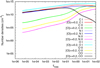 |
Fig. 1 Changes of species number densities in the solar atmosphere due to an increase of the oxygen abundance of 0.2 dex. |
Response of the oxygen abundances in the solar atmosphere to various carbon abundances.
3.8 Problems with CH lines in the blue spectral region
Some authors use CH band heads at 4300 Å to determine the carbon abundance from the fits to the spectral feature as well as single CH lines across the blue spectral region (see Alexeeva & Mashonkina 2015; Suárez-Andrés et al. 2017). Indeed, in the case of a well-determined continuum, such as in the solar case for instance, we obtain good agreement between results obtained with the fits to atomic lines + C2 and CH lines, which is in good agreement with Alexeeva & Mashonkina (2015).
However, in our case of metal-rich stars, blending becomes stronger in the blue part of the spectrum. Therefore, continuum determination becomes more complicated. Furthermore, in many cases, the S/N decreases toward the blue end of the spectrum. Some of our stars have a V sin i > 4 km s −1, increasing the uncertainty in the continuum level determination. Any inaccurate continuum determination in the blue part of the HARPS spectra results in differences of abundances determined from the fits to the CH and C2 + C I absorption lines. The same problem was noted by Ivanyuk et al. (2017) who did not use the lines from the blue part of the CHEPS spectra. To reduce the uncertainties caused by problems with continuum determination in the blue part of the spectrum, we excludedCH lines from our analysis.
4 Results
4.1 V sin i versus mass
Using empirical formulas of the dependence of mass versus luminosity for solar-like stars (Eker et al. 2015), we computed masses for all the stars of our sample. In this case we used the luminosities provided by the Gaia DR2 (Gaia Collaboration 2018). As mentioned above, we used the V sin i determined in the recent paper by Ivanyuk et al. (2017) from the fits to Fe I line profiles.
We show the dependence of V sin i on stellar masses in Fig. 2. The rate of rotational momentum loss should depend on the mass of the star, i.e. more massive stars should remain fast rotators on longer timescales. Indeed, we confirm the dependence empirically (see Fig. 2).
A linear approximation for the dependence of V sin i on M*∕M⊙ is described by the formulae V sin i = (4.68 ± 0.65) × (M*∕M⊙) − 2.06 ± 0.74 for the non-SWP stars and (9.09 ± 1.56) × (M*∕M⊙) − 7.08 ± 1.793 for the SWP stars; see blue and red lines in Fig. 2, respectively.
Likely, rates of angular momentum losses are lower for more massive stars. We do not see any fast rotator at the low-mass end of our sample. The presence of more massive stars with lower V sin i can also be explained by a low sin i factor, rather than a low value of V.
Rates of angular momentum loss are different in SWP and non-SWP. The averaged slope of the dependence of V sin i versus M* is steeper for the non-SWP stars. It appears that the low-mass SWP lose their angular momentum more efficiently than low-mass non-SWP. Naturally, masses and angular momenta of proto-planetary discs are different. However, most of our stars have evolved far enough from their time of planet formation for this to be an issue; also our SWP should have massive enough protoplanetary discs to form objects of planetary masses. For more detailed analysis, we should carefully consider all observations made at high accuracy for all planetary systems of our SWP. This task is beyond the scope of this paper. Therefore, our conclusion is rather qualitative; we observe a tendency toward lower angular momentum for SWP in comparison to non-SWP.
It is worth noting that in this case the samples of SWP and non-SWP stars are different in numbers. Our sample of SWP stars is less presentable, therefore errors are larger in comparison with the non-SWP stars. For more confident conclusions, analyses of a larger number of stars are required.
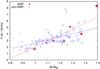 |
Fig. 2 Measured rotational velocities vs. stellar mass. Symbols sizes are a function of stellar masses, given in solar masses M⊙. |
4.2 Comparison to other authors
In general, we obtained good agreement with other authors. Because we have the same input line lists and other parameters well-defined, i.e. effective temperature, gravity, and abundances of other elements, our results of the carbon abundance determination agree with Alexeeva & Mashonkina (2015) better than 0.05 dex for the Sun, despite some differences in the used procedure and model atmospheres. We obtain similar trends of [C/H] versus [Fe/H] in Nissen et al. (2014, see their Fig. 11), or Suárez-Andrés et al. (2017, see their Fig. 5).
In the case of the oxygen abundance results, the overall situation seems to be more complicated. We found 10 stars in common with Bensby et al. (2014), which are listed in the Table 4. However, Bensby et al. (2014) used the near-infrared multiplet lines of O I at 7771.94, 7774.17 and 7775.39 Å, which are known to be affected by NLTE effects (see Kiselman 1993; Asplund et al. 2009). Bensby et al. (2014) used empirical formula to account for the NLTE corrections of O I abundances.In this paper we used the O I line at 6300.304 Å, which is less affected by NLTE effects. On the other hand, this line is much weaker in comparison to the near-infrared multiplet lines and forms a blend with a notable Ni I line; see Sect. 3.5. Differences of the formally determined abundances may be on the order of 0.15 dex or even exceed this value (Bensby et al. 2004, see Table 3). Strictly speaking, the use of 6300.304 Å for O I abundance determination is possible only in the case of known Ni abundance in the stellar atmosphere. Fortunately, in this paper we used Ni abundances in the atmospheres of our stars determined by Ivanyuk et al. (2017). Nevertheless, a direct comparison of our oxygen abundances for 8 out of the 10 overlapping stars agree within ±0.05 dex, despite all differences in the input spectra and applied procedures for the abundance determination. The notable differences for 2 stars (NN = 2 and 9, see Table 4) might be caused by cumulative effects of differences in the adopted Teff, log g, Vt. Besides, these stars are relatively fast rotators (V sin i = 4.1 and 3.5 km s−1) in comparison to other common stars; see Table 4. The procedure of the formal approximation of the line profile by Gaussianor even Voigt functions used by Bensby et al. (2014) might not work correctly in some cases. Indeed, the rotational profile cannot be fitted by any Gaussian (Gray 1976).
In any case, formally our oxygen abundances agree within the uncertainties determined by Bensby et al. (2014). De facto agreement in our abundances with Bensby et al. (2014) for slowly rotating common stars is notably better (see Fig. 3). It is worth noting that the comparison with Bensby et al. (2014) was carried out only to compare how the results were affected by the cumulative effects of differences in the procedure used, methods, and input data. To perform a more detailed comparison, we should follow all the analysis steps they performed very precisely, i.e. following the same line lists, damping constants, chemical equilibrium details, etc. as in Ivanyuk et al. (2017).
Comparison of the oxygen abundances in this work and Bensby et al. (2014).
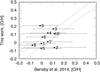 |
Fig. 3 Comparison of our oxygen abundances with Bensby et al. (2014) for the common stars. Dashed lines indicate the difference of abundances in ±0.05 dex from the line of equal values. |
4.3 Oxygen and carbon abundance in the CHEPS stars
The abundances of C and O in the atmospheres of all stars of our sample are shown in Table A.3. The O I line 6300.304 Å isseverely blended by telluric lines in the spectra of five stars. For these stars we provide oxygen abundances scaled from the iron abundance, these cases are marked by (*) in Table A.3. A histogram of the C and O abundance distributions is shown in Fig. 4.
We notice that the histogram is broader and slightly shifted for oxygen with a full width at half maximum (FWHM) of 0.4 for [O/Fe] rather than 0.3 for [C/Fe]. Thus, oxygen is somewhat more abundant at lower metallicities relative to carbon. It is likely that, if the metallicity reflects the age of the stars, we are seeing the results of the differing efficiency of C and O production at different times of the evolution of the Galaxy.
In Fig. 5 we show the dependence of [O/H] and [C/H] versus [Fe/H] in atmospheres of our stars. We found a notable dispersion (±0.15 dex) of the C and O abundances. Likely, the dispersion is intrinsic. In general, both C and O abundances follow the metallicity. Furthermore, there is no particular dependence of C and O abundance on mass.
The solar C and O abundances are always on the averaged trend. In other words, we do not see any peculiarity of the Sun in comparison to other stars of our sample.
Averaged trends of oxygen and carbon abundances versus metallicity show similar trends for both SWP and non-SWP. However, in both cases the averaged trend for non-SWP stars looks steeper. The difference is more pronounced in the analysis of [C/O]; see Sects. 4.4 and 4.5.
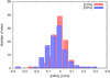 |
Fig. 4 [C/Fe] and [O/Fe] histograms for the sample of CHEPS stars, shown by different colours. |
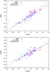 |
Fig. 5 [C/H] and [O/H] vs. [Fe/H]. The SWP are shown with red circles. Larger circles indicate the stars of larger masses. The asteriskmarks the Sun. |
4.4 [C/O] versus [Fe]
The differences between SWP and non-SWP are better seen in Fig. 6. We show the dependence of [C/O] versus [Fe]. The differences between the averaged trends of the dependence are at the level of 0.05 dex; most of our SWP have [C/O] > 0, i.e. most of them are carbon rich in comparison to the solar case.
At least three stars, i.e. HIP 29442, HIP 51987, and HIP 69724 seen in the right bottom part of the Fig. 5, manifest a difference of [C/O] from other stars that is too large. We note that only in the case of one star, HIP 29442, is its O I line severely blended by the telluric line, which makes the oxygen abundance determination very problematic; see Fig. A.2 and Sect. 3.5. Two other stars, HIP 51987 and HIP 69724, show rather “normal” carbon abundances log N(C) = −3.23, −3.20, but log N(O) = −2.57 and −2.59, respectively (see Table A.3). We suggest performing more detailed study of these stars in the near future.
In total, we have 10 problematic stars with the poorly determined oxygen abundances, see Table A.3. In spectra of five stars, the O I line profile is only partially affected by blending with telluric lines and/or “bad pixels”. Their oxygen abundances, indicated by (+), were determined “by hands”, i.e. from visual comparison of computed and observed spectra.
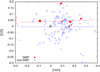 |
Fig. 6 Dependence [C/O] vs. [Fe/H]. The SWP are shown with red circles. Larger circles indicate the stars of larger masses. Error bars from the determinations of the mean [C/O] in the samples of SWP and non-SWP are shown by the red and blue arrows. Linear approximation results for the SWP and non-SWP stars shown by red ([C/O] = ((−0.576 ± 0.273) ⋅ [Fe∕H] + 0.047 ± 0.0158) and blue ([C/O] = (0.759 ± 0.077) ⋅ [Fe∕H] + 0.0079 ± 0.006) lines, respectively. |
4.5 [C/O] versus V sin i
Generally speaking, a fast rotation may affect the processes of matter transfer in the interiors of the star, which could give rise to a dependence of [C/O] versus V sin i. However, our results do not confirm this suggestion: in Fig. 7 we see only a slight increase of [C/O] toward larger V sin i. However, our stars are comparatively slow rotators by selection, therefore this hypothesis should be tested on a larger sample of stars across a wider range of V sin i.
On the other hand, we see the results discussed in Sect. 4.1. Namely, almost all our massive stars occupy the range of V sin i > 3 km s −1, regardless of whether they are SWP or non-SWP.
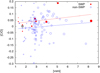 |
Fig. 7 [C/O] versus V sin i. The Sun is marked by an asterisk. More massive stars are labelled by circles of larger radius. Linear approximation of results for the SWP and non-SWP stars shown by red ([C/O] = (0.009 ± 0.008) × V sin i + 0.0140 ± 0.033) and blue ([C/O] = (0.007 ± 0.008) × V sin i-0.0271 ± 0.028) lines, respectively. |
4.6 Lithium versus oxygen
Lithium is an element of special interest in many aspects of modern astrophysics (see Pavlenko et al. 2018 and references therein). Li is a fragile element; theoretical models predict lithium depletion that can be compared to the lithium in the Sun and stars of different ages and metallicities. Piau & Turck-Chièze (2002) distinguished two phases in lithium depletion: (1) a rapid nuclear destruction in the T Tauri phase before 20 Myr in stars of 0.8 and 1.4 M⊙ masses, which is dependent on the extent and temperature of the convective zone, and (2) a second phase in which the destruction is slow and moderate and is largely dependent on the (magneto)hydrodynamic instability located at the base of the convective zone. Piau & Turck-Chièze (2002) outlined the importance of the O/Fe ratio due to the role of oxygen as known source of opacity.
To investigate the problem of the possible dependence of the lithium abundance versus the oxygen abundance, we used the results of the Li determinations by Pavlenko et al. (2018), where the dependence of N(Li) versus N(O) is shown in Fig. 8 for all stars of our sample, i.e. with detectable Li and the upper limits of lithium abundances. It is clear thatour sample is not complete enough to provide a firm conclusion, but there the notable connection between thelithium and oxygen abundances does appear; this is shown by the red line in Fig. 8, i.e. log N(Li) = 2.16 ± 0.07 − (1.67 ± 0.9) ⋅ [O/Fe]. The slope ofthe dependence is determined with a large error bar, but it is negative in this case, in accordance with the prediction of Piau & Turck-Chièze (2002). Interestingly, all four of our SWP are found to have lithium abundances above the mean linear fit to the data.
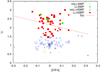 |
Fig. 8 [Li] vs. [O] for stars with a detectable lithium 6708 Å line and the upper limit of lithium abundances in stars of our sample. TheSun is marked by an asterisk. More massive stars are labelled by figures of larger radius. |
4.7 O and C in stars of different ages
Using the luminosities of our stars from the Gaia DR2 along with the recent evolutionary tracks from the the Modules for Experiments in Stellar Astrophysics (MESA) Isochrones and Stellar Tracks (MIST) project described in detail by Dotter (2016), Choi et al. (2016), and Paxton et al. (2011, 2013, 2015), we determined the ages of our stars. Generally speaking, measuring the ages of low-mass stars to high precision is difficult, particularly old Sun-like stars on the main sequence, where evolutionary model convergence can give rise to large uncertainties. Low-mass stars, i.e. stars of solar masses or smaller, evolve very slowly, such that their luminosities increase slowly with time, as seen in Fig. A.5. Furthermore, the evolution of stars notably depends on their metallicities, whereby metal-deficient stars are generally of a higher luminosity, and therefore they evolve in shorter timescales. Uncertainties in the metallicity of ±0.2 dex can give rise to an uncertainty of ±2 Myr in age for a star of solar mass. We computed evolutionary tracks of our stars for their masses and metallicities given in the Table A.3 using the web interpolator3 of the MISTdatabase. The comparison of the observed luminosities and theoretical MIST luminosities are available on web4. The ages of our stars are given in the Table A.3. We note that for some stars, we cannot find proper solutions, meaning their calculated ages exceed Hubbletime, i.e. >14 Gyr. We highlight these stars in our plots to underline the existing problems in age determinations using the latest and most up-to-date evolutionary tracks. In any case, the majority of these “strange” stars are of masses lower than 1 M⊙. Detailed analysis of these results is beyond the scope of this paper, but is an avenue that should be explored further in the future.
Nevertheless, we show the dependence [C/Fe] and [O/Fe] versus age in Figs. A.6 and A.7, respectively.In both cases we see rather positive slopes of the dependences. It can be interpreted as evidence that at older times, production of C and O prevails over Fe yield.
5 Discussion
We carried out our analysis in the framework of the classical approach. Since the stars of our sample are dwarfs, we employed the simplifications of using LTE, 1D, and no sinks and energy sources in the atmosphere, therefore the mixing-length theory of convection is still valid for our model computations. Indeed, for the case of the solar atmosphere we obtain a good agreement with other authors for the investigated abundances, Vt and V sin i.
In this paper we adopted the Anders & Grevesse (1989) abundance scale. This was done only to fix the “zero point” in our computations. Generally speaking, we performed our abundance and other parameter analyses relative to the Sun. In other words, our procedure was adopted for the Sun, and then later we performed the same analysis on other stars. Our analysis shows that the Sun can be considered a normal star in this respect, since its parameters correspond well to the average parameters of the stars in our sample.
In the framework of the project, we determine masses of all stars of our sample using luminosities provided by the second data release of Gaia, allowing us to add one more dimension to our analysis. At least ten of our stars are SWP. The comparison of SWP and non-SWP provides another interesting aspect of our research. It is worth noting that the analysis of SWP and non-SWP was carried out in the framework of the same approach. In other words, all abundances and other parameters were determined using fits to the observed spectra observed by one instrument and the same analysis procedure was employed.
Despite the problems of age determination of G dwarfs, we computed the ages of the stars of our sample using the comparison of Gaia DR2 luminosities with the MIST evolutionary tracks. The accuracy of age determination of lower mass stars seems to be controversial in many cases though both dependencies [C/Fe] and [O/Fe] versus age are positive. Likely, the production of C and O was more effective in comparison with Fe in former epochs.
Usually, in abundance analysis we used many lines to reduce possible formal errors. In the case of the oxygen abundance determination we used only one line at 6300.304 Å. However, this line has been studied in detail by many authors (see Allende Prieto et al. 2001). The line blends with the Ni I line at 6300.336 Å, which practically means the use of the 6300.304 Å line is restricted to cases where the Ni abundance is known. Fortunately, the Ni abundance in the stars of our sample was previously determined (Ivanyuk et al. 2017). Furthermore, we adjusted the parameters of the Ni line to obtain the known solar abundance (Anders & Grevesse 1989). This allows us to reproduce the O I and Ni I line blend in the solar spectrum. We do not use the 6363 Å line because of its weakness. Unfortunately, even small uncertainties across weak spectral lines reduce the accuracy of abundance determination from the fit to this line. Other important input parameters, i.e. effective temperatures, gravities, micro-, and microturbulent velocities were taken from Ivanyuk et al. (2017).
Carbon abundances were determined using the list of C I and C2 lines from the paper of Alexeeva & Mashonkina (2015). Our results for the Sun agree well with these authors within ±0.02 dex, despite the differences in model atmospheres, procedures, etc. We do not use lines from the CH molecule that appear in the blue spectral region owing to strong blending there that affects the continuum determination. The V sin i for all stars of our sample was determined by Ivanyuk et al. (2017), and we found that most of our fast rotators are more massive stars.
From our analysis we do not find evidence that the [C/O] ratio depends on V sin i or mass of the star. We do not find any correlation between [C/O] and the lithium abundance. On the other hand, we see a large dispersion of C and O abundances for the stars of different masses and metallicities. Even if we could explain some of the observed dispersion of oxygen from the use of only a single line, the problem of the abundance dispersion still remains for carbon, which was determined by the analysis of a large enough number of atomic and molecular lines. Despite the notable dispersion of C and O abundances, our histogram analysis showed some differences in the distribution of these species.
In general, carbon and oxygen abundances follow metallicity. However, the comparison between their overall distributions show that more oxygen is formed at lower metallicities, whereas carbon formation is more effective at higher metallicities, and hence later times, if metallicity reflects the time of formation of the star. Thus, carbon production is more effective at later epochs in the evolution of the Milky Way. In this way we see the slightly different abundance histories of oxygen and carbon in our Galaxy.
We note that FHWMs of [C/Fe[and [O/Fe] distributions in atmospheres of stars of our sample are subtly different and oxygen production is somewhat favoured at lower metallicities relatively to carbon. Our targets are mainly G dwarfs, which cannot easily change their surface abundances of oxygen and carbon on short timescales. This presumably arises from the differences in the processes yielding C and O at different metallicities during the evolution of our Galaxy for which is some evidence from other work (e.g. Chiappini et al. 2003).
Finally, we confirm that SWP are more carbon rich in comparison with non-SWP, in agreement with, for example Suárez-Andrés et al. (2017). It is worth noting that this result was obtained from analysis of only 10 SWP and 97 non-SWP stars. On the other hand, our analysis was done in the framework of a homogeneous set of the observed data, all using the same procedure. Therefore, this abundance difference between SWP and non-SWP is real. At least, the shift between averaged [C/O] for the samples of SWP and non-SWP exceeds the formal error bars determined for these samples.
We carry out numerical Monte Carlo simulations of the [C/Fe] distributions to estimate the reality of the computed differences for SWP and non-SWP; see Fig. A.4. Random numbers were generated by the RANDOM_NUMBERS procedure of Fortran 95, and an extended set of Monte Carlo simulations (N = 108) was carried out, drawing from normal distributions of the [C/Fe] abundance ratio in both SWP and non-SWP samples. We used a normal distribution based on the results for [C/Fe] we found in Fig. 4. We found a probability of the null result of only 3.9%. In other words, there is a 96.1% probability that the populations are drawn from different parent distributions, a value approaching 3σ.
Acknowledgments
We acknowledge support by Fondecyt grant 1161218 and partial support by CATA-Basal (PB06, CONICYT) and support from the UK STFC via grants ST/M001008/1. Y.P. has been supported in part by grant from the Polish National Science Center 2016/21/B/ST9/01626. Special thanks to developers of the MIST evolutionary tracks database. We thank the anonymous referee for a thorough review and we highly appreciate the comments and suggestions, which significantly contributed to improving the quality of the publication.
Appendix A: Additional figures and tables
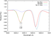 |
Fig. A.1 Contribution of O I, Ni I and other lines into the formation of the 6300.304 Å line in the solar spectrum. |
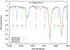 |
Fig. A.2 Spectral range around the O I λ 6300.304 Å line observed for three stars of our CHEPS sample. Telluric O2 lines are indicated by arrows. |
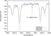 |
Fig. A.3 Spectral range around the O I λ 6363.776 Å line observed for three stars of our CHEPS sample. |
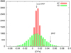 |
Fig. A.4 Distributions are mean [C/Fe] for SWP (N = 10) and non-SWP (N = 97) points for 10 000 simulations. The arrows indicate our mean results for SWP and non-SWP from observations, respectively. |
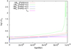 |
Fig. A.5 Comparison of the theoretical evolutionary luminosity tracks of stars of the one solar mass of different [Fe/H] = −0.2, 0.0, +0.1 and +0.2. |
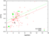 |
Fig. A.6 [C/Fe] vs. age of CHEPS stars. The stars with and without planets are shown by green and red colours, respectively.Symbols sizes are proportional to the stellar masses. The asterisk indicates the Sun. |
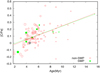 |
Fig. A.7 [O/Fe] vs. age of CHEPS stars. The stars with and without planets are shown by green and red colours, respectively.Symbols sizes are proportional to the stellar masses. The asterisk indicates the Sun. |
Spectroscopic parameters of the absorption lines that form the 6300.3 Å feature.
Abundances of carbon in solar atmosphere, determined from a selected lines of the CCS.
Carbon and oxygen in the CHEPS stars.
References
- Alexeeva, S. A., & Mashonkina, L. I. 2015, MNRAS, 453, 1619 [NASA ADS] [CrossRef] [Google Scholar]
- Allende Prieto, C., Lambert, D. L., & Asplund, M. 2001, ApJ, 556, L63 [NASA ADS] [CrossRef] [Google Scholar]
- Anders, E., & Grevesse, N. 1989, Geochim. Cosmochim. Acta, 53, 197 [Google Scholar]
- Asplund, M., Grevesse, N., Sauval, A. J., Allende Prieto, C., & Blomme, R. 2005, A&A, 431, 693 [NASA ADS] [CrossRef] [EDP Sciences] [Google Scholar]
- Asplund, M., Grevesse, N., Sauval, A. J., & Scott, P. 2009, ARA&A, 47, 481 [NASA ADS] [CrossRef] [Google Scholar]
- Bensby, T., Feltzing, S., & Lundström, I. 2004, A&A, 415, 155 [NASA ADS] [CrossRef] [EDP Sciences] [Google Scholar]
- Bensby, T., Feltzing, S., & Oey, M. S. 2014, A&A, 562, A71 [NASA ADS] [CrossRef] [EDP Sciences] [Google Scholar]
- Bertran de Lis, S., Delgado Mena, E., Adibekyan, V. Z., Santos, N. C., & Sousa, S. G. 2015, A&A, 576, A89 [NASA ADS] [CrossRef] [EDP Sciences] [Google Scholar]
- Bond, J. C., Lauretta, D. S., & O’Brien, D. P. 2010a, Icarus, 205, 321 [NASA ADS] [CrossRef] [Google Scholar]
- Bond, J. C., O’Brien, D. P., & Lauretta, D. S. 2010b, ApJ, 715, 1050 [NASA ADS] [CrossRef] [Google Scholar]
- Caimmi, R. 2011, Serbian Astron. J., 183, 37 [NASA ADS] [CrossRef] [Google Scholar]
- Chiappini, C., Romano, D., & Matteucci, F. 2003, MNRAS, 339, 63 [NASA ADS] [CrossRef] [Google Scholar]
- Choi, J., Dotter, A., Conroy, C., et al. 2016, ApJ, 823, 102 [NASA ADS] [CrossRef] [Google Scholar]
- Covey, K. R., Hawley, S. L., Bochanski, J. J., et al. 2008, AJ, 136, 1778 [NASA ADS] [CrossRef] [Google Scholar]
- de Kool, M., & Green, P. J. 1995, ApJ, 449, 236 [NASA ADS] [CrossRef] [Google Scholar]
- Delgado Mena, E., Israelian, G., González Hernández, J. I., et al. 2010, ApJ, 725, 2349 [NASA ADS] [CrossRef] [Google Scholar]
- Dotter, A. 2016, ApJS, 222, 8 [NASA ADS] [CrossRef] [Google Scholar]
- Downes, R. A., Margon, B., Anderson, S. F., et al. 2004, AJ, 127, 2838 [NASA ADS] [CrossRef] [Google Scholar]
- Ecuvillon, A., Israelian, G., Santos, N. C., et al. 2004, A&A, 426, 619 [NASA ADS] [CrossRef] [EDP Sciences] [Google Scholar]
- Ecuvillon, A., Israelian, G., Santos, N. C., et al. 2006, A&A, 445, 633 [NASA ADS] [CrossRef] [EDP Sciences] [Google Scholar]
- Eker, Z., Soydugan, F., Soydugan, E., et al. 2015, AJ, 149, 131 [NASA ADS] [CrossRef] [Google Scholar]
- Fortney, J. J. 2012, ApJ, 747, L27 [NASA ADS] [CrossRef] [Google Scholar]
- Gaia Collaboration (Brown, A. G. A., et al.) 2018, A&A, 616, A1 [NASA ADS] [CrossRef] [EDP Sciences] [Google Scholar]
- Gray, D. F. 1976, The Observation and Analysis of Stellar Photospheres (Cambridge: Cambridge University Press) [Google Scholar]
- Gustafsson, B., Karlsson, T., Olsson, E., Edvardsson, B., & Ryde, N. 1999, A&A, 342, 426 [NASA ADS] [Google Scholar]
- Haywood, M. 2001, MNRAS, 325, 1365 [NASA ADS] [CrossRef] [Google Scholar]
- Ivanyuk, O. M., Jenkins, J. S., Pavlenko, Y. V., Jones, H. R. A., & Pinfield, D. J. 2017, MNRAS, 468, 4151 [NASA ADS] [CrossRef] [Google Scholar]
- Jenkins, J. S., Jones, H. R. A., Pavlenko, Y., et al. 2008, A&A, 485, 571 [NASA ADS] [CrossRef] [EDP Sciences] [Google Scholar]
- Jenkins, J. S., Ramsey, L. W., Jones, H. R. A., et al. 2009, ApJ, 704, 975 [NASA ADS] [CrossRef] [Google Scholar]
- Jenkins, J. S., Murgas, F., Rojo, P., et al. 2011, A&A, 531, A8 [NASA ADS] [CrossRef] [EDP Sciences] [Google Scholar]
- Jenkins, J. S., Jones, H. R. A., Tuomi, M., et al. 2017, MNRAS, 466, 443 [NASA ADS] [CrossRef] [Google Scholar]
- Kiselman, D. 1993, A&A, 275 [Google Scholar]
- Kurucz, R. L., Furenlid, I., Brault, J., & Testerman, L. 1984, Solar Flux Atlas from 296 to 1300 nm (Sunsport, NM: National Solar Observatory) [Google Scholar]
- Mayor, M., Pepe, F., Queloz, D., et al. 2003, The Messenger, 114, 20 [NASA ADS] [Google Scholar]
- Murgas, F., Jenkins, J. S., Rojo, P., Jones, H. R. A., & Pinfield, D. J. 2013, A&A, 552, A27 [NASA ADS] [CrossRef] [EDP Sciences] [Google Scholar]
- Nissen, P. E., Chen, Y. Q., Carigi, L., Schuster, W. J., & Zhao, G. 2014, A&A, 568, A25 [NASA ADS] [CrossRef] [EDP Sciences] [Google Scholar]
- Pantoja, B. M., Jenkins, J. S., Girard, J. H., et al. 2018, MNRAS, 479, 4958 [NASA ADS] [CrossRef] [Google Scholar]
- Pavlenko, Y. V. 2003, Astron. Rep., 47, 59 [NASA ADS] [CrossRef] [Google Scholar]
- Pavlenko, Y. V. 2017, Kinemat. Phys. Celest. Bodies, 1, 55 [NASA ADS] [CrossRef] [Google Scholar]
- Pavlenko, Y. V., Jenkins, J. S., Jones, H. R. A., Ivanyuk, O., & Pinfield, D. J. 2012, MNRAS, 422, 542 [NASA ADS] [CrossRef] [Google Scholar]
- Pavlenko, Y. V., Jenkins, J. S., Ivanyuk, O. M., et al. 2018, A&A, 611, A27 [NASA ADS] [CrossRef] [EDP Sciences] [Google Scholar]
- Paxton, B., Bildsten, L., Dotter, A., et al. 2011, ApJS, 192, 3 [Google Scholar]
- Paxton, B., Cantiello, M., Arras, P., et al. 2013, ApJS, 208, 4 [NASA ADS] [CrossRef] [Google Scholar]
- Paxton, B., Marchant, P., Schwab, J., et al. 2015, ApJS, 220, 15 [Google Scholar]
- Petigura, E. A., & Marcy, G. W. 2011, ApJ, 735, 41 [NASA ADS] [CrossRef] [Google Scholar]
- Piau, L., & Turck-Chièze, S. 2002, ApJ, 566, 419 [NASA ADS] [CrossRef] [Google Scholar]
- Ryabchikova, T., Piskunov, N., Kurucz, R. L., et al. 2015, Phys. Scr, 90, 054005 [NASA ADS] [CrossRef] [Google Scholar]
- Searle, L., & Sargent, W. L. W. 1972, ApJ, 173, 25 [NASA ADS] [CrossRef] [Google Scholar]
- Soto, M. G., & Jenkins, J. S. 2018, A&A, 615, A76 [NASA ADS] [CrossRef] [EDP Sciences] [Google Scholar]
- Suárez-Andrés, L., Israelian, G., González Hernández, J. I., et al. 2017, A&A, 599, A96 [NASA ADS] [CrossRef] [EDP Sciences] [Google Scholar]
- Suárez-Andrés, L., Israelian, G., González Hernández, J. I., et al. 2018, A&A, 614, A84 [NASA ADS] [CrossRef] [EDP Sciences] [Google Scholar]
- Valenti, J. A.,& Piskunov, N. 1996, A&AS, 118, 595 [NASA ADS] [CrossRef] [EDP Sciences] [Google Scholar]
- Worthey, G., Dorman, B., & Jones, L. A. 1996, AJ, 112, 948 [NASA ADS] [CrossRef] [Google Scholar]
All Tables
Response of the oxygen abundances in the solar atmosphere to various carbon abundances.
Spectroscopic parameters of the absorption lines that form the 6300.3 Å feature.
Abundances of carbon in solar atmosphere, determined from a selected lines of the CCS.
All Figures
|
Fig. 1 Changes of species number densities in the solar atmosphere due to an increase of the oxygen abundance of 0.2 dex. |
| In the text | |
|
Fig. 2 Measured rotational velocities vs. stellar mass. Symbols sizes are a function of stellar masses, given in solar masses M⊙. |
| In the text | |
|
Fig. 3 Comparison of our oxygen abundances with Bensby et al. (2014) for the common stars. Dashed lines indicate the difference of abundances in ±0.05 dex from the line of equal values. |
| In the text | |
|
Fig. 4 [C/Fe] and [O/Fe] histograms for the sample of CHEPS stars, shown by different colours. |
| In the text | |
|
Fig. 5 [C/H] and [O/H] vs. [Fe/H]. The SWP are shown with red circles. Larger circles indicate the stars of larger masses. The asteriskmarks the Sun. |
| In the text | |
|
Fig. 6 Dependence [C/O] vs. [Fe/H]. The SWP are shown with red circles. Larger circles indicate the stars of larger masses. Error bars from the determinations of the mean [C/O] in the samples of SWP and non-SWP are shown by the red and blue arrows. Linear approximation results for the SWP and non-SWP stars shown by red ([C/O] = ((−0.576 ± 0.273) ⋅ [Fe∕H] + 0.047 ± 0.0158) and blue ([C/O] = (0.759 ± 0.077) ⋅ [Fe∕H] + 0.0079 ± 0.006) lines, respectively. |
| In the text | |
|
Fig. 7 [C/O] versus V sin i. The Sun is marked by an asterisk. More massive stars are labelled by circles of larger radius. Linear approximation of results for the SWP and non-SWP stars shown by red ([C/O] = (0.009 ± 0.008) × V sin i + 0.0140 ± 0.033) and blue ([C/O] = (0.007 ± 0.008) × V sin i-0.0271 ± 0.028) lines, respectively. |
| In the text | |
|
Fig. 8 [Li] vs. [O] for stars with a detectable lithium 6708 Å line and the upper limit of lithium abundances in stars of our sample. TheSun is marked by an asterisk. More massive stars are labelled by figures of larger radius. |
| In the text | |
|
Fig. A.1 Contribution of O I, Ni I and other lines into the formation of the 6300.304 Å line in the solar spectrum. |
| In the text | |
|
Fig. A.2 Spectral range around the O I λ 6300.304 Å line observed for three stars of our CHEPS sample. Telluric O2 lines are indicated by arrows. |
| In the text | |
|
Fig. A.3 Spectral range around the O I λ 6363.776 Å line observed for three stars of our CHEPS sample. |
| In the text | |
|
Fig. A.4 Distributions are mean [C/Fe] for SWP (N = 10) and non-SWP (N = 97) points for 10 000 simulations. The arrows indicate our mean results for SWP and non-SWP from observations, respectively. |
| In the text | |
|
Fig. A.5 Comparison of the theoretical evolutionary luminosity tracks of stars of the one solar mass of different [Fe/H] = −0.2, 0.0, +0.1 and +0.2. |
| In the text | |
|
Fig. A.6 [C/Fe] vs. age of CHEPS stars. The stars with and without planets are shown by green and red colours, respectively.Symbols sizes are proportional to the stellar masses. The asterisk indicates the Sun. |
| In the text | |
|
Fig. A.7 [O/Fe] vs. age of CHEPS stars. The stars with and without planets are shown by green and red colours, respectively.Symbols sizes are proportional to the stellar masses. The asterisk indicates the Sun. |
| In the text | |
Current usage metrics show cumulative count of Article Views (full-text article views including HTML views, PDF and ePub downloads, according to the available data) and Abstracts Views on Vision4Press platform.
Data correspond to usage on the plateform after 2015. The current usage metrics is available 48-96 hours after online publication and is updated daily on week days.
Initial download of the metrics may take a while.