| Issue |
A&A
Volume 620, December 2018
|
|
|---|---|---|
| Article Number | A91 | |
| Number of page(s) | 4 | |
| Section | Planets and planetary systems | |
| DOI | https://doi.org/10.1051/0004-6361/201834007 | |
| Published online | 30 November 2018 | |
Reconstruction of asteroid spin states from Gaia DR2 photometry★
Astronomical Institute, Faculty of Mathematics and Physics, Charles University, V Holešovičkách 2,
180 00 Prague 8, Czech Republic
e-mail: This email address is being protected from spambots. You need JavaScript enabled to view it.
Received:
3
August
2018
Accepted:
21
September
2018
Abstract
Context. In addition to stellar data, Gaia Data Release 2 (DR2) also contains accurate astrometry and photometry of about 14 000 asteroids covering 22 months of observations.
Aims. We used Gaia asteroid photometry to reconstruct rotation periods, spin axis directions, and the coarse shapes of a subset of asteroids with enough observations. One of our aims was to test the reliability of the models with respect to the number of data points and to check the consistency of these models with independent data. Another aim was to produce new asteroid models to enlarge the sample of asteroids with known spin and shape.
Methods. We used the lightcurve inversion method to scan the period and pole parameter space to create final shape models that best reproduce the observed data. To search for the sidereal rotation period, we also used a simpler model of a geometrically scattering triaxial ellipsoid.
Results. By processing about 5400 asteroids with at least 10 observations in DR2, we derived models for 173 asteroids, 129 of which are new. Models of the remaining asteroids were already known from the inversion of independent data, and we used them for verification and error estimation. We also compared the formally best rotation periods based on Gaia data with those derived from dense lightcurves.
Conclusions. We show that a correct rotation period can be determined even when the number of observations N is less than 20, but the rate of false solutions is high. For N > 30, the solution of the inverse problem is often successful and the parameters are likely to be correct in most cases. These results are very promising because the final Gaia catalogue should contain photometry for hundreds of thousands of asteroids, typically with several tens of data points per object, which should be sufficient for reliable spin reconstruction.
Key words: minor planets, asteroids: general / methods: data analysis / techniques: photometric
Table A.1 is only available at the CDS via anonymous ftp to cdsarc.u-strasbg.fr (130.79.128.5) or via http://cdsarc.u-strasbg.fr/viz-bin/qcat?J/A+A/620/A91
© ESO 2018
1 Introduction
The ESA Gaia mission (Gaia Collaboration 2016a) has been in the science operations phase since August 2014. So far, there have been two Data Releases, the first in September 2016 (DR1, Gaia Collaboration 2016b) and the second in April 2018 (DR2, Gaia Collaboration 2018a). The main output of DR2 is accurate astrometric data for more than a billion stars. However, unlike DR1, DR2 also contains astrometric and photometric data for about 14 000 asteroids (Gaia Collaboration 2018b).
Time-resolved photometry of asteroids, i.e. lightcurves, can be used for the reconstruction of the rotation period, spin axis orientation, and shape (Kaasalainen et al. 2002; Michałowski et al. 2004; Ďurech et al. 2007a; Marciniak et al. 2007, 2018; Kryszczyńska 2013; Hanuš et al. 2016, for example). Also, photometry that is sparse in time with respect to the rotation period can be successfully used with the same lightcurve inversion method (Kaasalainen 2004; Ďurech et al. 2007b, 2009, 2016; Hanuš et al. 2011, 2013). Gaia provides this type of sparse-in-time photometry with unprecedented accuracy. After the end of mission, these data will be used to determine periods, spins, and triaxial shape models (Cellino et al. 2006, 2007; Cellino & Dell’Oro 2012; Santana-Ros et al. 2015). As shown by Santana-Ros et al. (2015), the probability of deriving a correct spin model is related to the shape (spherical asteroids have small lightcurve amplitudes), spin axis latitude (low-latitude asteroids are sometimes seen pole-on with small lightcurve amplitude), and the number of data points. Until now, real Gaia asteroid photometry was not available and the performance of inversion techniques was tested on simulated data. DR2 has changed this situation and we can now use real high-quality Gaia photometry and test whether the expectations were met. Here we use asteroid photometry released in DR2 with the aim of testing the limits of lightcurve inversion and the information content of the data. We also derive new asteroid models.
2 Inversion of Gaia asteroid photometry
The DR2 contains G-band brightness measurements with uncertainties for about 14 000 asteroids. The observations cover 22 months and the number of data points per object varies from a few to 50. As described by Gaia Collaboration (2018b), the reported brightness values are constant for a single transit and they were computed as average values over the transit. Gaia Collaboration (2018b) also tested the accuracy of the asteroid photometry and reached the conclusion that it is probably better than 1–2%. This is much better than the accuracy of sparse photometry from ground-based surveys, which is hardly better than 0.1 mag (Ďurech et al. 2009). A unique reconstruction of the shape/spin model is possible only if there are enough photometricdata points with good accuracy covering a sufficiently wide interval of geometries. With ground-based surveys, the poor photometric quality is compensated with the number of data points, typically several hundred, observed over many apparitions. Even so, unique solutions are rare; the success rate of deriving a robust and reliable model is less than 1% (Ďurech et al. 2016). In the case of Gaia, the final catalogue will contain data that fulfil all three requirements: they will be very accurate, there will be several tens of measurements per object, and they will cover several apparitions for a typical main-belt asteroid. According to simulations, several tens of accurate measurements should be sufficient to derive a unique spin solution and an approximate shape (Santana-Ros et al. 2015).
DR2 photometry allowed us to test how successful the inversion of real Gaia data is. We selected all 5413 asteroids for which the number of brightness measurements N was ≥ 10. We computed the geometry with respect to the Sun and the Gaia spacecraft for each observation and processed the data in the same way asin Hanuš et al. (2011) and Ďurech et al. (2016, 2018) by using the lightcurve inversion method of Kaasalainen et al. (2001). Our approach is similar to that of Torppa et al. (2018) with the main difference that we do not deal with any error analysis. For each processed asteroid, we searched for a shape/spin model that gives the best fit to the data, measured by the lowest χ2 between the observed and modelled brightness. All data points were given the same weight; we did not take into account errors of individual measurements. The reason was that the relative formal errors are mostly below 2% (90% of all data points), andin this range the difference between, for example, 1% and 0.1% accuracy plays no role because the errors introduced by the model are larger (simplified shape approximation and scattering model assuming uniform albedo).
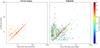 |
Fig. 1 Comparison between the best period derived from Gaia photometry with convex models (left panel) and ellipsoids (right panel). Each point represents an asteroid for which the best-fitting period from Gaia was determined and with a period in the LCDB with the uncertainty code U ≥ 3. The number of Gaia observations N is expressed by the colour. The left panel contains fewer points because convex models were used only when N > 20. |
2.1 Rotation periods
As the first step, we computed periodograms using convex shapes and ellipsoids and tested the reliability of the formally best-fit period. In Fig. 1, we show the comparison between the best period derived from DR2 using either convex shapes or ellipsoids and the values compiled in the Lightcurve Database (LCDB) of Warner et al. (2009); we used the version from November 12, 2017. We used only reliable LCDB periods with the uncertainty code U ≥ 3. The colour-coding correlates with the number of data points N. Convex models do not provide any periods when N ≤ 20 (see the discussion below). The points concentrating on the diagonal line represent the correctly determined periods (Gaia and LCDB periods are the same). The points off the diagonal are likely incorrect Gaia periods because LCDB records with U ≥ 3 should be reliable. The minor diagonal in the left panel are false solutions with the derived period being half of the real one; this can happen with convex shapes as they produce lightcurves with only one minimum/maximum per rotation. Ellipsoidal models do not have this disadvantage of producing false half periods, but the periods based on a small number of points are often wrong. In general, when there are more data points, it is more likely that the derived period will be correct. The clustering of points around shorter periods is likely a consequence of the way the model is constructed; it is easier to formally fit the sparse points with an incorrect period that is shorter than the true period.
The dependence of the number of false periods on the number of data points is shown in Fig. 2. The fraction of correctly determined periods (defined as those that agree with LCDB values within ± 5%) increases above 0.5 when N > 30. For fewer points, the formally best periods are not reliable. For N > 40, the success rate seems to be high, but the sample size of asteroids in this range is very small.
We also tested if there is any difference in the photometric errors of Gaia data between the asteroids with correctly and incorrectly determined rotation periods. For the two bins with N between 21–25 and 26–30 (where the fraction of correctly determined periods is about 50% and the number of periods is large), we compared the photometric errors of points belonging to asteroids with correctly determined periods with those that belong to asteroids with incorrect Gaia-based periods. The t-test did not reveal any significant difference in the means of these two groups. Also, the distribution of observations in time was very similar for the two groups. We did not reveal any statistical difference in, for example, the number of observations separated by 100 min, which is the spacing related to the scanning pattern of Gaia corresponding to two field-of-view transits.
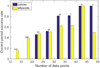 |
Fig. 2 Success rate of deriving correct rotation periods (compared with LCDB) for ellipsoidal and convex models. The number above each histogram bar is the number of asteroids with periods in the LCDB with U ≥ 3 in that interval of data points. |
2.2 Spins and shapes
The best-fit periods discussed above are often just random global minima in the periodograms. To distinguish between random and real periods, we have to define some level of significance measured by the χ2 fit. We defined the uniqueness of the best solution by the depth of the χ2 minimum with respect to other local minima. The formula we used for the threshold 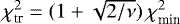 is a modification of the formula we used in Ďurech et al. (2018); now there is no factor of 1/2. This is an arbitrary borderline that is based on a trade-off between the total number of new models and their contamination with incorrect models. Here ν is the number of degrees of freedom, which is formally the difference between the number of points N and the number of parameters p. For ellipsoids, p = 6 and the parameters are the sidereal rotation period P, the spin axis direction in ecliptic coordinates λ and β, one parameter for the linear slope of the phase curve, and two parameters (a∕c and b∕c) for the ellipsoid axes ratios. With Gaia observations the phase angle is almost always > 10°, which means that the phase function can be reduced to only a linear part with one parameter (Kaasalainen et al. 2001). With convex models, we used the spherical harmonics representation of the order and degree of 3 (Kaasalainen et al. 2001), which corresponds to 16 shape parameters, so the total number of parameters is p = 20. For spin/shape reconstruction, we only used asteroids with N > 20.
When the number of points was small, in many cases we obtained RMS residuals of almost zero for many different periods. Such periodograms were excluded from the analysis. To avoid fitting noise, we only selected periodograms with all RMS values > 0.005 mag. Another requirement was that there should be only one period with RMS below 0.01 mag. If there were more, we considered it a non-unique solution even if the threshold limit was satisfied. The verification procedure was the same as in Ďurech et al. (2018), see Fig. 3 there, with the only difference that we did not use n = 6 for the degree and order of the spherical harmonics series. The visual inspection of the periodograms was crucial because in many cases we obtained false solutions for P ≲ 3 h or P ≳ 100 h. Even with a correct rotation period and pole, the corresponding shapes were often unrealistic with sharp edges and triangular pole-on silhouettes. This is a consequence of the order and degree of the spherical harmonics series (n = 3) being too low, but with a small number of photometric points there is not enough information to reconstruct higher resolution models. In this sense, convex shape models derived from DR2 data should not be taken as real shapes; they are just models that fit the data best with the given resolution, and they are likely to change significantly when more data points are available and a higher degree of resolution is possible. On the other hand, the rotation periods and pole directions are not that sensitive to the resolution and they are more reliable (Hanuš & Ďurech 2012).
2.3 Comparison with independent models
By processing all asteroids with N > 20 and rejecting unreliable solutions, we derived models of 173 asteroids. Of these, 44 were already in the Database of Asteroid Models from Inversion Techniques (DAMIT; Ďurech et al. 2010) and we used them for an independent test of the accuracy of our solutions based on DR2. Most of our models agreed with those in DAMIT: their periods were the same within the errorbars and the mean difference between their pole directions was 20°. However, there was a group of clear outliers with differences between pole directions > 60°. We looked in detail into these cases (seven in total). In one case – asteroid (2802) Weisell – the DAMIT model based only on sparse data (Hanuš et al. 2016) was clearly incorrect because the period search was done in the wrong local minimum. We removed this model from DAMIT. In five cases, the periods were very similar but differed more than their uncertainty, so the DR2-based solution wasapparently a different local minimum leading to a different pole. In one case, the periods were completely different.
2.4 New models
In Table A.1, we list 129 new models and their spin axis directions (sometimes there are two possible solutions), the sidereal rotation period, and the period reported in the LCDB. The LCDB period agrees with our value in most cases. The asteroids for which the periods do not agree and the LCDB period is reliable (higher uncertainty code U) are marked with an asterisk.
To further check the reliability of these new models, we repeated the period search using reduced data sets. For each asteroid from Table A.1, we randomly selected and removed 10% of the data points (i.e. 2–5 points) from the original data set. In most cases, this reduction had no effect and the new periodogram showed the same unique period. In 44 cases, the reduced data set still provided the same best period, but it did not pass the threshold limit and thus was not considered a unique solution. In one case the new period was different from the original one. These asteroids are marked with an exclamation mark. This test shows that with our definition of  , we are at the critical limit of the number of data points in many cases. Removing just a few points may lead to formal rejection of the model even if it is correct (as is independently confirmed by the agreement between P and PLCDB).
Because the geometry of observations is restricted mostly to the ecliptic plane, the lightcurve inversion usually produces two mirror shape solutions with about the same pole latitude β and the difference in longitude of ~180° (Kaasalainen & Lamberg 2006). However, there are a surprising number of solutions with just one pole direction in Table A.1 (compared with the results of Ďurech et al. 2018, for example). This is likely caused by loosely constrained shapes that often are too elongated along the rotation axis. These shapes are removed by the pipeline. It means that the mirror pole solutions cannot be rejected even if they are not listed in Table A.1.
3 Discussion
Our analysis of Gaia DR2 asteroid photometry shows that the excellent photometric accuracy enables us to derive reliable spin directions and rotation periods from the first 22 months of Gaia observations. Although the number of unique models derived from DR2 is small compared to the number of all asteroids with photometry, this is mainly because the number of asteroids with ≳30 measurements is still limited. However, the prospect for the next data releases is very high. With more than 50 points covering several years, the inversion should provide unique results in most cases (apart from very spherical asteroids or those with extreme rotation) and the shape models will be more robust. Moreover, the photometric calibration in the future data releases should be even more accurate due to further improvement of the reduction pipeline that in the case of DR2 did not include correction for flux loss due to moving objects or a more sophisticated filtering of outliers, for example (Gaia Collaboration 2018b).
Before DR3 (likely in the first half of 2021), the full potential of DR2 can be exploited when Gaia photometry is combined with archived lightcurves or sparse photometry from ground-based surveys. In this way, even a small number of accurate Gaia photometric measurements with a higher statistical weight can help to reconstruct uniquely the shape and spin state of many asteroids with the lightcurve inversion method.
Acknowledgements
The authors were supported by the grant No. 18-04514J of the Czech Science Foundation. This work has made use of data from the European Space Agency (ESA) mission Gaia (https://www.cosmos.esa.int/gaia), processed by the Gaia Data Processing and Analysis Consortium (DPAC; https://www.cosmos.esa.int/web/gaia/dpac/consortium). Funding for the DPAC has been provided by national institutions, in particular the institutions participating in the Gaia Multilateral Agreement.
References
- Cellino, A., & Dell’Oro, A. 2012, Planet. Space Sci., 73, 52 [NASA ADS] [CrossRef] [Google Scholar]
- Cellino, A., Delbò, M., Zappalà, V., Dell’Oro, A., & Tanga, P. 2006, Adv. Space Res., 38, 2000 [NASA ADS] [CrossRef] [Google Scholar]
- Cellino, A., Tanga, P., Dell’Oro, A., & Hestroffer, D. 2007, Adv. Space Res., 40, 202 [NASA ADS] [CrossRef] [Google Scholar]
- Ďurech, J., Kaasalainen, M., Marciniak, A., et al. 2007a, A&A, 465, 331 [NASA ADS] [CrossRef] [EDP Sciences] [Google Scholar]
- Ďurech, J., Scheirich, P., Kaasalainen, M., et al. 2007b, in Near Earth Objects, Our Celestial Neighbors: Opportunity and Risk, eds. A. Milani, G. B. Valsecchi, & D. Vokrouhlický (Cambridge: Cambridge University Press), 191 [Google Scholar]
- Ďurech, J., Kaasalainen, M., Warner, B. D., et al. 2009, A&A, 493, 291 [NASA ADS] [CrossRef] [EDP Sciences] [Google Scholar]
- Ďurech, J., Sidorin, V., & Kaasalainen, M. 2010, A&A, 513, A46 [NASA ADS] [CrossRef] [EDP Sciences] [Google Scholar]
- Ďurech, J., Hanuš, J., Oszkiewicz, D., & Vančo R. 2016, A&A, 587, A48 [NASA ADS] [CrossRef] [EDP Sciences] [Google Scholar]
- Ďurech, J., Hanuš, J., & Alí-Lagoa, V. 2018, A&A, 617, A57 [NASA ADS] [CrossRef] [EDP Sciences] [Google Scholar]
- Gaia Collaboration (Prusti, T., J. H. J, et al.) 2016a, A&A, 595, A1 [NASA ADS] [CrossRef] [EDP Sciences] [Google Scholar]
- Gaia Collaboration (Brown, A. G. A., et al.) 2016b, A&A, 595, A2 [NASA ADS] [CrossRef] [EDP Sciences] [Google Scholar]
- Gaia Collaboration (Brown, A. G. A., et al.) 2018a, A&A, 616, A1 [NASA ADS] [CrossRef] [EDP Sciences] [Google Scholar]
- Gaia Collaboration (Spoto, F., et al.) 2018b, A&A, 616, A13 [NASA ADS] [CrossRef] [EDP Sciences] [Google Scholar]
- Hanuš, J., & Ďurech J. 2012, Planet. Space Sci., 73, 75 [NASA ADS] [CrossRef] [Google Scholar]
- Hanuš, J., Ďurech, J., Brož, M., et al. 2011, A&A, 530, A134 [NASA ADS] [CrossRef] [EDP Sciences] [Google Scholar]
- Hanuš, J., Ďurech, J., Brož, M., et al. 2013, A&A, 551, A67 [NASA ADS] [CrossRef] [EDP Sciences] [Google Scholar]
- Hanuš, J., Ďurech, J., Oszkiewicz, D. A., et al. 2016, A&A, 586, A108 [NASA ADS] [CrossRef] [EDP Sciences] [Google Scholar]
- Kaasalainen, M. 2004, A&A, 422, L39 [NASA ADS] [CrossRef] [EDP Sciences] [Google Scholar]
- Kaasalainen, M., & Lamberg, L. 2006, Inverse Problems, 22, 749 [Google Scholar]
- Kaasalainen, M., Torppa, J., & Muinonen, K. 2001, Icarus, 153, 37 [NASA ADS] [CrossRef] [Google Scholar]
- Kaasalainen, M., Torppa, J., & Piironen, J. 2002, Icarus, 159, 369 [NASA ADS] [CrossRef] [Google Scholar]
- Kryszczyńska, A. 2013, A&A, 551, A102 [NASA ADS] [CrossRef] [EDP Sciences] [Google Scholar]
- Marciniak, A., Michałowski, T., Kaasalainen, M., et al. 2007, A&A, 473, 633 [NASA ADS] [CrossRef] [EDP Sciences] [Google Scholar]
- Marciniak, A., Bartczak, P., Müller, T., et al. 2018, A&A, 610, A7 [NASA ADS] [CrossRef] [EDP Sciences] [Google Scholar]
- Michałowski, T., Kwiatkowski, T., Kaasalainen, M., et al. 2004, A&A, 416, 353 [NASA ADS] [CrossRef] [EDP Sciences] [Google Scholar]
- Santana-Ros, T., Bartczak, P., Michałowski, T., Tanga, P., & Cellino, A. 2015, MNRAS, 450, 333 [NASA ADS] [CrossRef] [Google Scholar]
- Torppa, J., Granvik, M., Penttilä, A., et al. 2018, Adv. Space Res., 62, 464 [NASA ADS] [CrossRef] [Google Scholar]
- Warner, B. D., Harris, A. W., & Pravec, P. 2009, Icarus, 202, 134 [NASA ADS] [CrossRef] [Google Scholar]
All Figures
|
Fig. 1 Comparison between the best period derived from Gaia photometry with convex models (left panel) and ellipsoids (right panel). Each point represents an asteroid for which the best-fitting period from Gaia was determined and with a period in the LCDB with the uncertainty code U ≥ 3. The number of Gaia observations N is expressed by the colour. The left panel contains fewer points because convex models were used only when N > 20. |
| In the text | |
|
Fig. 2 Success rate of deriving correct rotation periods (compared with LCDB) for ellipsoidal and convex models. The number above each histogram bar is the number of asteroids with periods in the LCDB with U ≥ 3 in that interval of data points. |
| In the text | |
Current usage metrics show cumulative count of Article Views (full-text article views including HTML views, PDF and ePub downloads, according to the available data) and Abstracts Views on Vision4Press platform.
Data correspond to usage on the plateform after 2015. The current usage metrics is available 48-96 hours after online publication and is updated daily on week days.
Initial download of the metrics may take a while.