| Issue |
A&A
Volume 620, December 2018
|
|
|---|---|---|
| Article Number | L3 | |
| Number of page(s) | 6 | |
| Section | Letters to the Editor | |
| DOI | https://doi.org/10.1051/0004-6361/201833943 | |
| Published online | 30 November 2018 | |
Letter to the Editor
Ratio of black hole to galaxy mass of an extremely red dust-obscured galaxy at z = 2.52
1 Dipartimento di Fisica e Astronomia, Universitá degli Studi di Firenze, Via G. Sansone 1, 50019 Sesto Fiorentino, Italy
e-mail: This email address is being protected from spambots. You need JavaScript enabled to view it.
2 INAF – Osservatorio Astrofisico di Arcetri, Largo Enrico Fermi 5, 50125 Firenze, Italy
3 Research Center for Space and Cosmic Evolution, Ehime University, 2-5 Bunkyo-cho, Matsuyama 790-8577, Japan
4 Academia Sinica Institute of Astronomy and Astrophysics, No. 1, Section 4, Roosevelt Rord, Taipei 10617, Taiwan
5 Department of Astronomy, Kyoto University, Kitashirakawa-Oiwake-cho, Sakyo-ku, Kyoto 606-8502, Japan
6 Graduate School of Science and Engineering, Ehime University, 2-5 Bunkyo-cho, Matsuyama 790-8577, Japan
7 ICREA and Institut de Ciències del Cosmos, Universitat de Barcelona, Martí i Franquès, 1, 08028 Barcelona, Spain
8 National Astronomical Observatory of Japan (NAOJ), National Institutes of Natural Sciences (NINS), 2-21-1 Osawa, Mitaka, Tokyo 181-8588, Japan
Received:
24
July
2018
Accepted:
12
October
2018
Abstract
We present a near-infrared (NIR) spectrum of WISE J104222.11+164115.3, an extremely red dust-obscured galaxy (DOG), which has been observed with the Long-slit Intermediate Resolution Infrared Spectrograph (LIRIS) on the 4.2m William Hershel Telescope. This object was selected as a hyper-luminous DOG candidate at z ∼ 2 by combining the optical and IR photometric data based on the Sloan Digital Sky Survey (SDSS) and Wide-field Infrared Survey Explorer (WISE), although its redshift had not yet been confirmed. Based on the LIRIS observation, we confirmed its redshift of 2.521 and total IR luminosity of log(LIR/L⊙) = 14.57, which satisfies the criterion for an extremely luminous IR galaxy (ELIRG). Moreover, we indicate that this object seems to have an extremely massive black hole with MBH = 1010.92 M⊙ based on the broad Hα line: the host stellar mass is derived as M⋆ = 1013.55 M⊙ by a fit of the spectral energy distribution. Very recently, it has been reported that this object is an anomalous gravitationally lensed quasar based on near-IR high-resolution imaging data obtained with the Hubble Space Telescope. Its magnification factor has also been estimated with some uncertainty (i.e., μ = 53−122). We investigate the ratio of the black hole to galaxy mass, which is less strongly affected by a lensing magnification factor, instead of the absolute values of the luminosities and masses. We find that the MBH/M⋆ ratio (i.e., 0.0140–0.0204) is significantly higher than the local relation, following a sequence of unobscured quasars instead of obscured objects (e.g., submillimeter galaxies) at the same redshift. Moreover, the LIRIS spectrum shows strongly blueshifted oxygen lines with an outflowing velocity of ∼1100 km s−1, and our Swift X-ray observation also supports that this source is an absorbed AGN with an intrinsic column density of NHint = 4.9 × 1023 cm−2. These results imply that WISE J104222.11+164115.3 is in a blow-out phase at the end of the buried rapid black hole growth.
Key words: galaxies: active / galaxies: evolution / galaxies: nuclei / quasars: emission lines / quasars: general
© ESO 2018
1. Introduction
The coevolution of galaxies and supermassive black holes (SMBHs) has in recent decades received great attention since the tight positive correlation between the masses of black holes at the center of galaxies (MBH) and their hosting stellar spheroids (Mbul) was found in the local Universe (e.g., Kormendy & Richstone 1995; Magorrian et al. 1998; Marconi & Hunt 2003; Gültekin et al. 2009; Woo et al. 2013). It is widely accepted that the formation and evolution of SMBHs and their host galaxies are related. However, we do not have any clear picture of how they have coevolved in the cosmic history. In order to understand the mechanism of the coevolution, the MBH-Mbul relation at high redshift has been investigated in addition to the local relation, most often using galaxies with active galactic nuclei, AGNs (e.g., Shields et al. 2003; McLure et al. 2006; Peng et al. 2006b; Merloni et al. 2010; Schramm & Silverman 2013; Decarli et al. 2018).
By comparing the K-band magnitude and virial black hole mass of radio-loud broad-line AGNs at 0 < z < 2, McLure et al. (2006) found that the ratio of black hole to galaxy mass evolves with redshift as MBH/M⋆ ∝ (1 + z)2.07. This is consistent with some theoretical predictions of MBH/M⋆ ∝ (1 + z)1.5−2.5 (e.g., Wyithe & Loeb 2003; Adelberger & Steidel 2005). Based on a sample of 31 gravitationally lensed and 20 non-lensed AGNs at 1 < z < 4.5, Peng et al. (2006b) found that the MBH/M⋆ ratio becomes 3–6 times higher at z ∼ 2 than the current ratio (see also Peng et al. 2006a), consistent with the evolving MBH/M⋆ ratio in McLure et al. (2006). Moreover, Targett et al. (2012) confirmed that this evolving MBH/M⋆ ratio is followed even at z > 4 with deep K-band imaging of the most luminous z ∼ 4 quasars and the z = 6.41 quasar. These results indicate that the MBH/M⋆ ratio of AGNs would evolve positively with redshift, although dispersions are large (see also Woo et al. 2008; Merloni et al. 2010; Trakhtenbrot et al. 2015).
We note, however, that the redshift evolution of the MBH/M⋆ ratio described above was investigated using AGNs in the relatively evolved unobscured phase, instead of using obscured objects in a rapid evolutionary phase. Sanders et al. (1988) suggested a major-merger evolutionary scenario in which galaxy mergers induce a rapid starburst and an obscured black hole growth, followed by an unobscured phase after the gas is blown out (see also Alexander & Hickox 2012). To understand the MBH/M⋆ evolution correctly, it is crucial to focus on heavily obscured AGNs, for instance, submillimeter galaxies (SMGs) and ultra-luminous infrared (IR) galaxies (ULIRGs), which would show violent star formation (SF) with buried black hole growth. Alexander et al. (2008) reported that the MBH/M⋆ ratios of SMGs at 2.0 < z < 2.6 are a factor of ∼3 times lower than those found in comparably massive normal galaxies in the local Universe: ∼10 times lowr than those predicted for luminous quasars and radio AGNs at z ∼ 2 in Peng et al. (2006b) and McLure et al. (2006). Moreover, they found that local ULIRGs are also located below the local MBH/M⋆ ratio. Using a sample of X-ray obscured, dust-reddened quasars at 1.5 < z < 2.6, Bongiorno et al. (2014) claimed that the MBH/M⋆ ratios of obscured red quasars seem to increase with redshifts lower than what has been found for blue quasars. Recently, by using 25 millimeter galaxies at z = 1.5−3, Ueda et al. (2018) suggested that the black hole masses of a large portion of star-forming galaxies hosting AGNs are lower than those expected from the local MBH/M⋆ ratio. These results indicate that obscured populations may represent a rapid black hole growing phase immediately precede the blue quasars that are typically selected in optical surveys. However, since black hole mass estimates of obscured objects are usually difficult, the evolution of MBH/M⋆ in obscured AGNs is still poorly understood.
In this Letter, we present a near-IR spectrum of an extremely red dust-obscured galaxy (DOG), WISE J104222.11+164115.3 (hereafter referred to as WISE J1042+1641), selected with a new efficient method (Toba & Nagao 2016), and we investigate the ratio of its black hole to the galaxy mass. In Sect. 2 we describe our target selection, the IR and X-ray observations, and show the results. We discuss the interpretation and the MBH/M⋆ evolution in Sect. 3. Throughout this work, we assume H0 = 70 km s−1 Mpc−1, ΩΛ = 0.7, and ΩM = 0.3.
2. Observations and results
2.1. Target selection
Our target WISE J1042+1641 (RA = 160.5921545°, Dec = +16.6875855°, J2000.0) was selected as a candidate of a hyper-luminous IR galaxy (HyLIRG) at z ∼ 2 with a new effective method using the optical and IR catalogs obtained from the Sloan Digital Sky Survey (SDSS; York et al. 2000) and the Wide-field Infrared Survey Explorer (WISE; Wright et al. 2010), reported in Toba & Nagao (2016). By combining the SDSS Data Release 12 spectroscopic catalog and the AllWISE catalog, they performed a search for hyper-luminous DOGs by adopting the SDSS i′ band and WISE 22 μm color, i′ − [22], in AB magnitude. Here we define DOGs as galaxies with i′ − [22]> 7.0 (see Toba et al. 2015). The authors found that the i′ − [22] color correlates with the total IR luminosity and a high portion (∼73%) of galaxies with i′ − [22] > 7.4 has log(LIR/L⊙) > 13 (see also Toba et al. 2018a). Using this method, we selected about 1800 HyLIRG candidates (including WISE J1042+1641). In particular, WISE J1042+1641 has i′ − [22] = 7.93, indicating that the bulk of the optical and UV emission from AGN and/or SF is absorbed by the very dense surrounding dust. Therefore, WISE J1042+1641 with its extremely red color is a good candidate of a heavily obscured HyLIRG.
2.2. Near-infrared observation with LIRIS/WHT
We obtained the near-infrared spectrum of WISE J1042+1641 using the Long-slit Intermediate Resolution Infrared Spectrograph (LIRIS; Manchado et al. 1998) on the 4.2m WilliamHerschel Telescope (17A-C41: 14–15 February 2017) to determine its redshift. The observation was performed with the lr_hk grism (R = 700) and the hkspec filter to cover a wavelength range of 14 000 Å < λobs < 25 000 Å, into which Hα and Hβ lines are redshifted if z ∼ 2. When we used the 1″̣0 slit width, the final spectral resolution was 27.5 Å, measured with observed OH sky lines. The typical seeing size was ∼0″̣9 and the total integration time is 720 s (i.e., 120 s × six frames).
Standard data reduction procedures were performed with the available IRAF tasks. We used dome-flat frames to flat-field the object frames, and the first sky subtraction was executed with the A−B method. The wavelength was calibratedwith arc (Ar and Xe) lamp frames. We extracted the one-dimensional spectra with the apall task using a 12-pixel (3″̣0) aperture: moreover, we checked the two-dimensional spectrum to verify that no nearby sources within the extraction aperture contributed. In this extraction, we fit the residuals of sky background and subtracted them. The flux calibration and telluric absorption correction were carried out by using observed spectrum of a telluric standard star (HIP 30155). We corrected the Galactic extinction with E(B − V) = 0.025 (Schlafly & Finkbeiner 2011). To correct observational uncertainties such as the slit loss and weather condition, we recalibrated fluxes by using H- and K-band photometric magnitudes obtained in the Two Micron All Sky Survey (2MASS; Skrutskie et al. 2006): the scaling factor is ∼3.1. As described in Sect. 3, our object is an anomalous gravitationally lensed object, showing four faint (∼5–10% fluxes of WISE J1042+1641, respectively) sources within ∼1″̣6. Thus, they are contaminated in 2MASS low-resolution (2″̣0) photometric magnitudes by ∼20–40%: this does not affect our argument that the MBH/M⋆ ratio is significantly higher than the local relation. After converting the spectrum into the rest frame, we also corrected for the intrinsic extinction adopting E(B−V) = 0.71, which was estimated in Glikman et al. (2018) from the AGN-origin continuum using a rest-frame UV-to-optical spectrum. The reduced spectrum is shown in Fig. 1. We detected rest-frame optical emission lines, for instance, Hβ, [O III]λ4959, [O III]λ5007, and Hα.
 |
Fig. 1. Final reduced spectrum of WISE J1042+1641 observed with LIRIS shown as the black line. Red vertical lines indicate the central wavelengths of rest-frame optical emission lines, i.e., Hγ, Hβ, [O III]λ4959, [O III]λ5007, [N II]λ6548, Hα, and [N II]λ6583. The best-fit model for the observed spectrum is indicated as the red line, and the residual is shown as a dark gray line. The continuum (green line) and individual emission-line components (blue lines) are also shown. The gray shaded area was excluded in the fit. The small inset panel shows the same spectrum zoomed in to focus on the blueshifted outflow components in oxygen lines: blueshifted and unshifted lines are indicated as purple and orange lines, respectively. |
To extract the properties of the LIRIS spectrum, we fit the following spectral model. We used the spectral wavelength range at 4200 Å < λrest < 6800 Å for the fit, excluding a gap between H and K bands at 5110 Å < λrest < 5510 Å. For the continuum emission, we adopted the power-law function and further included broad Fe emission components based on an empirical template (Véron-Cetty et al. 2004), although the iron contribution seems to be negligible for this object. We adopted the Gaussian function to fit the line profiles. The narrow components were fit simultaneously with the best-fit values of the velocity width and shift. The flux ratios of the [N II]λ6548,6583 and [O III]λ4959,5007 lines were fixed at the laboratory values of 2.96 and 3.03, respectively. Because outflow components for the oxygen lines are present, we added another set of the [O III]λ4959,5007 lines with a fixed flux ratio. We fit with a single Gaussian component for broad Balmer lines individually. Figure 1 shows the best-fit model, and Table 1 summarizes the fitting results. Based on the spectral fitting, the redshift of WISE J1042+1641 is determined as z = 2.5206 ± 0.0001: the uncertainty on the redshift reflects the fitting error. We can estimate the central black hole mass by adopting a single-epoch method (see Sect. 3), since broad Balmer lines have been detected. WISE J1042+1641 shows broad emission lines, even though it is a so-called dust-obscured galaxy. This might be explained if the obscuring dust of DOGs is, as expected, clumpy rather than smooth. If broad-line regions (BLRs) in DOGs suffer from such partial absorption, the intrinsic BLR and continuum luminosities increase by a factor of 1/(1−f), where f is a covering factor. If, for instance, f = 0.8, the difference is a factor of 5, corresponding to an MBH difference by a factor of ∼51/2. This does not affect our argument. We also detected blueshifted outflow components in the [O III]λ4959,5007 lines with a velocity offset of 1096.1 km s−1.
General properties of WISE J1042+1641 measured from multiwavelength data set.
2.3. X-ray observation with Swift/XRT
To obtain X-ray properties, we also observed WISE J1042+1641 using the Swift/X-Ray Telescope (XRT; Burrows et al. 2000) five times in 07–19 March 2018 with three-day intervals. The net exposure was ∼9.2 ks in total. The data were reprocessed with the latest Swift calibration database (CALDB) as of March 22, 2018, through the script xrtpipeline included in HEASoft version 6.21. The source and background regions were defined as circles with a radius of 30″ centered at the target position, and with a 280″ radius in a nearby source-free area, respectively. We merged all datasets in the five observations to produce the time-averaged spectrum. We used swxpc0to12s6_20130101v014.rmf in CALDB as the response matrix file (RMF). The ancillary response file was produced via xrtmkarf. For comparison, we also reduced the archival XRT data obtained in October 2011 and July 2012 in the same manner as the 2018 data, and produced a time-averaged (4.7 ks) spectrum. The RMF swxpc0to12s6_20110101v014.rmf was employed for the spectrum in 2011 and 2012.
Figure 2 presents the time-averaged XRT spectra in 2011–2012 and 2018. The source was found to change its spectral shape in these two periods. To understand the origin of this variation, we fit these spectra with XSPEC version 12.9.1. We first adopted an absorbed power-law model. We modeled the Galactic absorption with phabs, and the intrinsic absorption with zphabs. The Galactic column density,  , was set to be 2.2 × 1020 cm−2 (which was calculated with the FTOOLS nh for the target position, based on the Galactic H I map by Kalberla et al. 2005), while the intrinsic one,
  , was varied. We obtain
  of
of  cm−2 and
  cm−2, and photon indices (Γ) of 1.2 ± 0.5 and
  from the 2011–2012 and 2018 data, respectively. The resultant Γ values are far lower than the canonical values in AGNs (∼1.8), suggesting that the reflection component significantly contributes to the spectra. Considering this result, we next replaced the power-law model with the pexmon model, a cutoff power-law, and its reflection component from neutral matter including fluorescence lines (Nandra et al. 2007). The redshift, cutoff energy, inclination angle, and Γ were fixed at 2.521 (derived from our infrared spectrum), 100 keV, 60°, and 1.8, and the solid angle of the reflector normalized by 2π was varied within 0–2, a typical range observed in obscured AGNs (e.g., Kawamuro et al. 2016).
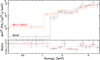 |
Fig. 2. Swift/XRT spectra in 2011–2012 (red) and in 2018 (black), with their best-fit absorbed pexmon model shown as orange and dark gray lines, respectively (top panel) and the data-model ratios (bottom panel). They are corrected for the effective area of the instrument and are given in units of EFE (FE is the energy flux at the energy E). |
The phabs*zphabs*pexmon model is found to reproduce both spectra well (see Fig. 2). By modeling XRT spectra, we confirmed that the intrinsic luminosity (i.e., logL2−10 keV) remains little changed from 2011–2012 to 2018 (see Table 1). In contrast, the intrinsic column density  has significantly increased, from
  cm−2 to
  cm−2. The relatively high
  values support the hypothesis that the source is an absorbed AGN. The observed variation in
  is likely produced by an inner structure around the central black hole, such as the AGN torus.
3. Discussion and conclusion
Because broad Balmer lines are detected in the LIRIS spectrum, we estimated black hole masses with the single-epoch method as follows:
 (1)
(1)
For the case of the Hα line, we adopted a recipe using the Hα-line luminosity (LHα) and its velocity width (FWHMHα) with a = 6.30, b = 0.55, and c = 2.06 provided by Greene & Ho (2005). On the other hand, for the Hβ line, we employed a recipe using the monochromatic continuum luminosity at 5100 Å (L5100) and FWHMHβ with a = 5.36, b = 0.64, and c = 2.00 (Greene & Ho 2005). The estimated black hole mass is log(MBH/M⊙) = 10.9 for both cases (see Table 1). Uncertainties of MBH due to adopting different recipes (e.g., Shen & Liu 2012; Bentz et al. 2013; Jun et al. 2015) are Δ log MBH ∼ 0.3: when we adopt the recent recipes of Jun et al. (2015), for example, black hole masses are derived as log(MBH, Hα/M⊙) = 11.2 and log(MBH, Hβ/M⊙) = 10.8. We also calculated the averaged Eddington ratio of Hα- and Hβ-based black hole masses, that is, log(Lbol, 5100/LEdd)=−0.323, by estimating the AGN bolometric luminosity from the 5100 Å luminosity with a bolometric correction factor of 9.26 (Richards et al. 2006): when we use the 2−10 keV intrinsic X-ray luminosity with the conversion factor given by Marconi et al. (2004), the bolometric luminosity and Eddington ratio are logLbol, X = 48.76 and log(Lbol, X/LEdd) = 0.34, respectively, which is higher than the optical estimates (see Table 1). As described in Sect. 2.2, we detected significant blueshifted outflow components of the [O III]λ4959,5007 lines. This indicates that this DOG is in the blow-out phase at the end of the rapidly obscured black hole growth. This is consistent with Toba et al. (2017b), who indicated that the [O III]λ4959,5007 velocity offset of most DOGs is larger than those of Seyfert 2 galaxies.
In order to derive host-galaxy properties such as stellar mass and IR luminosity of WISE J1042+1641, we carried out the SED fitting with the code investigating galaxy emission (CIGALE; Burgarella et al. 2005; Noll et al. 2009), which enables a SED modeling in a self-consistent manner by taking into account the energy equilibrium between the absorbed energy emitted in the UV/optical from SF/AGN and the re-emitted energy in IR from dust. The SED fitting with CIGALE requires many parameters about the star formation history (SFH), single stellar population (SSP), attenuation law, AGN emission, and dust emission. We applied a “delayed” SFH model that is defined as SFR (t) ∝ t × e−t/τ, where t is the time and τ is the e-folding time of the old stellar population (see, e.g., Ciesla et al. 2016). The age of oldest stars in the galaxy was parameterized with a range of 2.5–12.0 Gyr while the e-folding time was constrained in the range of 250–8000 Myr. For the SSP and attenuation law, we adopted the stellar templates of Bruzual & Charlot (2003) with the Calzetti et al. (2000) dust extinction law assuming a Chabrier (2003) initial mass function (IMF). We also added the standard default nebular emission model included in CIGALE. We assumed solar metallicity (Z = 0.02) for the SSP model, and for the dust attenuation, the color excess of the stellar continuum, E(B−V), was constrained within the range of 0.1–2.0. We used the AGN model provided by Fritz et al. (2006) for the AGN emission (see Ciesla et al. 2015; Toba et al. 2018b, for more detail). For the dust emission, we used the dust model of Draine & Li (2007). The fitting parameters were chosen based on our experiences of SED fitting for DOGs, some of which have a similar optical/IR color as WISE J1042+1641 (e.g., Toba & Nagao 2016; Toba et al. 2017a, 2018b). Therefore, our method with CIGALE is applicable to this object. Under the above configuration with CIGALE, the possible fitting range of stellar mass in this SED fit is 8.72 < log(M⋆/M⊙)< 14.02, which is a sufficiently wide range. In this fitting, we considered SDSS (u′, g′, r′, i′, z′), 2MASS (J, H, Ks), WISE (3.4, 4.6, 12, 22 μm), and AKARI (90 μm) data. We confirmed that WISE J1042+1641 is unresolved at all bands used in this work, which is reasonable because the angular resolutions of the SDSS, 2MASS, and WISE are higher than the size of a lensed system (see the next paragraph). This means that the measured flux density at any band traces the total flux density of the lensed system. The fitting results are shown in Fig. 3.
 |
Fig. 3. SED fitting of WISE J1042+1641. Filled circles represent the observational data from the SDSS (black), 2MASS (red), and WISE (green). The 5σ upper limit from AKARI is denoted as a blue arrow. The best-fit SED is denoted with the black solid line. Different components are also shown: unattenuated stellar emission (green line), attenuated stellar emission (red line), nebular emission (pink line), SF-heated dust emission (light blue line), and AGN emission (blue line). |
We obtained the stellar mass (M⋆) and IR luminosity (LIR), listed in Table 1: the star formation rate was not determined due to the lack of constraints from the far-infrared data. As shown in the table, an extremely high IR luminosity of log(LIR/L⊙) = 14.57, satisfying the criterion for extremely luminous IR galaxies (ELIRGs), and a stellar mass of log(M⋆/M⊙) = 13.55 were obtained. In particular, this stellar mass seems to deviate from the known masses of log(M⋆/M⊙) < 12 (e.g., Gültekin et al. 2009). Moreover, we checked its probability distribution function (PDF) by searching for a secondary peak, which we failed to find, however. This implies that the stellar mass is uniquely determined. Very recently, based on high-resolution J- and H-band (F125W and F160W) imaging data obtained with the Wide Field Camera 3 (WFC3) on the Hubble Space Telescope, Glikman et al. (2018) reported that this object is an anomalous gravitationally lensed quasar, accompanied by four faint (∼5–10% respective fluxes of WISE J1042+1641) sources in the neighborhood (within ∼1.6″), which looks like a quadruply lensed system. They derived its lensing magnification factor of μ = 53−122: the magnification-corrected parameters of black hole mass, stellar mass, and various luminosities are listed in Table 1. In this work, we discuss only the ratio of the black hole to galaxy mass, which is less strongly affected by the magnification correction, instead of absolute values of luminosities and masses. We assumed the same magnification factor for AGN and stellar emission (see also Rusu et al. 2016; Peng et al. 2006b). Although the compact AGN component could be more highly magnified than the host, this would not drastically change our considerations.
In Fig. 4 we plot the ratio of the black hole to galaxy mass of WISE J1042+1641. We adopted the two magnification factors of μ = 53 and 122 that were estimated in Glikman et al. (2018). We expect that the stellar mass at z ∼ 2 and the bulge mass at z = 0 are comparable since WISE J1042+1641, the star-forming galaxy with log(MBH/M⊙)∼10 at z ∼ 2, is likely the progenitor of local bulge-dominated galaxies (e.g., Béthermin et al. 2014). As shown in the figure, we found that the ratio of the black hole to galaxy mass of WISE 1042+1641 (i.e., 0.0083–0.0120) is significantly higher than the ratio in the local Universe, which is log(MBH/M⋆) ∼ 0.001–0.002 (e.g., Marconi & Hunt 2003; Kormendy & Ho 2013). Unless the difference in magnification factors between AGN and host components (i.e., μAGN/μ⋆) is larger than about eight, the MBH/M⋆ ratio lies above the local relation. Our data points follow the sequence of unobscured AGNs (e.g., McLure et al. 2006; Peng et al. 2006b; Targett et al. 2012), which are represented with a gray line, instead of SMGs (Borys et al. 2005; Alexander et al. 2008), which are shown as squares. This result suggests that WISE J1042+1641 is in a blow-out phase at the end of the buried rapid black hole growth, by considering its high Eddington ratios, [O III]λ4959,5007 outflow components, and the moderately high column density derived from X-ray spectra. This is consistent with the recent result by Wu et al. (2018), who suggested that a population of hyperluminous dusty galaxies, the so-called hot DOGs, represents a transitional high-accretion phase between obscured and unobscured quasars (see also Assef et al. 2015). Furthermore, the black hole mass of WISE J1042+1641 is quite high, even assuming the high magnification factor of μ = 122: in this case, we obtain logMBH, Hα = 9.77 with the recipe reported in Greene & Ho (2005). Given the high black hole mass, this object should be the progenitor of a local massive galaxy that evolves to reach the massive end of the sequence of X-ray selected unobscured AGNs, like the source CID-947 studied by Trakhtenbrot et al. (2015), which is shown as a green circle and line in Fig. 4. However, to discuss the obscured evolution of the ratios of black hole to galaxy masses in detail, additional data sets of dusty obscured populations are needed.
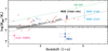 |
Fig. 4. Ratio of black hole to galaxy mass as a function of redshift. The MBH/M⋆ ratios of WISE J1042+1641 are shown as double circles and are color-coded according to the magnification factors of μ = 53 (red) and 122 (blue). The black solid line indicates the MBH/M⋆ sequence of radio-loud AGNs in McLure et al. (2006), followed by unobscured AGNs shown as red and blue open circles for lensed and non-lensed objects, respectively (Peng et al. 2006b). The blue and pink filled squares denote X-ray obscured SMGs and local ULIRGs, respectively (Alexander et al. 2008). SDSS luminous quasars at z ∼ 4 (i.e., SDSS J1310−0055 and SDSS J1446−0101) in Targett et al. (2012) are denoted with light blue open circles. The green open circle denotes an X-ray selected unobscured AGN at the massive end, CDI-947 (Trakhtenbrot et al. 2015), and the green line is a scaled sequence of McLure et al. (2006) to the source. The gray area is the typical mass ratio in the local Universe (Marconi & Hunt 2003). |
Acknowledgments
We would like to thank the anonymous referee for the useful comments and suggestions. We are also grateful to Masamune Oguri, Yuichi Higuchi, Cristian E. Rusu, and Eilat Glikman for helpful comments and suggestions. We thank the WHT staff, especially Ovidiu Vaduvescu and Raine Karjalainen, for invaluable support for the observation. We also thank the Swift operation team for carrying out the X-ray observations. The data analyses were in part carried out on the common-use data analysis computer system at the Astronomy Data Center, ADC, of the National Astronomical Observatory of Japan (NAOJ). K. Matsuoka is supported by Japan Society for the Promotion of Science (JSPS) Overseas Research Fellowships. This work is also supported by JSPS KAKENHI Grant Nos. 18J01050 (Y. Toba), 16H01101, 16H03958, 17H01114 (T. Nagao), 16K17672 (M. Shidatsu), 17K05384 (Y. Ueda), 15H02070, 16K05296 (Y. Terashima), 15K05030 (M. Imanishi). Moreover, Y. Toba and W.-H. Wang acknowledge the support from the Ministry of Science and Technology of Taiwan (MOST 105-2112-M-001-029-MY3). K. Iwasawa acknowledges support by the Spanish MINECO under grant AYA2016-76012-C3-1-P and MDM-2014-0369 of ICCUB (Unidad de Excelencia “María de Maeztu”).
References
- Adelberger, K. L., & Steidel, C. C. 2005, ApJ, 627, L1 [NASA ADS] [CrossRef] [Google Scholar]
- Alexander, D. M., & Hickox, R. C. 2012, New Astron. Rev., 56, 93 [NASA ADS] [CrossRef] [Google Scholar]
- Alexander, D. M., Brandt, W. N., Smail, I., et al. 2008, AJ, 135, 1968 [NASA ADS] [CrossRef] [Google Scholar]
- Assef, R. J., Eisenhardt, P. R. M., Stern, D., et al. 2015, ApJ, 804, 27 [NASA ADS] [CrossRef] [Google Scholar]
- Bentz, M. C., Denney, K. D., Grier, C. J., et al. 2013, ApJ, 767, 149 [NASA ADS] [CrossRef] [Google Scholar]
- Béthermin, M., Kilbinger, M., Daddi, E., et al. 2014, A&A, 567, A103 [NASA ADS] [CrossRef] [EDP Sciences] [Google Scholar]
- Bongiorno, A., Maiolino, R., Brusa, M., et al. 2014, MNRAS, 443, 2077 [NASA ADS] [CrossRef] [Google Scholar]
- Borys, C., Smail, I., Chapman, S. C., et al. 2005, ApJ, 635, 853 [NASA ADS] [CrossRef] [Google Scholar]
- Bruzual, G., & Charlot, S. 2003, MNRAS, 344, 1000 [NASA ADS] [CrossRef] [Google Scholar]
- Burgarella, D., Buat, V., & Iglesias-Páramo, J. 2005, MNRAS, 360, 1413 [NASA ADS] [CrossRef] [Google Scholar]
- Burrows, D. N., Hill, J. E., Nousek, J. A., et al. 2000, Proc. SPIE, 4140, 64 [NASA ADS] [CrossRef] [Google Scholar]
- Calzetti, D., Armus, L., Bohlin, R. C., et al. 2000, ApJ, 533, 682 [NASA ADS] [CrossRef] [Google Scholar]
- Chabrier, G. 2003, PASP, 115, 763 [NASA ADS] [CrossRef] [Google Scholar]
- Ciesla, L., Charmandaris, V., Georgakakis, A., et al. 2015, A&A, 576, A10 [NASA ADS] [CrossRef] [EDP Sciences] [Google Scholar]
- Ciesla, L., Boselli, A., Elbaz, D., et al. 2016, A&A, 585, A43 [NASA ADS] [CrossRef] [EDP Sciences] [Google Scholar]
- Decarli, R., Walter, F., Venemans, B. P., et al. 2018, ApJ, 854, 97 [NASA ADS] [CrossRef] [Google Scholar]
- Dey, A., Soifer, B. T., Desai, V., et al. 2008, ApJ, 677, 943 [NASA ADS] [CrossRef] [Google Scholar]
- Draine, B. T., & Li, A. 2007, ApJ, 657, 810 [NASA ADS] [CrossRef] [Google Scholar]
- Fritz, J., Franceschini, A., & Hatziminaoglou, E. 2006, MNRAS, 366, 767 [Google Scholar]
- Glikman, E., Rusu, C. E., Djorgovski, S. G., et al. 2018, ApJ, submitted [arXiv:1807.05434] [Google Scholar]
- Greene, J. E., & Ho, L. C. 2005, ApJ, 630, 122 [NASA ADS] [CrossRef] [Google Scholar]
- Gültekin, K., Richstone, D. O., Gebhardt, K., et al. 2009, ApJ, 698, 198 [NASA ADS] [CrossRef] [Google Scholar]
- Inada, N., Oguri, M., Pindor, B., et al. 2003, Nature, 426, 810 [NASA ADS] [CrossRef] [PubMed] [Google Scholar]
- Jun, H. D., Im, M., Lee, H. M., et al. 2015, ApJ, 806, 109 [NASA ADS] [CrossRef] [Google Scholar]
- Kalberla, P. M. W., Burton, W. B., Hartmann, D., et al. 2005, A&A, 440, 775 [NASA ADS] [CrossRef] [EDP Sciences] [Google Scholar]
- Kawamuro, T., Ueda, Y., Tazaki, F., Ricci, C., & Terashima, Y. 2016, ApJS, 225, 14 [NASA ADS] [CrossRef] [Google Scholar]
- Kneib, J.-P., Alloin, D., Mellier, Y., et al. 1998, A&A, 329, 827 [NASA ADS] [Google Scholar]
- Kormendy, J., & Ho, L. C. 2013, ARA&A, 51, 511 [Google Scholar]
- Kormendy, J., & Richstone, D. 1995, ARA&A, 33, 581 [NASA ADS] [CrossRef] [Google Scholar]
- Lemon, C. A., Auger, M. W., McMahon, R. G., & Ostrovski, F. 2018, MNRAS, 479, 5060 [NASA ADS] [CrossRef] [Google Scholar]
- Magorrian, J., Tremaine, S., Richstone, D., et al. 1998, AJ, 115, 2285 [NASA ADS] [CrossRef] [Google Scholar]
- Manchado, A., Fuentes, F. J., Prada, F., et al. 1998, Proc. SPIE, 3354, 448 [NASA ADS] [CrossRef] [Google Scholar]
- Marconi, A., & Hunt, L. K. 2003, ApJ, 589, L21 [NASA ADS] [CrossRef] [Google Scholar]
- Marconi, A., Risaliti, G., Gilli, R., et al. 2004, MNRAS, 351, 169 [NASA ADS] [CrossRef] [Google Scholar]
- Matsuoka, K., Silverman, J. D., Schramm, M., et al. 2013, ApJ, 771, 64 [NASA ADS] [CrossRef] [Google Scholar]
- McLure, R. J., Jarvis, M. J., Targett, T. A., Dunlop, J. S., & Best, P. N. 2006, MNRAS, 368, 1395 [NASA ADS] [CrossRef] [Google Scholar]
- Merloni, A., Bongiorno, A., Bolzonella, M., et al. 2010, ApJ, 708, 137 [NASA ADS] [CrossRef] [Google Scholar]
- Morton, D. C. 1991, ApJS, 77, 119 [NASA ADS] [CrossRef] [Google Scholar]
- Nandra, K., O’Neill, P. M., George, I. M., & Reeves, J. N. 2007, MNRAS, 382, 194 [NASA ADS] [CrossRef] [Google Scholar]
- Noll, S., Burgarella, D., Giovannoli, E., et al. 2009, A&A, 507, 1793 [NASA ADS] [CrossRef] [EDP Sciences] [Google Scholar]
- Peng, C. Y., Impey, C. D., Ho, L. C., Barton, E. J., & Rix, H.-W. 2006a, ApJ, 640, 114 [NASA ADS] [CrossRef] [Google Scholar]
- Peng, C. Y., Impey, C. D., Rix, H.-W., et al. 2006b, ApJ, 649, 616 [Google Scholar]
- Richards, G. T., Lacy, M., Storrie-Lombardi, L. J., et al. 2006, ApJS, 166, 470 [NASA ADS] [CrossRef] [Google Scholar]
- Rusu, C. E., Oguri, M., Minowa, Y., et al. 2016, MNRAS, 458, 2 [NASA ADS] [CrossRef] [Google Scholar]
- Sanders, D. B., Soifer, B. T., Elias, J. H., et al. 1988, ApJ, 325, 74 [NASA ADS] [CrossRef] [Google Scholar]
- Schlafly, E. F., & Finkbeiner, D. P. 2011, ApJ, 737, 103 [NASA ADS] [CrossRef] [Google Scholar]
- Schramm, M., & Silverman, J. D. 2013, ApJ, 767, 13 [NASA ADS] [CrossRef] [Google Scholar]
- Shen, Y., & Liu, X. 2012, ApJ, 753, 125 [NASA ADS] [CrossRef] [Google Scholar]
- Shields, G. A., Gebhardt, K., Salviander, S., et al. 2003, ApJ, 583, 124 [NASA ADS] [CrossRef] [Google Scholar]
- Skrutskie, M. F., Cutri, R. M., Stiening, R., et al. 2006, AJ, 131, 1163 [NASA ADS] [CrossRef] [Google Scholar]
- Targett, T. A., Dunlop, J. S., & McLure, R. J. 2012, MNRAS, 420, 3621 [NASA ADS] [CrossRef] [Google Scholar]
- Toba, Y., & Nagao, T. 2016, ApJ, 820, 46 [NASA ADS] [CrossRef] [Google Scholar]
- Toba, Y., Nagao, T., Strauss, M. A., et al. 2015, PASJ, 67, 86 [NASA ADS] [CrossRef] [Google Scholar]
- Toba, Y., Nagao, T., Wang, W.-H., et al. 2017a, ApJ, 840, 21 [NASA ADS] [CrossRef] [Google Scholar]
- Toba, Y., Bae, H.-J., Nagao, T., et al. 2017b, ApJ, 850, 140 [NASA ADS] [CrossRef] [Google Scholar]
- Toba, Y., Ueda, J., Lim, C.-F., et al. 2018a, ApJ, 857, 31 [NASA ADS] [CrossRef] [Google Scholar]
- Toba, Y., Ueda, Y., Matsuoka, K., et al. 2018b, MNRAS, submitted [Google Scholar]
- Trakhtenbrot, B., Urry, C. M., Civano, F., et al. 2015, Science, 349, 168 [NASA ADS] [CrossRef] [Google Scholar]
- Ueda, Y., Hatsukade, B., Kohno, K., et al. 2018, ApJ, 853, 24 [NASA ADS] [CrossRef] [Google Scholar]
- Véron-Cetty, M.-P., Joly, M., & Véron, P. 2004, A&A, 417, 515 [NASA ADS] [CrossRef] [EDP Sciences] [Google Scholar]
- Woo, J.-H., Treu, T., Malkan, M. A., & Blandford, R. D. 2008, ApJ, 681, 925 [NASA ADS] [CrossRef] [Google Scholar]
- Woo, J.-H., Schulze, A., Park, D., et al. 2013, ApJ, 772, 49 [NASA ADS] [CrossRef] [Google Scholar]
- Wright, E. L., Eisenhardt, P. R. M., Mainzer, A. K., et al. 2010, AJ, 140, 1868 [NASA ADS] [CrossRef] [Google Scholar]
- Wu, J., Jun, H. D., Assef, R. J., et al. 2018, ApJ, 852, 96 [NASA ADS] [CrossRef] [Google Scholar]
- Wyithe, J. S. B., & Loeb, A. 2003, ApJ, 595, 614 [NASA ADS] [CrossRef] [Google Scholar]
- York, D. G., Adelman, J., Anderson, Jr., J. E., et al. 2000, AJ, 120, 1579 [CrossRef] [Google Scholar]
All Tables
All Figures
|
Fig. 1. Final reduced spectrum of WISE J1042+1641 observed with LIRIS shown as the black line. Red vertical lines indicate the central wavelengths of rest-frame optical emission lines, i.e., Hγ, Hβ, [O III]λ4959, [O III]λ5007, [N II]λ6548, Hα, and [N II]λ6583. The best-fit model for the observed spectrum is indicated as the red line, and the residual is shown as a dark gray line. The continuum (green line) and individual emission-line components (blue lines) are also shown. The gray shaded area was excluded in the fit. The small inset panel shows the same spectrum zoomed in to focus on the blueshifted outflow components in oxygen lines: blueshifted and unshifted lines are indicated as purple and orange lines, respectively. |
| In the text | |
|
Fig. 2. Swift/XRT spectra in 2011–2012 (red) and in 2018 (black), with their best-fit absorbed pexmon model shown as orange and dark gray lines, respectively (top panel) and the data-model ratios (bottom panel). They are corrected for the effective area of the instrument and are given in units of EFE (FE is the energy flux at the energy E). |
| In the text | |
|
Fig. 3. SED fitting of WISE J1042+1641. Filled circles represent the observational data from the SDSS (black), 2MASS (red), and WISE (green). The 5σ upper limit from AKARI is denoted as a blue arrow. The best-fit SED is denoted with the black solid line. Different components are also shown: unattenuated stellar emission (green line), attenuated stellar emission (red line), nebular emission (pink line), SF-heated dust emission (light blue line), and AGN emission (blue line). |
| In the text | |
|
Fig. 4. Ratio of black hole to galaxy mass as a function of redshift. The MBH/M⋆ ratios of WISE J1042+1641 are shown as double circles and are color-coded according to the magnification factors of μ = 53 (red) and 122 (blue). The black solid line indicates the MBH/M⋆ sequence of radio-loud AGNs in McLure et al. (2006), followed by unobscured AGNs shown as red and blue open circles for lensed and non-lensed objects, respectively (Peng et al. 2006b). The blue and pink filled squares denote X-ray obscured SMGs and local ULIRGs, respectively (Alexander et al. 2008). SDSS luminous quasars at z ∼ 4 (i.e., SDSS J1310−0055 and SDSS J1446−0101) in Targett et al. (2012) are denoted with light blue open circles. The green open circle denotes an X-ray selected unobscured AGN at the massive end, CDI-947 (Trakhtenbrot et al. 2015), and the green line is a scaled sequence of McLure et al. (2006) to the source. The gray area is the typical mass ratio in the local Universe (Marconi & Hunt 2003). |
| In the text | |
Current usage metrics show cumulative count of Article Views (full-text article views including HTML views, PDF and ePub downloads, according to the available data) and Abstracts Views on Vision4Press platform.
Data correspond to usage on the plateform after 2015. The current usage metrics is available 48-96 hours after online publication and is updated daily on week days.
Initial download of the metrics may take a while.