© ESO 2018

1. Introduction

Local helioseismology aims at studying the solar interior in three dimensions by exploiting the information contained in the waves observed at the solar surface (see, e.g., Gizon & Birch 2005 and references therein). Helioseismic holography is one particular approach of local helioseismology, which images subsurface scatterers by back-propagating the surface wave field to target points in the interior. Helioseismic holography is also known as Lindsey-Braun (LB) holography (Lindsey & Braun 1997, 2000a and references therein). It has been used to study solar convection (Braun et al. 2004, 2007), active region emergence (Birch et al. 2013, 2016), sunspot subsurface structure (Braun & Birch 2008b; Birch et al. 2009), to image wave sources (Lindsey et al. 2006), to study sunquakes caused by solar flares (Zharkov et al. 2013; Besliu-Ionescu et al. 2017), and to detect active regions on the far side of the Sun (Lindsey & Braun 2000b; Liewer et al. 2014).

In acoustics, a well-established version of holography in a medium that contains sources is Porter-Bojarski (PB) holography (Porter & Devaney 1982). PB holography uses both the wave field and its normal derivative at the surface to produce holographic images (Porter 1969). PB holography was introduced in helioseismology by Skartlien (2001, 2002), where deterministic sources and scatterers were recovered in a solar background. Yang (2018) recently studied PB holographic images in a homogeneous medium permeated by localized deterministic sources to study ghost images near the observational boundary.

In this paper we apply PB holography in a realistic helioseismological setting. First we rewrote the wave equation in Helmholtz form, in order to properly define the Green’s functions that are involved in the definition of PB holographic data. The background density and sound-speed are taken from a standard solar model. The model of wave excitation is described by a reasonable source covariance function, which leads to a solar-like power spectrum for acoustic oscillations.

The signal is defined as the expectation value of the holographic image intensity that results from perturbations in sound speed, density, and flows with respect to the reference solar model. The corresponding sensitivity kernels were computed in the first-order Born approximation (Gizon & Birch 2002; Birch & Gizon 2007; Braun et al. 2007; Birch et al. 2011). This signal must take into account the correlations between incident and scattered wave fields, which are both connected to the sources of excitation (turbulent convection).

Random noise in holographic images is due to the stochastic nature of the sources of excitation. While noise can sometimes be estimated from the data (Lindsey & Braun 1990; Braun & Birch 2008a), a theoretical understanding is useful to design holographic experiments. In this paper we have extended the noise model developed in time-distance helioseismology to holography (Gizon & Birch 2004; Fournier et al. 2014). We did not attempt to image individual sources as in Skartlien (2002), which in our view is not a well-posed problem (see also Lindsey et al. 2006), except in the case of sunquakes. Instead we considered sources to be specified through a source covariance function.

2. Reduced wave equation

At angular frequency ω and spatial position r in the computational domain V, the propagation of acoustic waves in a 3D heterogeneous moving medium is described by the displacement vector ξ(r, ω), solution to

$$\begin{array}{c}\hfill -{(\omega +\mathrm{i}\gamma +\mathrm{i}\mathit{u}·\mathrm{\nabla })}^2\mathit{\xi }-\frac{1}{\rho }\mathrm{\nabla }(\rho c^2\mathrm{\nabla }·\mathit{\xi })+\text{gravity terms}=\mathit{F},\end{array}$$(1)

where ρ(r) and c(r) are the density and sound speed, and u(r) is a steady vector flow. Wave attenuation is included through the function γ(r, ω). The source term F(r, ω) is a realization from a random process; it describes the stochastic excitation of the waves by turbulent convection. Following Lamb (1909) and Deubner & Gough (1984), we consider the scalar variable

$$\begin{array}{c}\hfill \psi ={\rho }^{1/2}{c}^2\mathrm{\nabla }·\mathit{\xi }\end{array}$$(2)

to recast the wave equation into a Helmholtz-like equation

$$\begin{array}{c}\hfill L\psi :=-(\mathrm{\Delta }+k^2)\psi -\frac{2\mathrm{i}\omega }{{\rho }^{1/2}c}\rho \mathit{u}·\mathrm{\nabla }\left(\frac{\psi }{{\rho }^{1/2}c}\right)=S,\end{array}$$(3)

where S = ρ^1/2c²∇⋅F is a scalar source term. The local wavenumber k(r, ω) is given by

$$\begin{array}{c}\hfill k^2=\frac{({\omega }^2+2\mathrm{i}\omega \gamma )-{\omega }_{\mathrm{c}}^2}{c^2},\end{array}$$(4)

where the squared acoustic cut-off frequency is

$$\begin{array}{c}\hfill {\omega }_{\mathrm{c}}^2={\rho }^{1/2}{c}^2\mathrm{\Delta }({\rho }^{-1/2}).\end{array}$$(5)

In obtaining Eq. (3), we ignored gravity terms and assumed slow variations of c, u, and γ compared to the wavelength (Gizon et al. 2017). The advection term is such that the corresponding operator is Hermitian symmetric for the inner product $\langle {\psi }_1,{\psi }_2\rangle ={\displaystyle \int {\psi }_1^{*}}{\psi }_2\text{d}V$ under the conditions that the flow conserves mass and that it does not cross the boundary (u_n = 0 on ∂V).

The stochastic sources of excitation are assumed to be stationary and spatially uncorrelated. They are described by a source covariance function of the form

$$\begin{array}{c}\hfill \mathbb{E}[S^{\ast }(\mathit{r},\omega )S({\mathit{r}}^{\prime },\omega )]=M(\mathit{r},\omega )\delta (\mathit{r}-{\mathit{r}}^{\prime }).\end{array}$$(6)

To solve Eq. (3), one needs to specify a boundary condition at the computational boundary. Here we apply an outgoing radiation boundary condition

$$\begin{array}{c}\hfill {\partial }_n\psi =\mathrm{i}{k}_n\psi \text{on}\partial V.\end{array}$$(7)

We applied the boundary condition (Atmo RBC 1) from Barucq et al. (2018), which assumes an exponential decay of the background density at the boundary of the domain but neglects curvature. Then, the local wavenumber k_n from Eq. (7) is given by

$$\begin{array}{c}\hfill k_n^2=\frac{{\omega }^2+2\mathrm{i}\omega \gamma }{c^2}-\frac{1}{4H^2},\end{array}$$(8)

where H = −1/(d ln ρ/dr) is the density scale height at the boundary. The last term in Eq. (8) is connected to the cut-off frequency for an isothermal atmosphere (Lamb 1909), thus k_n is an approximation of the wavenumber k from Eq. (4). Fournier et al. (2017) discuss several of the boundary conditions derived in Barucq et al. (2018).

3. Holographic image intensity

The following calculations are done at constant ω, thus we drop ω from the list of function arguments when not explicitly needed. The Porter–Bojarski integral is defined by Porter & Devaney (1982):

$$\begin{array}{c}\hfill {\mathrm{\Phi }}_{\alpha }(\mathit{x},A):={\displaystyle {\int }_A[\psi (\mathit{r}){\partial }_n{H}_{\alpha }(\mathit{r},\mathit{x})-H_{\alpha }(\mathit{r},\mathit{x}){\partial }_n\psi (\mathit{r})]\mathrm{d}\mathit{r},}\end{array}$$(9)

where H_α is an acoustic wave propagator for the reference medium and A is a surface on the Sun where ψ and ∂_nψ are observed. The role of H_α is to propagate the wave field backward (or forward) in time, which leads to the concept of egression (or ingression) in LB holography (Lindsey & Braun 2000a).

Several choices for the propagators have been proposed in the literature, as detailed in Table 1. These depend on the outgoing (G₀) and incoming ($G_0^{-}$) Green’s functions defined in a reference medium with ρ₀, c₀, γ₀, and u₀ = 0:

$$\begin{array}{ccc}\hfill L_0[G_0(\mathit{r},{\mathit{r}}^{\prime })]=\delta (\mathit{r}-{\mathit{r}}^{\prime })& \text{and}\hfill & \hfill {\partial }_n{G}_0=\mathrm{i}{k}_n{G}_0\text{on}\partial V,\end{array}$$(10)

$$\begin{array}{ccc}\hfill L_0[G_0^{-}(\mathit{r},{\mathit{r}}^{\prime })]=\delta (\mathit{r}-{\mathit{r}}^{\prime })& \text{and}\hfill & \hfill {\partial }_n{G}_0^{-}=-\mathrm{i}{k}_n{G}_0^{-}\text{on}\partial V,\end{array}$$(11)

with

$$\begin{array}{c}\hfill L_0=-(\mathrm{\Delta }+k_0^2),\end{array}$$(12)

where k₀ is k in the reference medium and k_n is from Eq. (8). The Green’s functions $G_0^{\ast }$ or $G_0^{-}$ are backward propagators (cf. egression), while (${(G_0^{-})}^{\ast }$ is a forward propagator (cf. ingression). When the surface A is closed, it is equivalent to use $G_0^{\ast }$ and Im G₀ (Devaney & Porter 1985). Tsang et al. (1987) proposed $H_{\alpha }=G_0^{-}$ as a backward propagator to correct for wave attenuation.

If the observations are made at the computational boundary and the wave field satisfies the same boundary condition as the Green’s function, then Eq. (9) reads

$$\begin{array}{c}\hfill {\mathrm{\Phi }}_{\alpha }(\mathit{x},A)={\displaystyle {\int }_A\psi (\mathit{r})[{\partial }_n{H}_{\alpha }(\mathit{r},\mathit{x})-\mathrm{i}{k}_n{H}_{\alpha }(\mathit{r},\mathit{x})]\mathrm{d}\mathit{r}.}\end{array}$$(13)

When $H_{\alpha }=G_0^{\ast }$, we have

$$\begin{array}{c}\hfill \mathrm{\Phi }(\mathit{x},A)=-2\mathrm{i}\text{Re}[k_n]{\displaystyle {\int }_A\psi (\mathit{r})G_0^{\ast }(\mathit{r},\mathit{x})\mathrm{d}\mathit{r},}\end{array}$$(14)

which corresponds to the egression as defined by Lindsey & Braun (2000a). Thus LB and PB integrals are closely related, at least for the upper boundary condition employed here.

In LB holography, information is extracted from the egression-ingression correlation (wave-speed perturbations and flows) and from the egression power (source covariance). Analogously, we define the PB image intensity (or covariance) as

$$\begin{array}{c}\hfill I_{\alpha \beta }(\mathit{x},A,A^{\prime })={\mathrm{\Phi }}_{\alpha }^{\ast }(\mathit{x},A){\mathrm{\Phi }}_{\beta }(\mathit{x},A^{\prime }).\end{array}$$(15)

For the case α = β we define

$$\begin{array}{c}\hfill I_{\alpha }(\mathit{x},A)={|{\mathrm{\Phi }}_{\alpha }^{\ast }(\mathit{x},A)|}^2.\end{array}$$(16)

Different choices of pupils and propagators will provide sensitivity to different quantities as shown in Table 2. Scatterers are detected by correlating the forward and backward propagated wavefields. Different pupil shapes give access to different components of the flow (Table 2 and Fig. 1).

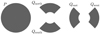Fig. 1. Pupil geometries used to compute sound-speed or source kernels (P) and flow kernels (Qs), also see Table 2.

4. First-order perturbations with respect to a reference solar model

We wish to study how perturbations to the background medium affect the holographic images. Using the Born approximation, the first step is to express the perturbations to the wavefield and use this expression in Eq. (9) to obtain the perturbations to the PB integral and the image intensity.

4.1. Perturbations to the wavefield

We considered perturbations δc, δρ, δγ, u with respect to the reference medium defined by ρ₀, c₀, γ₀, and u₀ = 0. The perturbations to the sources of excitation are described through the perturbations to the source covariance,

$$\begin{array}{c}\hfill M(\mathit{r},\omega )=M_0(\mathit{r},\omega )+\delta M(\mathit{r},\omega ),\end{array}$$(17)

where

$$\begin{array}{c}\hfill \delta M(\mathit{r},\omega )=\mathbb{E}[S_0^{\ast }(\mathit{r})\delta S({\mathit{r}}^{\prime })+\delta S^{\ast }(\mathit{r})S_0({\mathit{r}}^{\prime })]=ϵ(\mathit{r})M_0(\mathit{r},\omega ).\end{array}$$(18)

Using the Born approximation up to first order, we write the wave field as

$$\begin{array}{c}\hfill \psi (\mathit{r},\omega )={\psi }_0(\mathit{r},\omega )+\delta \psi (\mathit{r},\omega ),\end{array}$$(19)

where the zeroth- and first-order wave fields are given by

$$\begin{array}{cc}\hfill L_0[{\psi }_0]& \hfill =S_0,\hfill \end{array}$$(20)

$$\begin{array}{cc}\hfill L_0[\delta \psi ]& \hfill =-\delta L[{\psi }_0]+\delta S.\hfill \end{array}$$(21)

The perturbed wave operator is

$$\begin{array}{c}\hfill \delta L[{\psi }_0]=-\delta k^2{\psi }_0-\frac{2\mathrm{i}\omega }{{\rho }_0^{1/2}{c}_0}{\rho }_0\mathit{u}·\mathrm{\nabla }\left(\frac{{\psi }_0}{{\rho }_0^{1/2}{c}_0}\right),\end{array}$$(22)

with

$$\begin{array}{c}\hfill c_0^2\delta k^2=2\mathrm{i}\omega \delta \gamma -({\omega }^2+2\mathrm{i}\omega {\gamma }_0)\frac{\delta c^2}{c_0^2}-{\left(\frac{\partial {\omega }_{\mathrm{c}}^2}{\partial \rho }\right)}_0\delta \rho .\end{array}$$(23)

In terms of the Green’s function G₀, we have

$$\begin{array}{cc}& \hfill \psi (\mathit{r})={\psi }_0(\mathit{r})+{\displaystyle {\int }_V{G}_0(\mathit{r},{\mathit{r}}_{\mathrm{s}})\delta k^2({\mathit{r}}_{\mathrm{s}}){\psi }_0({\mathit{r}}_{\mathrm{s}})\mathrm{d}{\mathit{r}}_{\mathrm{s}}+{\int }_V{G}_0(\mathit{r},\mathit{s})\delta S(\mathit{s})\mathrm{d}\mathit{s}}\hfill \\ \hfill & \hfill +2\mathrm{i}\omega {\displaystyle {\int }_V{\rho }_0({\mathit{r}}_{\mathrm{s}}){\mathit{u}}_0({\mathit{r}}_{\mathrm{s}})·\mathrm{\nabla }\left(\frac{G_0(\mathit{r},{\mathit{r}}_{\mathrm{s}})}{{\rho }_0^{1/2}({\mathit{r}}_{\mathrm{s}})c_0({\mathit{r}}_{\mathrm{s}})}\right)\frac{{\psi }_0({\mathit{r}}_{\mathrm{s}})}{{\rho }_0^{1/2}({\mathit{r}}_{\mathrm{s}})c_0({\mathit{r}}_{\mathrm{s}})}\mathrm{d}{\mathit{r}}_{\mathrm{s}}.}\hfill \end{array}$$(24)

where the scattering location r_​s spans the entire solar volume V.

4.2. Perturbations to the PB integral

For convenience, we introduce the source kernels

$$\begin{array}{c}\hfill K_{\alpha }(\mathit{x},\mathit{s},A)={\displaystyle {\int }_A[G(\mathit{r},\mathit{s}){\partial }_n{H}_{\alpha }(\mathit{r},\mathit{x})-H_{\alpha }(\mathit{r},\mathit{x}){\partial }_{n}G(\mathit{r},\mathit{s})]\mathrm{d}\mathit{r},}\end{array}$$(25)

such that the PB integral is given by

$$\begin{array}{c}\hfill {\mathrm{\Phi }}_{\alpha }(\mathit{x},A)={\displaystyle {\int }_V{K}_{\alpha }(\mathit{x},\mathit{s},A)S(\mathit{s})\mathrm{d}\mathit{s}.}\end{array}$$(26)

We denote by K_α, 0 the source kernel in the reference medium (when G is replaced by G₀).

Replacing the wavefield by its first order expansion (Eq. (24)) in the definition of the PB integral (Eq. (9)), one obtains

$$\begin{array}{c}\hfill {\mathrm{\Phi }}_{\alpha }(\mathit{x},A)={\mathrm{\Phi }}_{\alpha ,0}(\mathit{x},A)+\delta {\mathrm{\Phi }}_{\alpha }(\mathit{x},A),\end{array}$$(27)

where Φ_α, 0 is the value for the reference medium and δΦ_α is due to perturbations in the medium:

$$\begin{array}{c}\hfill \delta {\mathrm{\Phi }}_{\alpha }(\mathit{x},A)={\displaystyle {\int }_V\delta K_{\alpha }(\mathit{x},\mathit{s},A)S(\mathit{s})\mathrm{d}\mathit{s}+{\int }_V{K}_{\alpha ,0}(\mathit{x},\mathit{s},A)\delta S(\mathit{s})\mathrm{d}\mathit{s},}\end{array}$$(28)

where

$$\begin{array}{cc}\hfill \delta K_{\alpha }& \hfill (\mathit{x},\mathit{s},A)={\displaystyle {\int }_V{K}_{\alpha ,0}(\mathit{x},{\mathit{r}}_{\mathrm{s}},A)\delta k^2({\mathit{r}}_{\mathrm{s}})G_0({\mathit{r}}_{\mathrm{s}},\mathit{s})\mathrm{d}{\mathit{r}}_{\mathrm{s}}}\hfill \\ \hfill & \hfill +2\mathrm{i}\omega {\displaystyle {\int }_V\frac{K_{\alpha ,0}(\mathit{x},{\mathit{r}}_{\mathrm{s}},A)}{{\rho }_0^{1/2}({\mathit{r}}_{\mathrm{s}})c_0({\mathit{r}}_{\mathrm{s}})}{\rho }_0{\mathit{u}}_0·\mathrm{\nabla }\left(\frac{G_0({\mathit{r}}_{\mathrm{s}},\mathit{s})}{{\rho }_0^{1/2}({\mathit{r}}_{\mathrm{s}})c_0({\mathit{r}}_{\mathrm{s}})}\right)\mathrm{d}{\mathit{r}}_{\mathrm{s}}.}\hfill \end{array}$$(29)

4.3. Perturbations to the image intensity

We write the holographic image intensity to first order in the form

$$\begin{array}{c}\hfill I_{\alpha \beta }(\mathit{x},A,A^{\prime })=I_{\alpha \beta ,0}(\mathit{x},A,A^{\prime })+{\delta I}_{\alpha \beta }(\mathit{x},A,A^{\prime }).\end{array}$$(30)

The expectation values of the zeroth- and first-order image intensities are

$$\begin{array}{cc}\hfill \mathbb{E}[I_{\alpha \beta ,0}(\mathit{x},A,A^{\prime })]& \hfill ={\displaystyle {\int }_V{K}_{\alpha ,0}^{\ast }(\mathit{x},\mathit{s},A)K_{\beta ,0}(\mathit{x},\mathit{s},A^{\prime })M_0(\mathit{s})\mathrm{d}\mathit{s},}\hfill \end{array}$$(31)

$$\begin{array}{cc}\hfill \mathbb{E}[{\delta I}_{\alpha \beta }(\mathit{x},A,A^{\prime })]& \hfill ={\displaystyle {\int }_V{K}_{\alpha ,0}^{\ast }(\mathit{x},\mathit{s},A){\delta K}_{\beta }(\mathit{x},\mathit{s},A^{\prime })M_0(\mathit{s})\mathrm{d}\mathit{s}}\hfill \\ \hfill & \hfill +{\displaystyle {\int }_V{\delta K}_{\alpha }^{\ast }(\mathit{x},\mathit{s},A)K_{\beta ,0}(\mathit{x},\mathit{s},A^{\prime })M_0(\mathit{s})\mathrm{d}\mathit{s}}\hfill \\ \hfill & \hfill +{\displaystyle {\int }_V{K}_{\alpha ,0}^{\ast }(\mathit{x},\mathit{s},A)K_{\beta ,0}(\mathit{x},\mathit{s},A^{\prime })ϵ(\mathit{s})M_0(\mathit{s})\mathrm{d}\mathit{s}.}\hfill \end{array}$$(32)

Using the definition of the source kernels, we obtain

$$\begin{array}{c}\hfill \mathbb{E}[I_{\alpha \beta ,0}(\mathit{x},A,A^{\prime })]={⟨⟨C_0(\mathit{r},{\mathit{r}}^{\prime })⟩⟩}_{\alpha \beta }(\mathit{x},A,A^{\prime }),\end{array}$$(33)

where

$$\begin{array}{c}\hfill C_0(\mathit{r},{\mathit{r}}^{\prime })={\displaystyle {\int }_V{G}_0^{\ast }(\mathit{r},\mathit{s})G_0({\mathit{r}}^{\prime },\mathit{s})M_0(\mathit{s})\mathrm{d}\mathit{s}}\end{array}$$(34)

is the expectation value of the cross-covariance function and, for any function F(r, r′), the double brackets mean

$$\begin{array}{cc}\hfill {⟨⟨F(\mathit{r},{\mathit{r}}^{\prime })⟩⟩}_{\alpha \beta }(\mathit{x},A,A^{\prime })& \hfill =\hfill \\ \hfill {\displaystyle {\int }_A\mathrm{d}\mathit{r}{\int }_{A^{\prime }}\mathrm{d}{\mathit{r}}^{\prime }[}& \hfill {\partial }_n{H}_{\alpha }^{\ast }(\mathit{r},\mathit{x})F(\mathit{r},{\mathit{r}}^{\prime }){\partial }_{n^{\prime }}{H}_{\beta }({\mathit{r}}^{\prime },\mathit{x})\hfill \\ \hfill & \hfill -H_{\alpha }^{\ast }(\mathit{r},\mathit{x}){\partial }_{n}F(\mathit{r},{\mathit{r}}^{\prime }){\partial }_{n^{\prime }}{H}_{\beta }({\mathit{r}}^{\prime },\mathit{x})\hfill \\ \hfill & \hfill -{\partial }_n{H}_{\alpha }^{\ast }(\mathit{r},\mathit{x}){\partial }_{n}F(\mathit{r},{\mathit{r}}^{\prime })H_{\beta }({\mathit{r}}^{\prime },\mathit{x})\hfill \\ \hfill & \hfill +H_{\alpha }^{\ast }(\mathit{r},\mathit{x}){\partial }_n{\partial }_{n^{\prime }}F(\mathit{r},{\mathit{r}}^{\prime })H_{\beta }({\mathit{r}}^{\prime },\mathit{x})].\hfill \end{array}$$(35)

The perturbation to the image intensity is given by

$$\begin{array}{cc}& \hfill \mathbb{E}[{\delta I}_{\alpha \beta }(\mathit{x},A,A^{\prime })]\hfill \\ \hfill & \hfill ={\displaystyle {\int }_Vϵ(\mathit{s}){\mathcal{K}}_{\alpha \beta }^{ϵ}(\mathit{x},\mathit{s},A,A^{\prime })\mathrm{d}\mathit{s}}\hfill \\ \hfill & \hfill +{\displaystyle {\int }_V(\delta k^{2\ast }({\mathit{r}}_{\mathrm{s}}){\mathcal{K}}_{\alpha \beta }^k(\mathit{x},{\mathit{r}}_{\mathrm{s}},A,A^{\prime })+\delta k^2({\mathit{r}}_{\mathrm{s}}){\mathcal{K}}_{\beta \alpha }^{k\ast }(\mathit{x},{\mathit{r}}_{\mathrm{s}},A^{\prime },A))\mathrm{d}{\mathit{r}}_{\mathrm{s}}}\hfill \\ \hfill & \hfill +2\mathrm{i}\omega {\displaystyle {\int }_V\mathit{u}({\mathit{r}}_{\mathrm{s}})·({\mathcal{K}}_{\alpha \beta }^u(\mathit{x},{\mathit{r}}_{\mathrm{s}},A,A^{\prime })-{\mathcal{K}}_{\beta \alpha }^{u\ast }(\mathit{x},{\mathit{r}}_{\mathrm{s}},A^{\prime },A))\mathrm{d}{\mathit{r}}_{\mathrm{s}},}\hfill \end{array}$$(36)

where

$$\begin{array}{cc}\hfill {\mathcal{K}}_{\alpha \beta }^{ϵ}& \hfill (\mathit{x},\mathit{s},A,A^{\prime })=M_0(\mathit{s}){\langle \langle G_0^{\ast }(\mathit{r},\mathit{s})G_0({\mathit{r}}^{\prime },\mathit{s})\rangle \rangle }_{\alpha \beta }(\mathit{x},A,A^{\prime }),\hfill \end{array}$$(37)

$$\begin{array}{cc}\hfill {\mathcal{K}}_{\alpha \beta }^k& \hfill (\mathit{x},{\mathit{r}}_{\mathrm{s}},A,A^{\prime })={\langle \langle C_0({\mathit{r}}_{\mathrm{s}},{\mathit{r}}^{\prime })G_0^{\ast }(\mathit{r},{\mathit{r}}_{\mathrm{s}})\rangle \rangle }_{\alpha \beta }(\mathit{x},A,A^{\prime }),\hfill \end{array}$$(38)

$$\begin{array}{cc}\hfill {\mathcal{K}}_{\alpha \beta }^u& \hfill (\mathit{x},{\mathit{r}}_{\mathrm{s}},A,A^{\prime })=\hfill \\ \hfill & \hfill {\displaystyle {\langle \langle \mathrm{\nabla }\left(\frac{C_0({\mathit{r}}_{\mathrm{s}},{\mathit{r}}^{\prime })}{{\rho }_0{({\mathit{r}}_{\mathrm{s}})}^{1/2}{c}_0({\mathit{r}}_{\mathrm{s}})}\right)\frac{{\rho }_0{({\mathit{r}}_{\mathrm{s}})}^{1/2}{G}_0^{\ast }(\mathit{r},{\mathit{r}}_{\mathrm{s}})}{c_0({\mathit{r}}_{\mathrm{s}})}\rangle \rangle }_{\alpha \beta }(\mathit{x},A,A^{\prime }).}\hfill \end{array}$$(39)

The kernels for δk² and δk^2* can be combined using Eq. (23) to obtain kernels for sound-speed ${\mathcal{K}}_{\alpha \beta }^c$, density ${\mathcal{K}}_{\alpha \beta }^{\rho }$ and attenuation ${\mathcal{K}}_{\alpha \beta }^{\gamma }$. For example,

$$\begin{array}{c}\hfill \mathbb{E}[{\delta I}_{\alpha \beta }(\mathit{x},A,A^{\prime })]={\displaystyle {\int }_V\delta c({\mathit{r}}_{\mathrm{s}}){\mathcal{K}}_{\alpha \beta }^c(\mathit{x},{\mathit{r}}_{\mathrm{s}},A,A^{\prime })\mathrm{d}{\mathit{r}}_{\mathrm{s}}}\end{array}$$(40)

with

$$\begin{array}{cc}\hfill {\mathcal{K}}_{\alpha \beta }^c(\mathit{x},{\mathit{r}}_{\mathrm{s}},A,A^{\prime })=& \hfill -\frac{2({\omega }^2-2\mathrm{i}\omega \gamma )}{c_0^3({\mathit{r}}_{\mathrm{s}})}{\mathcal{K}}_{\alpha \beta }^k(\mathit{x},{\mathit{r}}_{\mathrm{s}},A,A^{\prime })\hfill \\ \hfill & \hfill -\frac{2({\omega }^2+2\mathrm{i}\omega \gamma )}{c_0^3({\mathit{r}}_{\mathrm{s}})}{\mathcal{K}}_{\beta \alpha }^{k\ast }(\mathit{x},{\mathit{r}}_{\mathrm{s}},A^{\prime },A).\hfill \end{array}$$(41)

4.4. Choice of the source covariance

In order to compute the above kernels, we still need to choose the source covariance function M₀ in order to define the reference cross-covariance C₀ using Eq. (34). One possibility is to place the sources at a single depth, a few hundred kilometers below the solar surface.

Another possibility is to choose a source covariance of the form

$$\begin{array}{c}\hfill M_0(\mathit{r},\omega )=\mathrm{\Pi }(\omega )\frac{\gamma (\mathit{r},\omega )}{c_0^2(\mathit{r})},\end{array}$$(42)

where Π(ω) is the source power spectrum (see Gizon et al. 2017). This choice implies

$$\begin{array}{c}\hfill C_0(\mathit{r},{\mathit{r}}^{\prime },\omega )=\frac{\mathrm{\Pi }(\omega )}{2\omega }\mathrm{Im}{G}_0({\mathit{r}}^{\prime },\mathit{r},\omega )+\text{surface term}.\end{array}$$(43)

The surface term depends on the boundary condition. It vanishes for a Dirichlet boundary condition (free surface), while it remains for radiative boundary conditions (e.g., Sommerfeld). Below the acoustic cutoff frequency, modes are trapped well below the observational and computational boundaries and the surface term is negligible. In this paper we use Eq. (42) in the convection zone and switch off the sources above the photosphere. By doing so, the surface term in Eq. (43) vanishes.

5. Noise

To compute the noise level, we computed the variance of the image intensity in the absence of scatterers:

$$\begin{array}{cc}\hfill \mathrm{Var}[I_{\alpha \beta ,0}(\mathit{x})]& \hfill =\mathrm{Var}\left[{\displaystyle \int K_{\alpha ,0}^{\ast }(\mathit{x},\mathit{s})K_{\beta ,0}(\mathit{x},{\mathit{s}}^{\prime })S^{\ast }(\mathit{s})S({\mathit{s}}^{\prime })\mathrm{d}\mathit{s}\mathrm{d}{\mathit{s}}^{\prime }}\right]\hfill \\ \hfill & \hfill ={\displaystyle {\int }_{V^4}{K}_{\alpha ,0}^{\ast }(\mathit{x},{\mathit{s}}_1)K_{\beta ,0}(\mathit{x},{\mathit{s}}_1^{\prime })K_{\alpha ,0}(\mathit{x},{\mathit{s}}_2)K_{\beta ,0}^{\ast }(\mathit{x},{\mathit{s}}_2^{\prime })}\hfill \\ \hfill & \hfill \times M_4({\mathit{s}}_1,{\mathit{s}}_1^{\prime },{\mathit{s}}_2,{\mathit{s}}_2^{\prime })\mathrm{d}{\mathit{s}}_1\mathrm{d}{\mathit{s}}_1^{\prime }\mathrm{d}{\mathit{s}}_2\mathrm{d}{\mathit{s}}_2^{\prime }\hfill \\ \hfill & \hfill -{\left|{\displaystyle {\int }_{V^2}{K}_{\alpha ,0}^{\ast }(\mathit{x},\mathit{s})K_{\beta ,0}(\mathit{x},{\mathit{s}}^{\prime })\mathbb{E}\left[S^{\ast }(\mathit{s})S({\mathit{s}}^{\prime })\right]\mathrm{d}\mathit{s}\mathrm{d}{\mathit{s}}^{\prime }}\right|}^2,\hfill \end{array}$$(44)

where

$$\begin{array}{c}\hfill M_4({\mathit{s}}_1,{\mathit{s}}_1^{\prime },{\mathit{s}}_2,{\mathit{s}}_2^{\prime })=\mathbb{E}\left[S^{\ast }({\mathit{s}}_1)S({\mathit{s}}_1^{\prime })S({\mathit{s}}_2)S^{\ast }({\mathit{s}}_2^{\prime })\right].\end{array}$$(45)

Under the (very reasonable) assumption that S is a realization drawn from a Gaussian random process, the fourth-order moment is the sum of products of the second-order moments:

$$\begin{array}{cc}& \hfill M_4({\mathit{s}}_1,{\mathit{s}}_1^{\prime },{\mathit{s}}_2,{\mathit{s}}_2^{\prime })=\mathbb{E}\left[S^{\ast }({\mathit{s}}_1)S({\mathit{s}}_1^{\prime })\right]\mathbb{E}\left[S({\mathit{s}}_2)S^{\ast }({\mathit{s}}_2^{\prime })\right]\hfill \\ \hfill & \hfill +\mathbb{E}\left[S^{\ast }({\mathit{s}}_1)S({\mathit{s}}_2)\right]\mathbb{E}\left[S({\mathit{s}}_1^{\prime })S^{\ast }({\mathit{s}}_2^{\prime })\right]\hfill \\ \hfill & \hfill +\mathbb{E}\left[S^{\ast }({\mathit{s}}_1)S^{\ast }({\mathit{s}}_2^{\prime })\right]\mathbb{E}\left[S({\mathit{s}}_2)S({\mathit{s}}_1^{\prime })\right].\hfill \end{array}$$(46)

The first term in M₄ cancels out the squared term in Eq. (44). The third term is zero as the frequencies are uncorrelated. Thus,

$$\begin{array}{cc}\hfill \mathrm{Var}[I_{\alpha \beta ,0}(\mathit{x})]& \hfill ={\displaystyle {\int }_{V^4}{K}_{\alpha ,0}^{\ast }(\mathit{x},{\mathit{s}}_1)K_{\beta ,0}(\mathit{x},{\mathit{s}}_1^{\prime })K_{\alpha ,0}(\mathit{x},{\mathit{s}}_2)K_{\beta ,0}^{\ast }(\mathit{x},{\mathit{s}}_2^{\prime })}\hfill \\ \hfill & \hfill \times \mathbb{E}\left[S^{\ast }({\mathit{s}}_1)S({\mathit{s}}_2)\right]\mathbb{E}\left[S({\mathit{s}}_1^{\prime })S^{\ast }({\mathit{s}}_2^{\prime })\right]\mathrm{d}{\mathit{s}}_1\mathrm{d}{\mathit{s}}_1^{\prime }\mathrm{d}{\mathit{s}}_2\mathrm{d}{\mathit{s}}_2^{\prime }\hfill \\ \hfill & \hfill ={\displaystyle {\int }_V|K_{\alpha ,0}{(\mathit{x},\mathit{s})|}^{2}M(\mathit{s})\mathrm{d}\mathit{s}{\int }_V{|K_{\beta ,0}(\mathit{x},\mathit{s})|}^{2}M(\mathit{s})\mathrm{d}\mathit{s}}\hfill \\ \hfill & \hfill =\mathbb{E}[I_{\alpha ,0}(\mathit{x})]\mathbb{E}[I_{\beta ,0}(\mathit{x})].\hfill \end{array}$$(47)

When α = β, the standard deviation of I_α, 0 is equal to its expectation value. This is because the probability density function of I_α, 0 is a χ² with two degrees of freedom, in other words, an exponential distribution.

6. Average over frequencies

In order to increase the signal-to-noise ratio (S/N), one usually averages the image intensity over a range of frequencies [ω₀ − Δω/2, ω₀ + Δω/2]. For an observation duration T, this interval will contain N = Δω T/2π independent frequencies.

The frequency-averaged perturbation to the image intensity (i.e. the signal) is denoted by

$$\begin{array}{c}\hfill ⟨{\delta I}_{\alpha \beta }(\mathit{x})⟩=\frac{1}{N}{\displaystyle \sum _{i=1}^N}{\delta I}_{\alpha \beta }(\mathit{x},{\omega }_i).\end{array}$$(48)

The variance of the noise in the average image intensity is then given by

$$\begin{array}{cc}\hfill \mathrm{Var}\langle I_{\alpha \beta ,0}(\mathit{x})\rangle & \hfill =\mathrm{Var}\left(\frac{1}{N}{\displaystyle \sum _{i=1}^N}{I}_{\alpha \beta ,0}(\mathit{x},{\omega }_i)\right)\hfill \end{array}$$(49)

$$\begin{array}{cc}& \hfill =\frac{1}{N^2}{\displaystyle \sum _{i=1}^N}\mathrm{Var}{I}_{\alpha \beta ,0}(\mathit{x},{\omega }_i)\hfill \end{array}$$(50)

$$\begin{array}{cc}& \hfill =\frac{1}{N}\langle \mathrm{Var}{I}_{\alpha \beta ,0}(\mathit{x})\rangle ,\hfill \end{array}$$(51)

since the noise in the data at different frequencies is uncorrelated.

The expected S/N is thus

$$\begin{array}{c}\hfill \mathrm{SNR}(\mathit{x})=\frac{|\mathbb{E}⟨{\delta I}_{\alpha \beta }(\mathit{x})⟩|}{\sqrt{\mathrm{Var}⟨I_{\alpha \beta ,0}(\mathit{x})⟩}}=\frac{\sqrt{N}|\mathbb{E}⟨{\delta I}_{\alpha \beta }(\mathit{x})⟩|}{\sqrt{⟨\mathbb{E}[I_{\alpha ,0}(\mathit{x})]\mathbb{E}[I_{\beta ,0}(\mathit{x})]⟩}}·\end{array}$$(52)

The number of available frequencies N within a fixed frequency band Δω is proportional to the observation duration T, hence the noise level goes like T^−1/2. Provided that the frequency interval Δω is small with respect to the variations of the signal, then the S/N will increase as T^1/2.

7. Example computations

In order to illustrate the theory, we have computed holographic images in the presence of sound-speed perturbations at different depths and calculate the corresponding S/Ns.

7.1. Reference Green’s function

The main input quantity required to compute PB integrals is the reference Green’s function (Eq. (10)). Here it is computed in the frequency domain using the spherically-symmetric standard solar Model S (Christensen-Dalsgaard et al. 1996). The wave attenuation model is taken from Gizon et al. (2017). Below 5.3 mHz, we have γ = γ₀|ω/ω₀|^5.77, where γ₀/2π = 4.29 μHz and ω₀/2π = 3 mHz. Above 5.3 mHz, γ/2π = 125 μHz is kept constant. The radiation boundary condition defined by Eq. (7) is applied at the computational boundary located 500 km above the solar surface with the local wavenumber k_n (where H = 105 km). The wave equation is solved using the finite-element solver Montjoie (Duruflé 2006; Gizon et al. 2017).

The reference Green’s function only depends on the angular distance Θ between the two points at radii r and r′. To speed up the computations, we place one of the points on the polar axis and compute the axisymmetric component of the Green’s function $G_l^{m=0}(r,r\prime ,\omega )$ at each spherical harmonic degree l, to obtain:

$$\begin{array}{c}\hfill G_0(\mathit{r},{\mathit{r}}^{\prime },\omega )\simeq {\displaystyle \sum _{l=0}^{l_{\max }}}{G}_l^{m=0}(r,r^{\prime },\omega )P_l(cos\mathrm{\Theta }),\end{array}$$(53)

where we used an approximate equality because the sum is truncated at l_max = 300.

7.2. Sound-speed kernels

The sound-speed kernel is computed using Eq. (41) and the definition of ${\mathcal{K}}_{\alpha \beta }^k$. We need to evaluate two surface integrals, which can be computed analytically via a decomposition of all quantities into spherical harmonic coefficients (Fournier et al. 2018).

Figure 2 shows a sound-speed kernel ${\mathcal{K}}_{\alpha \beta }^c$ at a single frequency of 3 mHz. The pupil P is a polar cap of angular size 120° and the wave propagators H_α and H_β are given in Table 2. As expected the kernel peaks around the scatterer position at z = 0.7 R_⊙. A cut along the polar axis is shown in Fig. 3; the kernel width is about half the local wavelength. In addition, we find ghost values at the antipode.

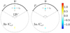Fig. 2. Meridional slice through the sound-speed kernel ${\mathcal{K}}_{\alpha \beta }^c$(x, r​s) computed in Model S at a single frequency of 3 mHz, in units of 10−34 kg m−3 s−3. Both the real (left panel) and imaginary (right panel) parts of the kernel are shown. The scatterer at zs = 0.7 R⊙ is indicated by the crosses. The observation pupil P is a polar cap of full angular size 120°. We notice the “ghost values” at the antipode.

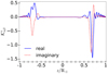Fig. 3. Cut along the z axis through the sound-speed kernel from Fig. 2. The scatterer is at zs = 0.7 R⊙.

7.3. Signal

At position ${\mathit{r}}_{\mathrm{s}}=z_{\mathrm{s}}\widehat{\mathbf{z}}$ along the polar axis, we consider a localized increase in sound speed of 10% over a volume V_s, such that the signal (Eq. (40)) may be written as

$$\begin{array}{c}\hfill \mathbb{E}[{\delta I}_{\alpha \beta }(\mathit{x})]\simeq 0.1V_{\mathrm{s}}{c}_0({\mathit{r}}_{\mathrm{s}}){\mathcal{K}}_{\alpha \beta }^c(\mathit{x},{\mathit{r}}_{\mathrm{s}}).\end{array}$$(54)

The volume V_s is that of a ball of diameter λ(r_s)/2 = π/[Re k(r_s, ω₀)] with ω₀/2π = 3 mHz. This is an approximate but much faster way to compute the effect of a perturbation of volume comparable to the highest possible holographic resolution. We checked that the answer does not differ significantly from the one obtained by integrating numerically the kernel over the ball of volume V_s. For reference, we note that λ/2 = 38 Mm at r = 0.7 R_⊙ and λ/2 = 20 Mm at r = 0.9 R_⊙.

Figure 4 shows the signal |𝔼[δI_αβ(x)]| for sound-speed perturbations located at two different depths z_s = 0.7 R_⊙ (red curve) and 0.9 R_⊙ (blue curve). The pupil P and the wave propagators are the same as those of Fig. 2. The left panel of Fig. 4 shows the results at a single frequency of 3 mHz. With only one frequency, the signal peaks close to the scattering location but the spatial resolution is relatively poor, with a ghost on the far side. To demonstrate the benefits of averaging, the right panel shows the signal after averaging over 101 frequencies uniformly distributed in the interval 2.75–3.25 mHz. The frequency resolution 5 μHz corresponds to an observation duration T = 55.5 h. Averaging over frequencies improves the spatial resolution which approaches λ/2 and the ghost is suppressed. A horizontal line segment is plotted on the right panel at each depth to mark half the local wavelength.

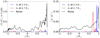Fig. 4. Left panel: image intensity |𝔼[δIαβ(x)]| at a single frequency of 3 mHz, as a function of position x along the z-axis. The sound-speed perturbation (see Eq. (54)) is placed at two different positions along the z-axis, zs = 0.7 R⊙ (red) and 0.9 R⊙ (blue). The standard deviation of the noise $\sqrt{\mathrm{Var}⟨I_{\alpha \beta ,0}(\mathit{x})⟩}$ is given by the black curve. We note that the jagged aspect of the curves is not due to numerical inaccuracies. Right panel: Image intensity and noise level after averaging over 101 frequencies uniformly distributed in the interval from 2.75 to 3.25 mHz. The frequency resolution is 5 μHz, implying an observation duration of T = 55.5 h. A horizontal line segment is plotted at each depth to mark half of the local wavelength.

As seen in Fig. 5 the spatial extent of the frequency-averaged kernels is approximately λ/2 in both the radial and horizontal directions, for all scattering points in the range 0.6 <  z_s/R_⊙ <  0.98. Thus helioseismic holography is a diffraction-limited imaging technique as suggested by Lindsey & Braun (1997).

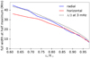Fig. 5. Radial and horizontal widths of the frequency-averaged sound-speed kernel |⟨𝒦c⟩| as functions of scattering position. These are close to half the local wavelength at 3 mHz (dotted line).

7.4. Noise

The noise is obtained from Eq. (47), which requires the computation of 𝔼[I_α, 0] and 𝔼[I_β, 0] using Eq. (33). The reference cross-covariance C₀ is precomputed. The double surface integral is evaluated in a similar way as for the kernel computations.

For a frequency of 3 mHz the left panel of Fig. 4 (black curve) shows the noise level, together with the signal described in the previous section. The jagged aspect of the noise variations with position is not due to numerical inaccuracies but to the details of the Green’s function. As shown in the right panel of Fig. 4, the noise level goes down by a factor of about ten after averaging over 101 frequencies, and varies more smoothly with depth.

Braun & Birch (2008a) studied the noise level in observed travel times measured from LB holography. These measurements, however, include contributions from supergranulation and so are not directly comparable to what is shown in Fig. 4.

7.5. Signal-to-noise ratio

Figure 6 shows the S/N as a function of scatterer location. We recall that the sound-speed perturbation is specified by Eq. (54) and is the same as in Sect. 7.3. The results are shown at a single frequency of 3 mHz and after averaging over 101 frequencies in the interval 2.75–3.25 mHz. After averaging, the S/N is above two and is roughly independent of depth in the range 0.6 <  z_s/R_⊙ <  0.98 for a pupil of angular size 120°. We note that the ghost at −z_s is much below the noise level.

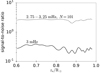Fig. 6. S/N in PB image intensity for a 10% sound-speed perturbation over a volume Vs(zs) placed at zs along the polar axis (Eq. (54)). The results are shown at a single frequency of 3 mHz (solid curve) and after averaging over 101 frequencies in the interval from 2.75 to 3.25 mHz (dashed curve).

We find that both signal and noise vary rapidly with frequency for deep located sound-speed scatterers. Figure 7 shows an example of a sound-speed scatterer located at z_s = 0.7 R_⊙. Strong frequency variations in signal and noise are evident for frequencies below 3.5 mHz. This can be understood as follows. Low-frequency modes have narrowly-peaked power spectra due to their long lifetimes. At these low frequencies, the amplitude of the kernel function and the noise will change rapidly when the frequency coincides with a particular mode frequency. Additionally, the kernel function may not peak exactly at the sound-speed scatterer position when only a few modes contribute to the kernel function. Figure 8 shows the S/N as a function of frequency for a sound-speed scatterer located at z_s = 0.9 R_⊙. For this target depth closer to the surface, the rapid variations disappear above 3 mHz, due to the larger contribution of high-degree modes which are not resolved in frequency space because of their short lifetimes.

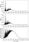Fig. 7. Signal, noise, and S/N as function of frequency for a sound-speed scatterer located at zs = 0.7 R⊙. Here we show the result for a frequency range of 2–7 mHz. The rapid changes are not due to numerical inaccuracies. The red dots indicate the values at frequency 2.4000 mHz.

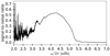Fig. 8. S/N as in Fig. 7, but for a sound-speed scatterer located closer to the surface at zs = 0.9 R⊙.

The kernel function at frequency 2.4000 mHz for z_s = 0.7 R_⊙ is shown in Fig. 9; this particular frequency corresponds to the peak indicated in Fig. 7 with a red dot. We see that this kernel is much less localized around the scattering point than the kernel at 3 mHz (Fig. 2).

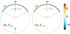Fig. 9. Meridional slice of the sound-speed kernel ${\mathcal{K}}_{\alpha \beta }^c$ with zs = 0.7 R⊙ computed at the low frequency of 2.4000 mHz, which corresponds to the spike with a red dot in Fig. 7. This kernel displays oscillations and is not peaked as much as the 3 mHz kernel from Fig. 2.

8. Conclusion

We derived a framework for computing the expected signal and the noise level in PB helioseismic holography. The same framework could be used to interpret LB data, including phase-sensitive data.

Porter-Bojarski holography requires knowledge of the wave field, ψ = ρ^1/2c²∇⋅ξ, and its normal derivative on the solar surface, ∂_nψ. With this definition of ψ, the Green’s function used in the definition of PB integrals solves a well-defined Helmholtz-like equation, which we solve numerically (Gizon et al. 2017). The need for finite-frequency Green’s functions was demonstrated in LB holography by Pérez Hernández & González Hernández (2010). In the numerical examples shown in the previous section, we assumed that we have full knowledge of ∂_nψ on the surface. In practice, we do not observe directly the normal derivative of the wave field; it must be approximated. According to complementary simulations (not shown here), this can be achieved by using the approximate outgoing radiation condition ∂_nψ = ik_nψ derived by Barucq et al. (2018).

We found that, for a sufficiently large pupil, scatterers can be imaged at a resolution that is very close to half the local wavelength, λ/2. This confirms the claim by Lindsey & Braun (1997, 2000a) that helioseismic holography is diffraction-limited. In that sense, helioseismic holography is superior to deep-focusing time-distance helioseismology, which gives lower spatial resolution (Munk 2001; Pourabdian et al. 2018). For large pupils, we found that the S/N in PB images does not vary much with depth in the convection zone, when a perturbation in sound-speed fills a volume corresponding to the holographic resolution.

Averaging over frequencies improves the S/N. For a scatterer at the bottom of the convection zone, the signal and the noise vary smoothly with frequency above 4 mHz (see Fig. 7). At lower frequencies, however, the signal varies rapidly with frequency (due to contributions from individual long-lived p modes) and it is not obvious how the signal should be averaged. A specific analysis of low-frequency data is required, especially for deep scatterers.

We found that the S/N in PB holography is maximum around 3.7 mHz for z_s = 0.7 R_⊙ (resp. at 4.3 mHz for z_s = 0.9 R_⊙). There is no indication in our calculations that there is a benefit in using the frequencies above the acoustic cutoff (unlike predictions by Ruzmaikin & Lindsey 2003). The S/N drops to very small values above 5 mHz. One may ask if this drop is somehow compensated by the increase in spatial resolution at high frequencies. The answer is negative. Our calculations indicate that noise has a horizontal correlation length that is about half the local wavelength. Far too few independent measurements are available at high frequencies to recover an acceptable S/N by horizontal spatial averaging.

Our synthetic data do not contain a convective background. The effect of this background on S/Ns in holography should be studied. Future work should also investigate the performance of PB holography for target locations that are away from the axis of the pupil, especially for farside imaging applications.

Acknowledgments

The theoretical framework was developed by L.G. and D.F. at Mathematisches Forchungsinstitut Oberwolfach in May 2017. The numerical computations were performed by D.Y. using the Montjoie solver. D.Y. is a member of the International Max Planck Research School for Solar System Science at the University of Göttingen. We thank M. Duruflé and J. Chabassier from Inria Magique-3D for the helioseismology-related developments of Montjoie. We also thank Chris Hanson from NYUAD for the fine tuning of the model power spectrum of solar oscillations. L.G. acknowledges support from NYUAD Institute grant G1502. The computing resources were provided in part by the German Data Center for SDO, a project funded by the German Aerospace Center (DLR).

References

All Tables

All Figures

	Fig. 1. Pupil geometries used to compute sound-speed or source kernels (P) and flow kernels (Qs), also see Table 2.
In the text

Fig. 2. Meridional slice through the sound-speed kernel ${\mathcal{K}}_{\alpha \beta }^c$(x, r​s) computed in Model S at a single frequency of 3 mHz, in units of 10−34 kg m−3 s−3. Both the real (left panel) and imaginary (right panel) parts of the kernel are shown. The scatterer at zs = 0.7 R⊙ is indicated by the crosses. The observation pupil P is a polar cap of full angular size 120°. We notice the “ghost values” at the antipode.

In the text

	Fig. 3. Cut along the z axis through the sound-speed kernel from Fig. 2. The scatterer is at zs = 0.7 R⊙.
In the text

Fig. 4. Left panel: image intensity |𝔼[δIαβ(x)]| at a single frequency of 3 mHz, as a function of position x along the z-axis. The sound-speed perturbation (see Eq. (54)) is placed at two different positions along the z-axis, zs = 0.7 R⊙ (red) and 0.9 R⊙ (blue). The standard deviation of the noise $\sqrt{\mathrm{Var}⟨I_{\alpha \beta ,0}(\mathit{x})⟩}$ is given by the black curve. We note that the jagged aspect of the curves is not due to numerical inaccuracies. Right panel: Image intensity and noise level after averaging over 101 frequencies uniformly distributed in the interval from 2.75 to 3.25 mHz. The frequency resolution is 5 μHz, implying an observation duration of T = 55.5 h. A horizontal line segment is plotted at each depth to mark half of the local wavelength.

In the text

	Fig. 5. Radial and horizontal widths of the frequency-averaged sound-speed kernel |⟨𝒦c⟩| as functions of scattering position. These are close to half the local wavelength at 3 mHz (dotted line).
In the text

	Fig. 6. S/N in PB image intensity for a 10% sound-speed perturbation over a volume Vs(zs) placed at zs along the polar axis (Eq. (54)). The results are shown at a single frequency of 3 mHz (solid curve) and after averaging over 101 frequencies in the interval from 2.75 to 3.25 mHz (dashed curve).
In the text

	Fig. 7. Signal, noise, and S/N as function of frequency for a sound-speed scatterer located at zs = 0.7 R⊙. Here we show the result for a frequency range of 2–7 mHz. The rapid changes are not due to numerical inaccuracies. The red dots indicate the values at frequency 2.4000 mHz.
In the text

	Fig. 8. S/N as in Fig. 7, but for a sound-speed scatterer located closer to the surface at zs = 0.9 R⊙.
In the text

	Fig. 9. Meridional slice of the sound-speed kernel ${\mathcal{K}}_{\alpha \beta }^c$ with zs = 0.7 R⊙ computed at the low frequency of 2.4000 mHz, which corresponds to the spike with a red dot in Fig. 7. This kernel displays oscillations and is not peaked as much as the 3 mHz kernel from Fig. 2.
In the text

References

- Barucq, H., Chabassier, J., Duruflé, M., Gizon, L., & Leguèbe, M. 2018, Math. Modell. Numer. Anal., 52, 945 [Google Scholar]
- Besliu-Ionescu, D., Donea, A., & Cally, P. 2017, Sun Geosphere, 12, 59 [NASA ADS] [Google Scholar]
- Birch, A. C., Braun, D. C., Hanasoge, S. M., & Cameron, R. 2009, Sol. Phys., 254, 17 [NASA ADS] [CrossRef] [Google Scholar]
- Birch, A. C., Braun, D. C., Leka, K. D., Barnes, G., & Javornik, B. 2013, ApJ, 762, 131 [NASA ADS] [CrossRef] [Google Scholar]
- Birch, A. C., & Gizon, L. 2007, Astron. Nachr., 328, 228 [NASA ADS] [CrossRef] [Google Scholar]
- Birch, A. C., Parchevsky, K. V., Braun, D. C., & Kosovichev, A. G. 2011, Sol. Phys., 272, 11 [NASA ADS] [CrossRef] [Google Scholar]
- Birch, A. C., Schunker, H., Braun, D. C., et al. 2016, Sci. Adv., 2, e1600557 [NASA ADS] [CrossRef] [Google Scholar]
- Braun, D. C., & Birch, A. C. 2008a, ApJ, 689, L161 [NASA ADS] [CrossRef] [Google Scholar]
- Braun, D. C., & Birch, A. C. 2008b, Sol. Phys., 251, 267 [NASA ADS] [CrossRef] [Google Scholar]
- Braun, D. C., Birch, A. C., & Lindsey, C. 2004, in SOHO 14 Helio- and Asteroseismology: Towards a Golden Future, ed. D. Danesy, ESA SP, 559, 337 [NASA ADS] [Google Scholar]
- Braun, D. C., Birch, A. C., Benson, D., Stein, R. F., & Nordlund, Å. 2007, ApJ, 669, 1395 [NASA ADS] [CrossRef] [Google Scholar]
- Christensen-Dalsgaard, J., Däppen, W., Ajukov, S. V., et al. 1996, Science, 272, 1286 [CrossRef] [Google Scholar]
- Deubner, F.-L., & Gough, D. 1984, ARA&A, 22, 593 [NASA ADS] [CrossRef] [Google Scholar]
- Devaney, A., & Porter, R. 1985, JOSA A, 2, 2006 [NASA ADS] [CrossRef] [Google Scholar]
- Duruflé, M. 2006, PhD Thesis, ENSTA ParisTech, France [Google Scholar]
- Fournier, D., Gizon, L., Hohage, T., & Birch, A. C. 2014, A&A, 567, A137 [NASA ADS] [CrossRef] [EDP Sciences] [Google Scholar]
- Fournier, D., Leguèbe, M., Hanson, C. S., et al. 2017, A&A, 608, A109 [CrossRef] [EDP Sciences] [Google Scholar]
- Fournier, D., Hanson, C. S., Gizon, L., & Barucq, H. 2018, A&A, 616, A156 [NASA ADS] [CrossRef] [EDP Sciences] [Google Scholar]
- Gizon, L., & Birch, A. C. 2002, ApJ, 571, 966 [NASA ADS] [CrossRef] [Google Scholar]
- Gizon, L., & Birch, A. C. 2004, ApJ, 614, 472 [NASA ADS] [CrossRef] [Google Scholar]
- Gizon, L., & Birch, A. C. 2005, Liv. Rev. Sol. Phys., 2, 6 [Google Scholar]
- Gizon, L., Barucq, H., Duruflé, M., et al. 2017, A&A, 600, A35 [NASA ADS] [CrossRef] [EDP Sciences] [Google Scholar]
- Lamb, H. 1909, Proc. London Math. Soc., 7, 122 [Google Scholar]
- Liewer, P. C., González Hernández, I., Hall, J. R., Lindsey, C., & Lin, X. 2014, Sol. Phys., 289, 3617 [Google Scholar]
- Lindsey, C., & Braun, D. C. 1990, Sol. Phys., 126, 101 [Google Scholar]
- Lindsey, C., & Braun, D. C. 1997, ApJ, 485, 895 [Google Scholar]
- Lindsey, C., & Braun, D. C. 2000a, Sol. Phys., 192, 261 [NASA ADS] [CrossRef] [Google Scholar]
- Lindsey, C., & Braun, D. C. 2000b, Science, 287, 1799 [NASA ADS] [CrossRef] [Google Scholar]
- Lindsey, C., Birch, A. C., & Donea, A. C. 2006, in Solar MHD Theory and Observations: A High Spatial Resolution Perspective, eds. J. Leibacher, R. F. Stein, & H. Uitenbroek, ASP Conf. Ser., 354, 174 [NASA ADS] [Google Scholar]
- Munk, J. M. 2001, PhD Thesis, University of Aarhus, Aarhus, Denmark [Google Scholar]
- Pérez Hernández, F., & González Hernández, I. 2010, ApJ, 711, 853 [NASA ADS] [CrossRef] [Google Scholar]
- Porter, R. P. 1969, Phys. Lett. A, 29, 193 [NASA ADS] [CrossRef] [Google Scholar]
- Porter, R. P., & Devaney, A. J. 1982, JOSA, 72, 327 [NASA ADS] [CrossRef] [Google Scholar]
- Pourabdian, M., Fournier, D., & Gizon, L. 2018, Sol. Phys., 293, 66 [NASA ADS] [CrossRef] [Google Scholar]
- Ruzmaikin, A., & Lindsey, C. 2003, in GONG+ 2002. Local and Global Helioseismology: the Present and Future, ed. H. Sawaya-Lacoste, ESA SP, 517, 71 [NASA ADS] [Google Scholar]
- Skartlien, R. 2001, ApJ, 554, 488 [NASA ADS] [CrossRef] [Google Scholar]
- Skartlien, R. 2002, ApJ, 565, 1348 [NASA ADS] [CrossRef] [Google Scholar]
- Tsang, L., Ishimaru, A., Porter, R. P., & Rouseff, D. 1987, JOSA A, 4, 1783 [NASA ADS] [CrossRef] [Google Scholar]
- Yang, D. 2018, Sol. Phys., 293, 17 [NASA ADS] [CrossRef] [Google Scholar]
- Zharkov, S., Green, L. M., Matthews, S. A., & Zharkova, V. V. 2013, Sol. Phys., 284, 315 [NASA ADS] [CrossRef] [Google Scholar]
All Tables
Proposed propagators and associated pupils (Hα, A) and (Hβ, A′) for different types of perturbations.