| Issue |
A&A
Volume 620, December 2018
|
|
|---|---|---|
| Article Number | A42 | |
| Number of page(s) | 10 | |
| Section | Astrophysical processes | |
| DOI | https://doi.org/10.1051/0004-6361/201833506 | |
| Published online | 29 November 2018 | |
Physics of the Applegate mechanism: Eclipsing time variations from magnetic activity
1
Hamburger Sternwarte, Universität Hamburg, Gojenbergsweg 112, 21029 Hamburg, Germany
e-mail: This email address is being protected from spambots. You need JavaScript enabled to view it.
2
Departamento de Astronomía, Facultad Ciencias Físicas y Matemáticas, Universidad de Concepción, Av. Esteban Iturra s/n Barrio Universitario, Casilla 160-C, Concepción, Chile
Received:
26
May
2018
Accepted:
4
September
2018
Abstract
Since its proposal in 1992, the Applegate mechanism has been discussed as a potential intrinsical mechanism to explain transit-timing variations in various types of close binary systems. Most analytical arguments presented so far focused on the energetic feasibility of the mechanism while applying rather crude one- or two-zone prescriptions to describe the exchange of angular momentum within the star. In this paper, we present the most detailed approach to date to describe the physics giving rise to the modulation period from kinetic and magnetic fluctuations. Assuming moderate levels of stellar parameter fluctuations, we find that the resulting binary period variations are one or two orders of magnitude lower than the observed values in RS-CVn like systems, supporting the conclusion of existing theoretical work that the Applegate mechanism may not suffice to produce the observed variations in these systems. The most promising Applegate candidates are low-mass post-common-envelope binaries with binary separations ≲1 R⊙ and secondary masses in the range of 0.30 M⊙ and 0.36 M⊙.
Key words: stars: activity / stars: interiors / stars: AGB and post-AGB / binaries: eclipsing
© ESO 2018
1. Introduction
Precise timing measurements in close binaries routinely reveal variations in the eclipse timings. While for binaries with very short periods of less than three hours gravitational wave emission is the dominating means of angular momentum loss, magnetic braking can account for such effects in binaries with longer periods (see, e.g., Kraft et al. 1962; Faulkner 1971; Verbunt & Zwaan 1981; Parsons et al. 2013). A subclass of close binaries, mainly RS Canum Venaticorum (RS CVn) and post-common envelope binary (PCEB) systems, feature cyclic or nearly-periodic orbital period variations on timescales of a few years to decades that are incompatible with classical gravitational wave or magnetic braking models (see, e.g., Lanza et al. 1998; Brinkworth et al. 2006; Zorotovic & Schreiber 2013). For some systems, planetary companions may explain these variations (see, e.g., Qian et al. 2011; Beuermann et al. 2013; Nasiroglu et al. 2017; Han et al. 2017), while some of the planetary solutions were found to be dynamically unstable (Horner et al. 2013) or have been proven incorrect observationally (Hardy et al. 2015). On the other hand, the period variations in other systems such as QS Vir are still not well understood (Parsons et al. 2010).
Based on and inspired by earlier work by Matese & Whitmire (1983) and Applegate & Patterson (1987), Applegate (1992) proposed a new mechanism to explain cyclic orbital period variations in close binaries. The author assumed a time-dependent gravitational quadrupole moment modulated by the stellar activity cycle. Given a constant orbital angular momentum, an increasing quadrupole moment results in a stronger gravitational field and finally in a decreasing orbital radius and increasing orbital velocity, which can be observed as a reduction of the binary period.
To calculate the required energy as well as the expected quadrupole changes, Applegate (1992) considered a thin shell rotating in a point mass potential representing the rest of the star. The author assumed that the torque necessary to perform the angular momentum exchange is provided by subsurface magnetic fields of a few kG. Given such a field, luminosity variations on the 10% level and angular velocity variations on the 1% level are expected, leading to binary period variations compatible with the observed values in RS CVn systems (ΔP/P ∼ 10−5). Applegate (1992) made a number of testable predictions, which included significant period luminosity changes due to temperature variations and a 1:1 relation between the modulation period and the stellar activity cycle. Both processes have been observed in systems such as CG Cygni, accompanied by orbital period variations (Hall 1991), while luminosity variations can be observed by studying photospheric temperatures (see, e.g., Gray & Baliunas 1994).
Lanza et al. (1998) generalized the magnetohydrodynamic aspects of the pioneering work of Applegate (1992), included the effects of internal magnetic fields, and elaborated on the connection between the Applegate mechanism and different types of dynamo models, emphasizing that a careful study of the Applegate mechanism may allow distinguishing between them. The improved Lanza et al. (1998) model is based on the momentum balance equation and assumes a uniform ratio of plasma pressure to magnetic pressure over the star. Expansion of the gravitational potential in spherical harmonics allowed Lanza et al. (1998) to calculate the quadrupole potential at the surface of the star, finding that the angular velocity changes required to produce a certain amount of period variation are reduced by a factor of 2 compared to the original Applegate (1992) approach.
Furthermore, Lanza et al. (1998) found that the driver of the period variations is the magnetic dynamo of the active component, which can effectively transform kinetic energy from nuclear reactions into magnetic energy and is more likely to be an α2Ω dynamo, introducing a further observational aspect. Lanza & Rodonò (1999) stressed that the original Applegate (1992) ansatz may systematically overestimate the energies required to power the quadrupole moment variations as the exchanges between kinetic and magnetic energy are cyclic and partially reversible processes. Therefore, the authors concluded that the original model only provides upper limits for the required energy.
Lanza (2005) revisited the original work by Applegate (1992) and introduced an entirely new approach. Assuming that the angular velocity of the active component is only a function of the distance from its rotation axis, Lanza (2005) considered angular momentum redistributions not only between two layers, but rather general radial transport and redistribution modes within the convection zone. Imposing a strictly adiabatic convection zone and neglecting density perturbations, the author considered the equations of mass continuity and angular momentum conservation within a mean-field framework. Solving the angular momentum equation, Lanza (2005) calculated individual angular momentum redistribution modes from which he derived both the amplitude of the quadrupole moment change and the kinetic energy dissipated during the redistribution processes. Contrary to prior works, Lanza (2005) found that the power required to drive the observed levels of binary period variation in HR 1099 exceeds the luminosity provided by the active component by one or two orders of magnitude. Lanza (2006) extended the Lanza (2005) approach to angular velocity distributions that are functions of both radius and latitude, finding that the Applegate effect is still not a viable option in the case of HR 1099 and RS CVn systems in general.
Another route has been taken by Brinkworth et al. (2006), who generalized the original Applegate (1992) thin-shell ansatz to angular momentum exchanges between a finite core and a finite shell, including the core back-reaction to oblateness changes of the surrounding shell. Völschow et al. (2016) extended the Brinkworth et al. (2006) model to realistic stellar density profiles, derived analytic expressions to estimate the energy required to produce a certain level of period variation in a given system, and applied their full model to a set of 16 close binary systems, including 11 PCEBs. In line with previous works, the authors found that the Applegate effect cannot uniquely explain period variations in close binaries, and only 4 of the 16 systems were identified as potential Applegate candidates. Most recently, Navarrete et al. (2018) employed the analytic two-zone model by Völschow et al. (2016) to investigate how rotation affects the energetic feasibility of the Applegate effect and on which scale the activity cycle matches the observed modulation period, noting that the systems with the highest rotation rates are the most likely Applegate candidates. However, one critical simplification of both the Brinkworth et al. (2006) and Völschow et al. (2016) models is that the authors set the core-shell transition where it minimizes the energy necessary to power the Applegate effect.
In this paper, we extend the Lanza (2006) model by assuming a time-dependent magnetic field, velocity field fluctuations, and magnetic field fluctuations in the convection zone from which we can explicitly calculate the temporal evolution of the dissipated energy as well as the binary period variation. In addition, we consider superpositions of angular momentum redistribution modes instead of calculating the quadrupole moment changes caused by individual modes, as previously done by Lanza (2005, 2006). For the sake of consistency, we first apply our model to HR 1099 and use the system as an illustrative example for the basic predictions we make, before we extend our analysis to PCEB systems and identify the most likely Applegate mechanism candidates.
2. Model description
The formalism we employed is based on Lanza (2006). Sections 2.1 and 2.2.1 closely follow the author’s description, but our presentation puts an emphasis on a more algorithmic description. Starting from Sect. 2.3.1, we extend on the crucial aspects of the calculation by making an ansatz for the stellar parameter fluctuations, explicitly solving the temporal part of the underlying differential equation (see Sect. 2.2.1), elaborating on the evolution of the mechanism, and presenting an approach for describing superpositions of angular momentum redistribution modes.
2.1. Setup
Lanza (2006) assumed an inertial reference frame originating at the barycenter of the active component star, with the z-axis pointing in the direction of the stellar rotation axis. In line with Lanza (2006), we employ a spherical coordinate system where r is the distance from the origin, the colatitude θ is measured from the north pole and the azimuthal angle is ϕ, and we impose that all variables are independent of ϕ. The hydrodynamics of the turbulent convection zone are described employing a mean-field approach  with mean velocity
  and mean value fluctuation v′. Furthermore, we neglect the effect of meridional circulations inside the star by assuming that the mean velocity field arises purely from stellar rotation (Lanza 2006). The equation for the angular velocity ω = vϕ/(r sin θ) reads (see, e.g., Lanza 2005, 2006)
 (1)
(1)
Here, ηt = ηt(r) is the turbulent dynamical viscosity, μ = cosθ. S(r, μ, t) is a source term that controls the temporal evolution of the angular momentum redistribution and is specified in Sect. 2.3.1. Equation (1) is solved assuming a stress-free boundary condition
 (2)
(2)
rb denotes the base of the stellar convection zone, and R is the radius of the star (Lanza 2006).
2.2. Angular momentum equation
2.2.1. Model framework
Introducing the state of rigid rotation Ω0, the angular velocity of the star can be written as
 (3)
(3)
where ω(r, μ, t) describes the deviation from rigid rotation (Lanza 2006). According to Lanza (2006), solutions of the angular velocity Eq. (1) have the form
 (4)
(4)
where  are Jacobian polynomials and the index n is referred to as angular order. Furthermore, following Lanza (2006), the source term S (r, μ, t) can be developed into
 (5)
(5)
Based on the angular momentum conservation equation and using the properties of the Jacobian polynomials, Lanza (2006) derived a partial differential equation for the αn, βn, and ζn functions that can be separated into two equations. They can be solved independently from each other, namely
 (6)
(6)
which we refer to as temporal equation, as well as
 (7)
(7)
which we refer to as the radial equation, and λn are eigenvalues of Eq. (7). The radial Eq. (7) together with the boundary conditions (2) define a regular Sturm–Liouville problem in the interval [rb, R] for rb > 0 (Lanza 2006).
2.2.2. Properties of the radial equation
For any given n, an infinite number of eigenvalues exist. Therefore, Lanza (2006) introduced a new index k (radial order) and denominated as λnk the kth eigenvalue of the nth radial equation. The first eigenvalue λ00 is zero, the associated eigenfunction ζ00 vanishes, and all eigenvalues are positive (see Lanza 2006).
Accounting for the radial order k, Eq. (4) can be recast into
 (8)
(8)
and the radial Eq. (7) now reads
 (9)
(9)
Imposing |ω| ≪ Ω0 (cf. Eq. (3)) and employing a linear approximation for the variation of the gravitational quadrupole moment (see Sect. 2.5), we only have to consider the cases n = 0 and n = 2 (Lanza 2006). Strictly speaking, in the case of a convective zone that spans the entire star (rb = 0), the regular Sturm–Liouville problem turns into a singular Sturm–Liouville problem. The boundary condition at the lower end of the domain must be replaced by a regularity condition, and a different treatment of Eq. (9) is required to deal with singularities at r = 0. However, the stellar structure models we employ (see Sect. 3) all start at some radial coordinate r > 0, which ensures rb > 0 even for fully convective stars.
2.2.3. Solving the radial equation
The most essential input to solve the radial equations is a stellar structure model that provides the mass distribution within the star M(r), the luminosity L(r), the density ρ(r), the temperature T(r), and the mean molecular weight mμ(r). Based on this input, we can derive the gravitational acceleration
 (10)
(10)
and the convective velocity employing mixing length theory uc
 (11)
(11)
where we use a mixing length parameter αml = 1.5 (Lanza 2005). The pressure scale height hp is given by
 (12)
(12)
with Boltzmann’s constant kB and the hydrogen mass mH (Lanza 2005). Finally, we can calculate the turbulent viscosity from
 (13)
(13)
The stress-free boundary condition specified by Eq. (2) implies  at r = rb and r = R as boundary conditions for ζnk. We assume that ζnk vanishes outside [rb, R], that is, angular velocity variations only occur in the convection zone. Intermediate stellar structure values are calculated by a linear interpolation scheme. Solutions for ζ0k and ζ2k are computed with a shooting method (see, e.g., Fehlberg 1987; Press et al. 1992). While the boundary conditions imply
  , the eigenfunction normalization at the bottom of the convective zone ζnk(rb) can be regarded as a free parameter of the model only restricted by ζnk(rb) ≪ Ω0. The effect of this parameter is addressed in Sect. 3.
Lanza (2006) adopted ζnk(rb) = 0.01Ω0 throughout his calculations, that is to say, he normalized individual angular momentum redistribution modes to some level. In contrast, we solve the full temporal equation to find solutions for the αnk(t) and βnk(t) functions, which allows us to calculate the evolution of the redistribution processes and consider superpositions of the elemental redistribution functions ζnk(r).
2.3. Temporal equation
2.3.1. Framework
Following Lanza (2006), solutions for the temporal Eq. (6) are
 (14)
(14)
where βnk is calculated from
 (15)
(15)
Enk is a normalization constant1 given by
 (16)
(16)
The integral involving the Jacobian polynomials simplifies to
 (17)
(17)
In a linear approximation for the quadrupole moment variation, we only have to consider the angular orders n = 0 and n = 2 (see Sect. 2.5) for which the term on the right-hand side can be evaluated as 4/3 for n = 0 and 6/7 for n = 2.
The source term S in Eq. (1) describes angular momentum transfer by Reynolds stresses and magnetic torques and takes the form
 (18)
(18)
The vector τi has the components
 (19)
(19)
 is the Reynolds stress tensor,
  is the magnetic permeability, B is the mean magnetic field, and
  is the Maxwell stress tensor (Lanza 2005). Finally, we arrive at the expression
 (20)
(20)
to calculate the βnk functions from which we can then calculate the αnk functions necessary to describe the temporal evolution of the star’s angular momentum distribution.
2.3.2. Stellar parameter fluctuations
As the Applegate mechanism is linked to and triggered by magnetic activity, we impose a phase factor of the form
 (21)
(21)
with ωact = 2π/Pact to describe the fluctuations of all involved quantities where Pact is the activity cycle period (see, e.g., Rüdiger et al. 2002). For the magnetic field, we assume a simple azimuthal structure with Br = 0, Bθ = 0 and
 (22)
(22)
accompanied by magnetic field fluctuations of the form
 (23)
(23)
and velocity field fluctuations in the convection zone
 (24)
(24)
where AB and Av are amplification coefficients and Bsurf is the surface magnetic field amplitude. Assuming that these equations describe proper long-term ensemble means and imposing that both  and
and  are independent statistics for i ≠ j, we can make an ansatz for the Reynolds tensor
 (25)
(25)
as well as the Maxwell stress tensor:
 (26)
(26)
The effect of a constant phase lag Δϕ between the phase factor of different coordinates is addressed in Sect. 3.5. We note that the stellar parameter fluctuation description we adopt for our model does not come from dynamo theory or hydrodynamic calculation, but is rather a simplified ad hoc approach to generate cyclic Maxwell and Reynolds stresses.
2.3.3. Solution of the temporal equation
We can now evaluate the source term S(r, μ, t). For a vector field F(r, θ, ϕ) in spherical coordinates, the divergence takes the form
 (27)
(27)
For our given magnetic field configuration and fluctuation setup, the divergence of the vector τ can be calculated as
![Mathematical equation: $$ \begin{aligned} {\mathrm{div} } \, \boldsymbol{\tau } = \sqrt{1-\mu ^2} \, \frac{1}{r^{2}} \frac{\partial }{\partial r} \left[ r^{3} \, \tilde{B}_{r\phi }(r,t) \right] + 2 \mu \tilde{B}_{\theta \phi } , \end{aligned} $$](/articles/aa/full_html/2018/12/aa33506-18/aa33506-18-eq38.gif) (28)
(28)
where we defined
 (29)
(29)
Using this, the function βnk(t) can be evaluated as
![Mathematical equation: $$ \begin{aligned} \beta _{nk} = - E_{nk} \, \int \limits _{r_{\mathrm{b} }} ^{R} \zeta _{nk}(r) \frac{\partial }{\partial r} \left[ r^{3} \tilde{B}_{r\phi }(r,t) \right] {\mathrm{d} } r \, \int \limits _{-1} ^{1} P_{n} ^{(1,1)} \sqrt{1-\mu ^2} {\mathrm{d} } \mu . \end{aligned} $$](/articles/aa/full_html/2018/12/aa33506-18/aa33506-18-eq40.gif) (30)
(30)
The second term from div τ vanishes because of the symmetry of the μ integral. The remaining Jacobian polynomial integral can be evaluated analytically. First, we substitute μ = sinu and use the identity sin2u + cos2u = 1, which yields
 (31)
(31)
Next,  can be written as
 (32)
(32)
and for (μ − 1)m, we have
 (33)
(33)
Using
 (34)
(34)
the integrals in Eq. (31) are given by
 (35)
(35)
as well as
 (36)
(36)
Because of the symmetry of the integrand, the integral vanishes for odd values of n, implying βnk = 0 and αnk = 0. Using Eq. (35) and Eq. (36) allows us to explicitly calculate the Jacobian integral Eq. (31) (see Table 1). In order to normalize and calculate αnk, we have to make use of the initial conditions, which correspond to the state of rigid rotation. Formally, we have
 (37)
(37)
which implies
 (38)
(38)
and can be satisfied by demanding αnk(0) = 0.
2.4. Energy dissipation
According to Lanza (2006), the variation of the rotational kinetic energy can be calculated from
 (39)
(39)
with a kinetic energy dissipation rate Pdiss given by
 (40)
(40)
2.5. Gravitational quadrupole moment variation
According to Ulrich & Hawkins (1981) and Lanza (2006), the variation of the quadrupole moment potential ΔΦ12 can be calculated by solving
![Mathematical equation: $$ \begin{aligned}&\displaystyle {\frac{\partial ^2 (\Delta \Phi _{12})}{\partial r^2}} =&- \frac{2}{r} \frac{\partial (\Delta \Phi _{12})}{\partial r} + \frac{6}{r^2}(\Delta \Phi _{12}) + \frac{4 \pi r^2}{M(r)} \nonumber \\&\times \left[ \left( \frac{{\mathrm{d} } \rho }{{\mathrm{d} } r} \right) (\Delta \Phi _{12}) - \frac{\partial }{\partial r} \left( r^2 \, \rho \, b_2 \right) - r \, \rho \, a_2 \right] , \end{aligned} $$](/articles/aa/full_html/2018/12/aa33506-18/aa33506-18-eq52.gif) (41)
(41)
where M(r) is the integrated star mass up to a given radius r. The Lebovitz (1970) coefficients a2 and b2 are calculated from the radial eigenfunctions ζnk
 (42)
(42)
and
 (43)
(43)
Solutions for Eq. (41) must verify the condition
 (44)
(44)
to match the outer gravitational potential (Lanza 2006).
In order to solve Eq. (41) with the boundary condition Eq. (44), we perform a shooting-method search and convert this boundary value problem into an initial value problem. The initial conditions are given by ΔΦ12(r) = C r2 and  for r → 0. By performing subsequent integrations of the quadrupole moment Eq. (41) for varying trial constants C, we find a trial constant C for which condition (44) holds.
From ΔΦ12(R), we can calculate the quadrupole moment variation ΔQ via (Lanza 2006)
 (45)
(45)
giving a relative orbital period variation of Applegate (1992)
 (46)
(46)
where a is the semi-major axis of the binary and M is the mass of the active component.
3. Results
We applied the formalism described in Sect. 2 to an EZAMS2 model of HR 10993 (M = 1.3 M⊙, solar metallicity, time step 426, t = 4.48 Gyr, R ∼ 4.05 R⊙, L = 8.62 L⊙, Ω0 = 2.569 ⋅ 10−5 s−1, and depth of the convection zone rb/R = 0.1968), which provides the necessary stellar data: radial mass profile M(r), luminosity profile L(r), density profile ρ(r), temperature profile T(r), and mean molecular weight mμ(r), as well as the base of the convection zone rb. Using this, we can calculate derived quantities such as the radial gravitational acceleration profile g(r), convective velocity uc(r), pressure scale height hp(r), and turbulent viscosity ηt(r), for which we employ mixing length theory with a mixing length parameter αml = 1.5. We plot the radial profiles of uc(r), hp(r) and ηt(r) in Fig. 1.
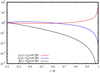 |
Fig. 1. Convective velocity profile uc, pressure scale height hp, and turbulent dynamical viscosity ηt calculated using an EZAMS model of HR 1099 and mixing length theory. |
For the surface magnetic flux density, we assume Bsurf = 1 kG. Details on the calculation of the Maxwell stress tensor and Reynolds stress tensor are described in Sect. 2. We adopt Av = AB = 0.1 as relative oscillation amplitudes for the velocity field and magnetic field inside the star.
3.1. Analytical approach
In order to understand the temporal evolution of the Applegate effect in the model presented here, we start with an analytical approach toward the most fundamental quantities involved in the mechanism. For a given set of functions that describe the oscillation of stellar parameters, the mechanism is controlled by the functions βnk and αnk, which can be calculated from the source term S(r, μ, t), which is in turn controlled by the function  as given by Eq. (29).
  consists of three terms:
-
a magnetic field term BiBϕ(r, t) that controls the mean magnetic field,
-
the Reynolds tensor Λiϕ(r, t) that describes the velocity field fluctuations, and
-
the Maxwell tensor Miϕ(r, t) that describes the magnetic field fluctuations.
 ), and
  . Furthermore, we employ a cyclic purely azimuthal magnetic field Bϕ(t) = Bsurf f(t) with constant amplitude Bsurf. We impose that all these quantities are tightly coupled and oscillate in phase. Under such conditions, all terms in
  have the same time dependence, implying
  for fixed r. Substituting into Eq. (15) yields βnk ∝ f(t)2. Given this result, we can evaluate Eq. (14): Following Lanza (2006) and employing that the first eigenvalues are typically associated with angular momentum redistribution modes on timescales shorter than the activity cycle of the star, we have αnk = βnk/λnk, which yields αnk ∝ f(t)2.
Finally, we arrive at
 (47)
(47)
The main insight of this exercise is the change in periodicity: In case of sinusoidal variations with period Pact in the magnetic field and the velocity field fluctuations, αnk, βnk, and Pdiss oscillate with half of the activity period to the leading order4 which is the observed binary modulation period Pmod as the quadrupole moment variation closely follows the dissipated energy (see following subsections). Another interesting result can be found by calculating the dimensionless quantity
 (48)
(48)
which compares the Reynolds tensor integral with the Maxwell tensor integral, quantifying the relative strength of the velocity field fluctuation amplitude versus the magnetic field fluctuation amplitude. Given Av = AB = 0.1, a surface magnetic field of Bsurf = 1 kG, and our EZAMS model of HR 1099, we have  , implying that the velocity fluctuations dominate the magnetic field fluctuations. The same holds for the zero-age main-sequence stars investigated in the parameter study in Sect. 3.6. As a result, the choice of Bsurf and AB does not significantly alter our results.
3.2. Eigenvalues and radial eigenfunctions
Figures 2 and 3 show the first four eigenfunctions ζ0k(r) and ζ2k(r) associated with the first four eigenvalues of λ0k and λ2k (see Table 2). A radial eigenfunction of order k has k nodes in [rb, R] (see, e.g., Lanza 2006).
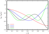 |
Fig. 2. Eigenfunctions ζ0k associated with the first four eigenvalues λ0k calculated for HR 1099 (see Sect. 3.2). These functions represent elemental angular momentum redistribution modes. |
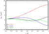 |
Fig. 3. Eigenfunctions ζ2k associated with the first four eigenvalues λ2k calculated for HR 1099 (see Sect. 3.2). These functions represent elemental angular momentum redistribution modes. |
Summary of the first ten eigenvalues of the radial equation for n = 0 and n = 2.
3.3. Eigenfunction normalization and k cutoff
For a fixed rb and assuming that all radial eigenfunction ζnk share one normalization parameter ζnk(rb), we find that the scaling relations ω ∝ ζnk(rb) and Pdiss ∝ ζnk(rb)2 hold. Consider ζnk(r) = ζnk(rb) ξnk(r) with dimensionless functions ξnk(r). Plugging into Eq. (9) and making use of the linearity of differentials yields
 (49)
(49)
which is equivalent to Eq. (9). This implies that for a fixed value of rb, n, and k, solutions for ζnk(r) with varying normalizations ζnk(rb) are multiples of one another. In particular, the eigenvalues λnk are constant. With this, we obtain for the dissipated energy
 (50)
(50)
and the kinetic energy dissipation rate becomes
 (51)
(51)
as the eigenvalues λnk are independent of the normalization chosen. In an analogous way, we can write
 (52)
(52)
for the angular velocity variation inside the star, which indeed implies ω(r, μ, t) ∝ ζnk(rb) because the functions αnk are invariant under variations of ζnk(rb).
As we investigate the question whether the Applegate effect – if operative – can explain the observed period variations in close binaries, we choose the following normalization strategy: First, we start with ζnk(rb) = 1 and calculate the eigenvalues λnk and the functions ζnk, βnk and αnk for n = 0 and n = 2 up to some maximum order kmax. The maximum order is determined by the eigenvalues, which have the dimension of inverse time and are associated with angular momentum redistributions on a timescale of 1/λnk (see Lanza 2005; Lanza 2006). For increasing orders of n and k, these timescales gradually shrink until they fall below the typical travel time of a soundwave when crosses the convection zone, which we calculate from
 (53)
(53)
where the speed of sound is
 (54)
(54)
assuming monoatomic gas. From this point, we therefore assume that higher orders are not able to contribute to the global angular momentum redistribution process. Depending on the details of the stellar interior, typicalk cutoffs range between 50 for evolved subgiants and >100 for red dwarfs. Given a k cutoff and the eigenfunctions ζnk (starting with ζnk(rb) = 1), βnk as well as αnk, we calculate the total energy dissipation Pdiss(t) and locate its maximum Pdiss, max. Given this, we adjust the eigenfunction normalization factor ζnk(rb) in order to have a maximum dissipated power equal to AP LHR1099. Using this normalization, the kinetic energy dissipation rate is limited to some fraction AP of the stellar power output LHR1099, which is typically on the order of 10%, and we can finally calculate the corresponding angular velocity variations inside the star.
3.4. Angular velocity variation and energy dissipation
The dissipated energy is calculated from Eq. (51) up to some radial order k. For k = 48, the timescale associated with the respective angular momentum redistribution mode is shorter than the calculated soundwave travel time. We fix the kinetic energy fluctuation limit to AP = 0.1 as described in the previous subsection. When αnk and ζnk are determined and our normalization to limit the kinetic energy dissipation is applied, we can calculate the effective angular velocity variation inside the star as functions of both time and stellar radius. In Fig. 4 we present the angular velocity changes inside the star for three different times between t = 0.05Pmod and t = 0.25Pmod. Starting from the state of rigid rotation at t = 0, the angular velocity variation builds up continuously with peak fluctuations of a few percent in the outermost layers of the star.
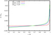 |
Fig. 4. Evolution of the equatorial angular velocity variation inside HR 1099 computed for three different times. |
3.5. Period modulation
In Fig. 5 we plot the calculated period variation in HR 1099 for Bsurf = 1 kG, a cycle length of Pact = 2 Pmod, a magnetic field fluctuation amplitude of AB = 0.1, and a velocity field fluctuation amplitude AV = 0.1 for three different cases of phase lag Δϕ between the radial and the azimuthal velocity and magnetic field fluctuations. The dissipated energy is limited to AP = 0.1 of the star’s luminosity. For Δϕ = 0, the oscillation is purely negative, that is, the quadrupole moment changes have a positive sign. On the other hand, for Δϕ = π/2, the period modulation oscillates between the positive and the negative regime, which is indicative of a cyclic transition between an oblate and a prolate state. Figure 6 shows the expected level of period variation in case of a surface magnetic field of 1 kG and varying fluctuation parameters AV, AB, and AP (see Sect. 2.2.1). Even with fluctuation amplitudes as high as AV = AB = AP = 0.5, which are not observed in HR 1099 (see Frasca & Lanza 2005), the resulting binary period variation amplitudes are still off by two orders of magnitude; no physically reasonable parameter range yields period variations as high as those observed in the system (9.0 × 10⁻⁵, Frasca & Lanza 2005). Given that the redistribution processes are almost entirely governed by convection (see Sect. 3.1), the only degree of freedom left to produce larger period variations is the convective velocity inside the star, for instance, through the mixing-length parameter αml. Reproduction of the observed modulation period of 35 yr imposes an activity cycle length of twice that value as the model predicts a 2:1 relation between the observed binary modulation period and the activity cycle length. Therefore, if the observed period variations are energetically and mechanically feasible, we would expect an activity cycle in HR 1099 of roughly 70 yr, while several authors claim to have found cycle lengths between 14.1 ± 0.3 yr and 19.5 ± 2 yr (see Lanza et al. 2006; Muneer et al. 2010; Perdelwitz et al. 2018, and references therein).
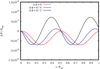 |
Fig. 5. Binary period variation amplitude calculated for a surface magnetic field of 1 kG, a cycle length of Pact = 2 Pmod, a magnetic field fluctuation amplitude of AB = 0.1, and a velocity field fluctuation amplitude AV = 0.1 for three different cases of phase shift Δϕ between the radial and azimuthal fluctuations. |
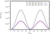 |
Fig. 6. Binary period variation in HR 1099 calculated for a surface magnetic field of 1 kG, a cycle length of Pact = 2 Pmod, no phase shift, and varying fluctuation parameters AV, AB, and AP. In a conservative scenario with AP = AV = AB = 0.1, the calculated binary period modulation amplitude is two orders of magnitude below the observed values (∼10−4). Increasing the velocity field fluctuation amplitude to AV = 0.3 at constant power dissipation AP = 0.1 only results in a slight increase of ΔP/P. Even for the rather extreme case of AP = AV = AB = 0.5, the produced period variations disagree with observations (see Frasca & Lanza 2005). |
3.6. Active component mass parameter study
We showed in the previous sections that RS CVns such as HR 1099 are not expected to produce significant levels of period modulation. We now expand our analysis to pre-cataclysmic PCEB systems (see, e.g., Zorotovic & Schreiber 2013), which have been proposed as potential Applegate systems by Völschow et al. (2016).
Consider a tidally locked binary system with a = 1 R⊙, consisting of a typical white dwarf primary with MWD = 0.5 M⊙ and a zero-age main-sequence secondary with varying mass. Just as in the previous sections, we assume a constant magnetic field of Bsurf = 1 kG and fix the fluctuation parameters to AP = AV = AB = 0.1 with a phase lag Δϕ = 0. For the modulation period, we assume Pmod = 15 yr. We varied the mass of the active component between 0.1 M⊙ and 0.6 M⊙ and calculated the amplitude of the orbital period variation using an EZAMS model of age t = 0. Figure 7 plots the expected period variation amplitude as a function of the active component mass. Between 0.1 M⊙ and 0.36 M⊙, we see a clear increasing trend toward higher binary period variation levels. For fluctuation parameters slightly above the fiducial 10% level, stars between 0.30 M⊙ and 0.36 M⊙ are expected to produce amplitudes ≃10−7, which is a typical order of magnitude observed in PCEB systems (Parsons et al. 2010; Zorotovic & Schreiber 2013; Völschow et al. 2016), while stars outside of this range only support low levels of period variations ≲10−7. For all simulated systems, the peak angular velocity variations are ≲1%.
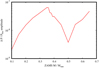 |
Fig. 7. Amplitude of binary period variation calculated for a surface magnetic field of 1 kG, cycle length of Pact = 2 Pmod, magnetic field fluctuation amplitude of AB = 0.1, velocity field fluctuations of AV = 0.1, and varying active component mass. The noticeable decrease in period modulation at 0.37 M⊙ coincides with the transition from fully convective to radiative-core stars. |
The physical explanation for the peak around M ≃ 0.35 M⊙ is the emergence of a radiative core, which shifts the boundary of the convective zone outward and reduces the total mass and angular momentum involved in the redistribution process. In Fig. 8 we plot the bottom of the convective zone as function of mass. Stars with M ≳ 0.37 M⊙ develop a radiative core, which reduces the domain available for angular momentum redistribution processes. While the calculated binary period modulation amplitudes again increase toward higher masses, the upper end of the investigated mass range may be affected by Roche-lobe overflow, which introduces additional effects that are not considered in our model. We also recall that fully convective stars with rb/R = 0 are strictly speaking not covered by the regular Sturm–Liouville problem, but the structure files adopted in our calculations for stars up to M = 0.36 M⊙ have relative convection zone depths of rb/R ≃ 0.01.
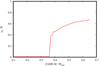 |
Fig. 8. Bottom of the convection zone rb as function of mass in our EZAMS stellar structure models. Stars up to 0.36 M⊙ are fully convective with non-zero convection velocities down to the innermost grid points. For higher masses, EZAMS predicts the emergence of a radiative core that takes up increasing fractions of the central region and reduces the total mass participating in the angular momentum redistribution processes. |
4. Conclusions and discussion
We presented a model that connects periodic fluctuations in the magnetic field and velocity field of the convection zone to periodic modulations of the quadrupole moment of the star, resulting in cyclic modulations of the binary period. Using the example of HR 1099, which has been discussed as one of the most promising Applegate candidates, we calculated the angular momentum redistribution modes ζnk(r) and considered the angular equation to calculate the αnk(t) and βnk(t) functions that are required to calculate the temporal evolution of the dissipated energy and the quadrupole moment, assuming that the star dedicates a fiducial fraction of AP = 0.1 of its luminosity to drive the Applegate mechanism. The order up to which we calculate the eigenfunctions is determined by a simple soundwave travel time argument. Our constant azimuthal field ansatz leads to a simple source function only controlled by the Λrϕ and Mrϕ components of the Reynolds and Maxwell tensors, where the former clearly dominates in the case of simple harmonic velocity and magnetic field fluctuations, which we control through the AB and AV parameters with fiducial values of 0.1.
In this model, harmonic oscillations of the magnetic field fluctuations and velocity field fluctuations on a timescale of the activity cycle Pact result in orbital period variations on a timescale of Pmod = 0.5 Pact. In other words, we expect that the activity cycle of any Applegate candidate satisfying our assumptions is double the observed binary modulation period, whereas alternative models predict a different ration (see, e.g., Applegate 1992; Lanza et al. 1998; Lanza & Rodonò 2004).
Furthermore, depending on the phase shift between the radial fluctuations and the azimuthal fluctuations, purely negative, positive or mixed quadrupole moment changes may be observed similar to findings by Rüdiger et al. (2002).
In line with previous work, we confirm that HR 1099 is not expected to produce period variations on the level observed today through the Applegate mechanism, which would require unphysically high field fluctuation amplitudes, angular velocity changes, and dissipated power. This is consistent with previous findings by Lanza (2005, 2006), who did not explicitly consider the temporal evolution of the mechanism.
While HR 1099 in particular and RS CVn systems in general seem highly unlikely Applegate candidates, our extensive parameter study identified short-period PCEBs with active component masses between 0.30 M⊙ and 0.36 M⊙ as the strongest Applegate candidates with expected period variation amplitudes similar to those typically observed in such systems, which are between 10−7 and a few 10−6 (see, e.g., Zorotovic & Schreiber 2013; Völschow et al. 2016). Consequently, we propose a careful reanalysis of PCEB systems with cyclic period variations to exclude the planetary hypothesis and find direct observational evidence that intrinsic effects such as quadrupole moment changes are at work.
To distinguish between Applegate modulations and period variations caused by planets through the light travel time effect (see, e.g., Pribulla et al. 2012), long-term measurements are required to determine the correlations between activity indicators, luminosity variations that are due to photospheric temperature changes, and the binary period modulation (Applegate 1992,). Changes in the rotational profile on the 1% level may lead to tiny deformations on a similar order of magnitude as the active component oscillates between an oblate and a prolate state, which is also expected to correlate with the activity cycle (Applegate 1992; Lanza et al. 1998; Rüdiger et al. 2002,). However, matters are complicated by spots and tidal deformations.
The model presented here is a significant step forward to understand the physics of the Applegate scenario. Nevertheless, it is still based on simplifying assumptions, such as a purely azimuthal magnetic field and the adoption of a mean-field framework. The Reynolds and Maxwell stress tensors do not self-consistently follow from a dynamo model either, but we adopt a (physically motivated) prescription for the kinetic and magnetic fluctuations that is externally imposed. Similarly, this approach still neglects effects such as viscosity quenching as a result of fast rotation, which may reduce the dissipated power and allow for higher levels of period variation in rapidly rotating systems (see Lanza 2006). Furthermore, our model does not guarantee the hydrodynamical stability of the differential rotation profile that emerges during the oscillation, although the maximum relative deviations from the state of rigid rotation are on the 2% level in HR 1099 and well below the 1% level in our PCEB parameter study (see Knobloch & Spruit 1982). Another limitation ist that we do not account for meridional circulation or for the effect of energy advection inside the star. Finally, additional quadrupole moment changes may occur as results of anisotropic Lorentz forces inside the star (Lanza et al. 1998).
While we cannot draw a final conclusion at this point, our framework nevertheless provides the most complete assessment of the Applegate mechanism so far, and it shows that a consideration of physical processes allows determining under which conditions the Applegate mechanism may be feasible. Our model yields testable predictions, suggesting that the Applegate mechanism may be favored for certain PCEB systems and disfavored in HR 1099. These predictions should be tested both on the observational side and through further refinement of the model to provide a clear picture where the Applegate mechanism is able to work.
The expression for the normalization constant can be derived by multiplying Eq. (5) with  , integrating as
  and making use of the orthogonality of ζnk for a fixed n with respect to the weight function ρr4, and the orthogonality of the Jacobian polynomials.
We chose HR 1099 for the sake of comparability with previous works by Lanza (2005); Lanza (2006) upon which our models is based.
Using the multiple-angle formula cos 4x = 1 − 8 sin2 x + 8 sin4 x, we see that f(t)2 and f(t)4 oscillate with the same amplitude and frequency, but are accompanied by a smaller oscillation with four times the frequency and 1/8 the amplitude.
Acknowledgments
We would like to express our gratitude to the anonymous referee for carefully reading our manuscript and providing us with valuable advice that improved the quality of our work. DRGS thanks for funding via Fondecyt regular (project code 1161247), the “Concurso Proyectos Internacionales de Investigación, Convocatoria 2015” (project code PII20150171) and the BASAL Centro de Astrofísica y Tecnologías Afines (CATA) PFB-06/2007.
References
- Applegate, J. H. 1992, ApJ, 385, 621 [NASA ADS] [CrossRef] [Google Scholar]
- Applegate, J. H., & Patterson, J. 1987, ApJ, 322, L99 [NASA ADS] [CrossRef] [Google Scholar]
- Beuermann, K., Dreizler, S., & Hessman, F. V. 2013, A&A, 555, A133 [NASA ADS] [CrossRef] [EDP Sciences] [Google Scholar]
- Brinkworth, C. S., Marsh, T. R., Dhillon, V. S., & Knigge, C. 2006, MNRAS, 365, 287 [NASA ADS] [CrossRef] [Google Scholar]
- Faulkner, J. 1971, ApJ, 170, L99 [NASA ADS] [CrossRef] [Google Scholar]
- Fehlberg, E. 1987, ZAMM – J. Appl. Math. Mech. / Z. Angew. Math. Mech., 67, 367 [CrossRef] [Google Scholar]
- Frasca, A., & Lanza, A. F. 2005, A&A, 429, 309 [NASA ADS] [CrossRef] [EDP Sciences] [Google Scholar]
- Gray, D. F., & Baliunas, S. L. 1994, ApJ, 427, 1042 [NASA ADS] [CrossRef] [Google Scholar]
- Hall, D. S. 1991, ApJ, 380, L85 [NASA ADS] [CrossRef] [Google Scholar]
- Han, Z.-T., Qian, S.-B., Irina, V., & Zhu, L.-Y. 2017, AJ, 153, 238 [NASA ADS] [CrossRef] [Google Scholar]
- Hardy, A., Schreiber, M. R., Parsons, S. G., et al. 2015, ApJ, 800, L24 [NASA ADS] [CrossRef] [Google Scholar]
- Horner, J., Wittenmyer, R. A., Hinse, T. C., et al. 2013, MNRAS, 435, 2033 [NASA ADS] [CrossRef] [Google Scholar]
- Knobloch, E., & Spruit, H. C. 1982, A&A, 113, 261 [NASA ADS] [Google Scholar]
- Kraft, R. P., Mathews, J., & Greenstein, J. L. 1962, ApJ, 136, 312 [NASA ADS] [CrossRef] [Google Scholar]
- Lanza, A. F. 2005, MNRAS, 364, 238 [NASA ADS] [CrossRef] [Google Scholar]
- Lanza, A. F. 2006, MNRAS, 369, 1773 [NASA ADS] [CrossRef] [Google Scholar]
- Lanza, A. F., & Rodonò, M. 1999, A&A, 349, 887 [Google Scholar]
- Lanza, A. F., & Rodonò, M. 2004, Astron. Nachr., 325, 393 [NASA ADS] [CrossRef] [Google Scholar]
- Lanza, A. F., Rodono, M., & Rosner, R. 1998, MNRAS, 296, 893 [NASA ADS] [CrossRef] [Google Scholar]
- Lanza, A. F., Piluso, N., Rodonò, M., Messina, S., & Cutispoto, G. 2006, A&A, 455, 595 [NASA ADS] [CrossRef] [EDP Sciences] [Google Scholar]
- Lebovitz, N. R. 1970, ApJ, 160, 701 [NASA ADS] [CrossRef] [Google Scholar]
- Matese, J. J., & Whitmire, D. P. 1983, A&A, 117, L7 [NASA ADS] [Google Scholar]
- Muneer, S., Jayakumar, K., Rosario, M. J., Raveendran, A. V., & Mekkaden, M. V. 2010, A&A, 521, A36 [NASA ADS] [CrossRef] [EDP Sciences] [Google Scholar]
- Nasiroglu, I., Goździewski, K., Słowikowska, A., et al. 2017, AJ, 153, 137 [NASA ADS] [CrossRef] [Google Scholar]
- Navarrete, F. H., Schleicher, D. R. G., Fuentealba, J. Z., & Völschow, M. 2018, A&A, 615, A81 [NASA ADS] [CrossRef] [EDP Sciences] [Google Scholar]
- Parsons, S. G., Marsh, T. R., Copperwheat, C. M., et al. 2010, MNRAS, 407, 2362 [NASA ADS] [CrossRef] [Google Scholar]
- Parsons, S. G., Gänsicke, B. T., Marsh, T. R., et al. 2013, MNRAS, 429, 256 [NASA ADS] [CrossRef] [Google Scholar]
- Perdelwitz, V., Navarrete, F. H., Zamponi, J., et al. 2018, A&A, 616, A161 [NASA ADS] [CrossRef] [EDP Sciences] [Google Scholar]
- Press, W. H., Teukolsky, S. A., Vetterling, W. T., & Flannery, B. P. 1992, Numerical recipes in FORTRAN. The art of scientific computing, 963, [Google Scholar]
- Pribulla, T., Vaňko, M., Ammler-von Eiff, M., et al. 2012, Astron. Nachr., 333, 754 [NASA ADS] [CrossRef] [Google Scholar]
- Qian, S.-B., Liu, L., Liao, W.-P., et al. 2011, MNRAS, 414, L16 [NASA ADS] [CrossRef] [Google Scholar]
- Rüdiger, G., Elstner, D., Lanza, A. F., & Granzer, T. 2002, A&A, 392, 605 [NASA ADS] [CrossRef] [EDP Sciences] [Google Scholar]
- Ulrich, R. K., & Hawkins, G. W. 1981, ApJ, 246, 985 [NASA ADS] [CrossRef] [Google Scholar]
- Verbunt, F., & Zwaan, C. 1981, A&A, 100, L7 [NASA ADS] [Google Scholar]
- Völschow, M., Schleicher, D. R. G., Perdelwitz, V., & Banerjee, R. 2016, A&A, 587, A34 [NASA ADS] [CrossRef] [EDP Sciences] [Google Scholar]
- Zorotovic, M., & Schreiber, M. R. 2013, A&A, 549, A95 [NASA ADS] [CrossRef] [EDP Sciences] [Google Scholar]
All Tables
Summary of the first ten eigenvalues of the radial equation for n = 0 and n = 2.
All Figures
|
Fig. 1. Convective velocity profile uc, pressure scale height hp, and turbulent dynamical viscosity ηt calculated using an EZAMS model of HR 1099 and mixing length theory. |
| In the text | |
|
Fig. 2. Eigenfunctions ζ0k associated with the first four eigenvalues λ0k calculated for HR 1099 (see Sect. 3.2). These functions represent elemental angular momentum redistribution modes. |
| In the text | |
|
Fig. 3. Eigenfunctions ζ2k associated with the first four eigenvalues λ2k calculated for HR 1099 (see Sect. 3.2). These functions represent elemental angular momentum redistribution modes. |
| In the text | |
|
Fig. 4. Evolution of the equatorial angular velocity variation inside HR 1099 computed for three different times. |
| In the text | |
|
Fig. 5. Binary period variation amplitude calculated for a surface magnetic field of 1 kG, a cycle length of Pact = 2 Pmod, a magnetic field fluctuation amplitude of AB = 0.1, and a velocity field fluctuation amplitude AV = 0.1 for three different cases of phase shift Δϕ between the radial and azimuthal fluctuations. |
| In the text | |
|
Fig. 6. Binary period variation in HR 1099 calculated for a surface magnetic field of 1 kG, a cycle length of Pact = 2 Pmod, no phase shift, and varying fluctuation parameters AV, AB, and AP. In a conservative scenario with AP = AV = AB = 0.1, the calculated binary period modulation amplitude is two orders of magnitude below the observed values (∼10−4). Increasing the velocity field fluctuation amplitude to AV = 0.3 at constant power dissipation AP = 0.1 only results in a slight increase of ΔP/P. Even for the rather extreme case of AP = AV = AB = 0.5, the produced period variations disagree with observations (see Frasca & Lanza 2005). |
| In the text | |
|
Fig. 7. Amplitude of binary period variation calculated for a surface magnetic field of 1 kG, cycle length of Pact = 2 Pmod, magnetic field fluctuation amplitude of AB = 0.1, velocity field fluctuations of AV = 0.1, and varying active component mass. The noticeable decrease in period modulation at 0.37 M⊙ coincides with the transition from fully convective to radiative-core stars. |
| In the text | |
|
Fig. 8. Bottom of the convection zone rb as function of mass in our EZAMS stellar structure models. Stars up to 0.36 M⊙ are fully convective with non-zero convection velocities down to the innermost grid points. For higher masses, EZAMS predicts the emergence of a radiative core that takes up increasing fractions of the central region and reduces the total mass participating in the angular momentum redistribution processes. |
| In the text | |
Current usage metrics show cumulative count of Article Views (full-text article views including HTML views, PDF and ePub downloads, according to the available data) and Abstracts Views on Vision4Press platform.
Data correspond to usage on the plateform after 2015. The current usage metrics is available 48-96 hours after online publication and is updated daily on week days.
Initial download of the metrics may take a while.