| Issue |
A&A
Volume 696, April 2025
|
|
|---|---|---|
| Article Number | A49 | |
| Number of page(s) | 12 | |
| Section | Astrophysical processes | |
| DOI | https://doi.org/10.1051/0004-6361/202453353 | |
| Published online | 02 April 2025 | |
Reconstruction of spider system’s observables from orbital-period modulations via the Applegate mechanism
1
Scuola Superiore Meridionale, Largo San Marcellino 10, 80138 Napoli, Italy
2
Istituto Nazionale di Fisica Nucleare (INFN), sez. di Napoli, Via Cinthia 9, I-80126 Napoli, Italy
3
INAF – Osservatorio Astronomico di Cagliari, Via della Scienza 5, I-09047 Selargius (CA), Italy
⋆ Corresponding authors; This email address is being protected from spambots. You need JavaScript enabled to view it.
, This email address is being protected from spambots. You need JavaScript enabled to view it.
, This email address is being protected from spambots. You need JavaScript enabled to view it.
Received:
9
December
2024
Accepted:
28
February
2025
Abstract
Redback and black-widow pulsars are two classes of peculiar binary systems characterised by very short orbital periods, very low-mass companions, and, in several cases, regular eclipses in their pulsed radio signal. Long-term timing revealed systematic but unpredictable variations in the orbital period, which can most likely be explained by the so-called Applegate mechanism. This relies on the magnetic dynamo activity generated inside the companion star and triggered by the pulsar wind, which induces a modification of the star’s oblateness (or quadrupole variation). This, in turn, couples with the orbit by gravity, causing a consequent change in the orbital period. The Applegate description is limited to providing estimates of physical quantities by highlighting their orders of magnitude. Therefore, we derived the time-evolution differential equations underlying the Applegate model; that is, we tracked such physical quantities in terms of time. Our strategy is to employ the orbital period modulations, measured by fitting the observational data, and implement a highly accurate approximation scheme to finally reconstruct the dynamics of the spider system in question and the relative observables. Among the latter is the magnetic field activity inside the companion star, which is still a matter of debate for its complex theoretical modelling and the ensuing expensive numerical simulations. As an application, we exploited our methodology to examine two spider sources: 47 Tuc W (redback) and 47 Tuc O (black widow). In this paper, the results obtained are analysed and then discussed in relation to the literature.
Key words: dynamo / gravitation / magnetic fields / binaries: eclipsing
© The Authors 2025
 Open Access article, published by EDP Sciences, under the terms of the Creative Commons Attribution License (https://creativecommons.org/licenses/by/4.0), which permits unrestricted use, distribution, and reproduction in any medium, provided the original work is properly cited.
This article is published in open access under the Subscribe to Open model. This email address is being protected from spambots. You need JavaScript enabled to view it. to support open access publication.
1. Introduction
Among the ∼3600 radio pulsars currently known1, about 14% are millisecond pulsars (MSPs). These are old neutron stars (NSs) endowed with relatively weak magnetic fields (B ≃ 107 − 109 G) and very short rotational periods (∼1 − 10 ms). MSPs represent the progeny of low-mass X-ray binaries (LMXBs), where the NS is spun up by the accreted matter (coming from the secondary star via Roche-lobe overflow) and finally attains extreme rotation rates. This is known and widely accepted in the literature as the recycling scenario (Bisnovatyi-Kogan & Komberg 1974; Alpar et al. 1982; Radhakrishnan & Srinivasan 1982; Bhattacharya & van den Heuvel 1991; Papitto et al. 2013).
Although MSPs are formed in binary systems, about 20% of them are isolated (Belczynski et al. 2010). The reason for this is still unclear and is a matter of debate (van den Heuvel & van Paradijs 1988; Rasio et al. 1989; Bhattacharya & van den Heuvel 1991). A possible explanation arose after the discovery of the first eclipsing binary pulsar, PSR B1957+20 (Fruchter et al. 1988), in which the companion star is constantly ablated by energetic particles and/or γ-rays produced by the pulsar wind (Kluzniak et al. 1988; van den Heuvel & van Paradijs 1988; Ruderman et al. 1989). This led astronomers to propose the so-called evaporation scenario, according to which the secondary star is ablated until it fully disappears, thus leaving an isolated MSP. However, successive estimates of the mass-loss rate showed that the evaporation timescale is likely much longer than the Hubble time, casting doubts on the effective occurrence of this phenomenon (Stappers et al. 1996a,b, 2001). Notwithstanding this, eclipsing binary pulsars became increasingly important for stellar and binary evolution studies. The recycling model, initially supported by the observation of accreting millisecond X-ray pulsars (AMXPs; see e.g. Wijnands & van der Klis 1998; Falanga et al. 2005), was ultimately confirmed by the discovery of three ‘transitional’ pulsars, (PSR J1023−0038, J1824−2452I, and J1227−4853); namely systems that have been observed swinging between radio-MSP and X-ray binary states (e.g. Papitto et al. 2013; Stappers et al. 2014).
Spider pulsars are a sub-class of binary MSPs characterised by tight (orbital period ≲1 d) and circular (eccentricities ≃10−3 − 10−4) orbits (see e.g., Romani et al. 2012; Pallanca et al. 2012; Kaplan et al. 2013) and a lightweight companion. Most (but not all) of them are also eclipsing binary pulsars. Depending on the mass mc of the companion, they can be further divided into two distinct classes (Roberts 2013): black widows have degenerate companions with mc ≲ 0.1 M⊙, whereas redbacks have semi-degenerate companions with mc ≃ 0.1 − 0.4 M⊙. The evolutionary scenario of these two types of binary systems has long been discussed, and it is now widely accepted to occur through irradiation processes (Podsiadlowski 1991; D’Antona & Ergma 1993; Bogovalov et al. 2008, 2012; Chen et al. 2013; Smedley et al. 2015, and references therein).
The long-term timing of several spiders has revealed that they often show significant modulations of their orbital periods, and sometimes also of their projected semi-major axes (see e.g. Shaifullah et al. 2016; Ng et al. 2018). These variations generally manifest themselves as recurrent, but not strictly periodic, cycles. These observational clues lead to the exclusion of apsidal motions as dynamical explanations (Sterne 1939) and the presence of third bodies (van Buren 1986). Instead, a plausible reason can be the magnetic activity inside the companion star (Hall 1990), closely linked to the dynamo action due to the presence of differential rotation and convective zones.
Spider systems are usually found in quasi-tidally locked configurations, occurring when there is no relevant angular momentum transfer between the companion star and its orbit around the pulsar. This is due to the tidal force acting between the co-orbiting bodies through the pulsar irradiation-driven winds (see e.g. Applegate & Shaham 1994; Bogdanov et al. 2005), entailing the tidal dissipation of the pulsar on the companion (known as a tidally powered star; see e.g. Balbus & Brecher 1976; Kochanek 1992; Zahn 2008) and synchronous rotation (one hemisphere of a revolving body constantly faces its partner).
A possible explanation for the orbital period variations relies on the Applegate mechanism (Applegate & Patterson 1987; Applegate 1992b,a), where magnetic cycles induce deformations on the companion star shape, thus altering its quadrupole moment, consequentially causing gravitational acceleration and orbital period modulations. This phenomenon is triggered by the irradiation-driven winds from the pulsar, which generates a spin torque on the companion. This in turn induces tidal dissipation and energy flow, which powers the magnetic dynamo (Applegate & Shaham 1994).
The observed orbital period and projected semi-major axis modulations can be influenced by other effects that are intrinsic to the system or caused by kinematic reactions relative to the observer motion (e.g. emission of gravitational waves, Doppler corrections, mass loss of the binary, and tidal bulge forces), which Lazaridis et al. (2011) estimated to be orders of magnitude smaller than those caused by the gravitational quadrupole-moment activity. On the other hand, Lanza et al. (1998), Lanza & Rodonò (1999) proposed an alternative explanation to the gravitational quadrupole-moment variations. Their model applies the tensor virial theorem (Chandrasekhar 1961) to a general magnetic field geometry to formalise, through an integral approach, the variations in oblateness. This implies a distributed non-linear dynamo in the convective envelopes of the companion star, which affects not only the quadrupole moment, but also the differential rotation.
The Applegate mechanism is still the most quoted explanation for its good agreement with the observations, whose measured amplitudes of period modulations are ΔP/P ∼ 10−5 (over timescales of decades or longer), whose companion star’s variable luminosity is over the ΔL/L ∼ 0.1 level, and whose differential rotations are of the order of ΔΩ/Ω ∼ 0.01. These values are common in spider systems (see e.g. Ridolfi et al. 2016; Freire et al. 2017).
More recently, Voisin et al. (2020a,b) improved the Applegate picture, also taking into account relativistic corrections. They proposed a detailed model for describing the motion of spider binary systems that allows us to accurately estimate the observed ΔP variations with the final objective of improving the timing solution of these gravitational sources.
Having solid theoretical assessments to describe spider systems represents a powerful means to (i) better understand the stellar magnetic activity, (ii) obtain insights into the dynamo processes, and (iii) acquire more information on the companion stars’ equations of state. In particular, the structure and generation of the magnetic field in low-mass stars are still not clear and need to be investigated. The surface magnetic field is thought to be of the order of several kilogauss and can be directly observed (see Fig. 1 in Han et al. 2023). Instead, the interior fields are based on contrasting theoretical analyses strongly depending on the considered model (see e.g. Yadav et al. 2015; Feiden & Chaboyer 2014; MacDonald & Mullan 2017).
In this work, we employed the Applegate mechanism, which, besides describing the phenomenology behind the spider pulsar, also provides an estimate of the order of magnitude of some related physical variables (e.g. luminosity, differential rotations, quadrupole moment, etc.). We propose a dynamical formulation of the Applegate model, where the gravitational source and physical quantities’ dynamics are tracked point by point during their time evolution. In addition, we exploited an inverse approach counter-current with respect to the strategies followed in the latest papers (see e.g. Voisin et al. 2020a,b). Indeed, rather than finding a physical justification for the ΔP variations, we took its profile from the long-term observations to reconstruct the gravitational source and related observables’ dynamics. The approach we adopted in this work follows the BTX phenomenological model (extension of Blandford & Teukolsky (BT) model, Blandford & Teukolsky 1976; Bochenek et al. 2015), which allows one to fit the observational data within a precise timing baseline. This scheme gives rise to a set of coupled ordinary differential equations with respect to time, involving the orbital separation and quadrupole moment. However, the ensuing dynamical system is still difficult to solve analytically. Therefore, we also developed a mathematical procedure that provides highly accurate approximate analytical solutions. This methodology allows for an easy accomplishment of the proposed goals.
The paper is structured as follows. In Sect. 2, we describe the features of our dynamical model and derive the equations of motion; in Sect. 3, we propose a reasonable approximation pattern to infer an analytical solution; in Sect. 4, our achievements are applied to black-widow and redback systems; finally, in Sect. 5, we conclude with some discussions and future perspectives.
2. The model
We present the dynamical version of the Applegate mechanism, which reports the order of magnitude of the physical observables underlying the dynamics of black-widow and redback binary systems. This model is further enhanced by incorporating the orbital period modulations’ profiles, which are derived from observations. This gives rise to a set of coupled and non-trivial ordinary differential equations. We also introduce the explicit formulae of some physical variables, of which plotting the profiles was the goal of our work.
We dealt with binary sources composed of a pulsar of mass mp and a companion star of mass mc and radius Rc. The two bodies were both treated as test particles, even if the companion star should be considered as extended to account for changes in shape. However, to simplify the mathematical treatment, we still regard this object as a test body, and we trust the quadrupole variable to characterise the variations of matter distribution within the star. In Fig. 1, we show a cartoon featuring the geometry of the problem under investigation.
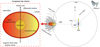 |
Fig. 1. Illustration of typical spider binary system. An MSP and a companion star are in a tidally locked configuration, moving in synchronous rotations on quasi-circular and tight orbits. They are separated by a distance of rs(t) in a plane orthogonal to the orbital angular-momentum vector L, which is conserved during the binary system’s motion. The irradiation-driven wind from the MSP heats through a tidal dissipation the companion star, which starts to evaporate, thus losing mass. This is the eclipsing material, which acts as an obstacle to the radio signal detected by a telescope located far from the binary system. In the dashed red box we sketch the companion star’s interior. This zone is characterised by a convective envelope, where the fluid in it is highly conductive. Furthermore, the pulsar wind triggers the differential rotation of the companion star, which induces a magnetic activity through a dynamo action. The subsurface magnetic field is responsible for breaking the hydrostatic equilibrium inside the star, inducing quadrupole moment changes. We note that the external magnetic field is expected to be locally poloidal, while the sub-surface field is toroidal. |
The definitions of some of the above parameters require additional clarifications. The companion star’s mass, mc, is not strictly constant over time, as it gradually decreases due to the mass loss driven by the pulsar wind. However, the fraction of matter lost over the observational period is so small (around 10−10 M⊙/yr)2 that it is reasonable to approximate mc through a constant value. Similarly, the radius of the companion star, Rc, is not fixed; it varies as the shape of the star changes due to quadrupole variations. Therefore, the definition of Rc refers to the companion star’s radius at rest. These fluctuations in the size dimension can be quantified, and their relative magnitude is estimated to be about 5 − 7% with respect to Rc (Applegate 1992a)3.
This section opens by briefly recalling the Applegate mechanism in Sect. 2.1, representing the core of our work. In the construction of the model, we made use of the two reference frames (RFs) described in Sect. 2.2, which allowed us to conveniently deal with the ensuing dynamics. The equations of motion are presented in Sect. 2.3. We conclude by deriving the formulae of some fundamental physical observables involved in this scenario in Sect. 2.4.
2.1. Applegate mechanism and dynamo action
Applegate (1992a) proposed a mechanism to explain the orbital-period modulations in eclipsing binary systems as a consequence of the magnetic activity inside the secondary star, triggered by the pulsar wind. For spider binary systems (i.e. black widows and redbacks), the lighter body plays the role of the active star. The main idea underlying this approach is based on the magnetic activity cycle, which represents the engine that causes a redistribution of the angular momentum inside the star, thus modifying its oblateness (see e.g. Warner 1988; Lanza & Rodonò 2002; Donati et al. 2003; Lanza 2006; Bours et al. 2016). This induces a variation in the radial component of the gravitational acceleration via the gravitational quadrupole-orbit coupling, thus entailing the orbital period modulations, which we eventually detected.
This magnetic activity seems to be powered by a dynamo action, that is a process of magnetic-field generation through the inductive response of a highly-conductive fluid. Indeed, there is a conversion of mechanical energy into a magnetic one by stretching and twisting the magnetic-field lines (Parker 1955). All of the aforementioned effects are driven by the sub-surface magnetic field, which is located within the star’s convective zones.
The dynamo action is the alternation of two phenomena inside the star: (1) the sheared differential rotation at different latitudes contributes to the transformation of an initially poloidal magnetic field into an enhanced toroidal one through the Alfvén theorem (also known as the Ω effect; see e.g. Parker 1955, 1979; Browning et al. 2006); and (2) the combined action of cyclonic convection, buoyancy, and Coriolis forces turns the toroidal magnetic field back to the poloidal one, thus completing the cycle (also known as the α effect; see e.g. Parker 1955, 1979; Choudhuri et al. 1995; Charbonneau & Dikpati 2000; Browning et al. 2006).
The dynamo model is usually gauged on the solar magnetic activity, as it shares profound similarities with the problem under investigation. We know from observations of the Sun that the period of the sunspot cycles (connected to the solar sub-surface magnetic activity) is about 11 years (Baliunas & Vaughan 1985), but this value can be of a much longer duration in spider systems. From this consideration and since various cycles can have different durations, we can conclude that the magnetic activity leads to systematic, but not strictly periodic, changes in the active star, subsequently causing the observed orbital period variations.
2.2. Reference frames
Spider systems are fairly tight, implying highly circular orbits. Furthermore, the tidal friction predominately leads to a synchronisation of the spin and orbit of the binary system; i.e., rotational and orbital angular momentum vectors are aligned and also have the same module. The dynamics occurs in the plane 𝒫 orthogonal to the direction of the orbital angular momentum. We neglected any additional perturbing effects that could potentially lead to three-dimensional motions outside the 𝒫 plane.
The dynamics can be described in two RFs, with both having their origins in the binary system’s centre of mass (CM; see Fig. 2). These are described below.
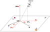 |
Fig. 2. We display two RFs: ℛCO (black) and ℛS (red). |
-
Orthonormal corotating RF, ℛCO = {x,y,z}: the z-axis is orthogonal to 𝒫, where the x- and y-axes are placed. The x-axis is always directed along the line connecting the two bodies and pointing towards the companion star. This RF co-rotates with the binary system, so the motion in it is always static. The only variations occur along the x-axis, reducing thus the whole dynamics to just one dimension;
-
Orthonormal static RF, ℛS = {xS,yS,zS}: zS ≡ z, where the xS-axis is directed towards the position of a static and non-rotating observer at infinity O∞, namely from CM to O′∞ (being the projection of O∞ on 𝒫). This RF is fixed in space, and all quantities measured in it are labelled by a subscript S.
These RFs are related by the map T : ℛCO → ℛS. It is determined by employing polar coordinates, the radius rS(t) (coincident with the coordinate x), and the polar angle θS(t), where t is the time. More explicitly, this transformation reads as
 (1)
(1)
2.3. Equations of motion
Our model is governed by the gravitational quadrupole-orbit dynamics (see Sect. 2.3.1) and the time-variation of the quadrupole moment (see Sect. 2.3.2). This differential problem can be solved if it is accompanied by the appropriate initial conditions (see Sect. 2.3.3). We stress again that, even though our model is fully based on the Applegate mechanism, the related dynamical equations of motion have never been written in the literature.
2.3.1. Gravitational quadrupole-orbit coupling dynamics
The two bodies are influenced by their mutual gravitational attraction and the companion star’s gravitational quadrupole-orbit coupling. The problem is first framed in ℛCO, where the pulsar has the coordinates ( − xp, 0, 0), while those of the companion star are (xc, 0, 0).
The force acting on the pulsar is Fp, which is the sum of the gravitational force and the quadrupole-moment contribution Q(t)4 from the companion star, namely (Applegate 1992a)
 (2)
(2)
Instead, the force acting on the companion star is Fc, simply given by the gravitational force from the pulsar:
 (3)
(3)
We define the relative coordinate system x = xc − xp and the relative acceleration  (the overdot stands for the derivative with respect to the time t), together with the total MTOT = mp + mc and reduced μ = mpmc/MTOT masses. After appropriately manipulating Eqs. (2) and (3), we obtain
 (4)
(4)
Changing RF through the transformation T, we rewrite the above dynamics in polar coordinates in ℛS. Considering the angular component, we obtain the following equation of motion:
![Mathematical equation: $$ \begin{aligned} \frac{1}{r_{\rm S}(t)}\frac{\mathrm{d}}{\mathrm{d} t}\left[\mu \ r_{\rm S}(t)^2\ \dot{\theta }_{\rm S}(t)\right] = 0, \end{aligned} $$](/articles/aa/full_html/2025/04/aa53353-24/aa53353-24-eq6.gif) (5)
(5)
which immediately entails  . Here, L is the module of the conserved angular momentum L of the system along the zS-axis, which can be calculated using the initial conditions.
The problem is defined in the time frame [t0, t1]. However, since the setting is invariant under time shifts, we can consider, without loss of generality, the following normalised interval: [0,1]5. The map connecting [t0, t1] with [0,1] is given by
![Mathematical equation: $$ \begin{aligned} t\in [t_0,t_1]\rightarrow \frac{t-t_0}{t_1-t_0}\in [0,1]. \end{aligned} $$](/articles/aa/full_html/2025/04/aa53353-24/aa53353-24-eq8.gif) (6)
(6)
We stress that T0 is the reference time, usually coincident with the transition to the orbit periastron6. This is the moment where we extracted the parameters that would correspond to the initial time T0* = (T0 − t0)/(t1 − t0). However, the observations begin at t0 < T0. Therefore, it is reasonable to set the initial conditions at T0 and extend our solutions back to the earlier time, t0.
The angle θS(t) can be calculated through the formula θS(t) = ω(t)(t − T0*), where ω(t) is the angular frequency. Since the system is very tight, the bodies move on quasi-circular orbits with relative angular velocity (see Eq. (5) in Applegate 1992a):
 (7)
(7)
Therefore, the angular frequency ω(t) can be estimated by applying the formula for (quasi-)circular motion (Applegate 1992a):
 (8)
(8)
It is important to note that  , since
 (9)
(9)
However, at the beginning (i.e. for t = T0*) we have  .
.
Instead, for the radial component, we obtain
 (10)
(10)
where the change of RF can be seen by the appearance of the centrifugal force (first term on the right hand side). This dynamical system is composed bof a second-order ordinary differential equation (10); this should be complemented by the dynamics of Q(t),7 which is disclosed in the next section.
2.3.2. Quadrupole dynamics
The Applegate mechanism foresees that there are two kinds of deformations due to the magnetic activity, which can be classified into (1) distortions, which modify the hydrostatic equilibrium in the deformed configuration; and (2) transitions, which cause changes from one fluid hydrostatic configuration to another. Applegate (1992a) explained that distortions are not astrophysically relevant, because the weak magnetic fields (∼105 − 106 G) cannot supply enough energy for the star deformations to reproduce the orbital-period modulation timescales (see text following Eq. (23) for a more detailed discussion). Therefore, we considered modifications due to the transitions, where the dynamics of a rotating star strongly depends on the matter distribution within it and its angular momentum J, which influences the quadrupole-moment variations in agreement with the observed timescales.
A fundamental role is played by its external layers, which contribute to spinning up the star, making it more oblate (i.e. enhancing its quadrupole moment; Applegate 1992a). Therefore, the magnetic activity makes it possible for a torque to arise and develop, which acts on the spin of the companion star to extract angular momentum (Applegate 1992a; Applegate & Shaham 1994). From Eq. (26) in Applegate (1992a), the companion star’s quadrupole moment changes according to the following formula:
 (11)
(11)
where Ω is the angular velocity of the outer layers, which can be reasonably calculated through the Keplerian angular velocity:
 (12)
(12)
The variation of J is caused by the spin torque, because the irradiation-driven wind from the pulsar generates a ram pressure contributing to the spin-up of the companion star. Employing Eq. (27) in Applegate (1992a), the time-variation of J is8
 (13)
(13)
where ΔP(t) is also known as orbital-period modulations. Therefore, the resulting differential equation ruling the dynamics of Q(t) is obtained by substituting Eq. (13) into Eq. (11), namely
 (14)
(14)
2.3.3. Initial conditions
Our model is governed by a system of the ordinary differential Equations (10) and (14). It must be complemented by the initial conditions at the time t = T0* to find a unique solution; these conditions are
 (15)
(15)
where a is the initial separation between pulsar and companion star and Q0 = 0.1mcRc2/3 is the initial quadrupole (cf. Eq. (25) in Applegate 1992a). The radial velocity is determined employing Kepler’s third law in its differential form, as the two bodies’ orbits are Keplerian at every moment in time. The conditions (15) imply (cf. Eqs. (7) and (8))
 (16)
(16)
2.4. Physical observables
This section provides some physical observables related to spider systems. To achieve this objective, we must first solve Eqs. (10)–(14), as we need rS(t) and Q(t), which are already fundamental physical quantities. We focused on the following quantities in our work: orbits pertaining to the two bodies (see Sect. 2.4.1), orbital period (see Sect. 2.4.2), magnetic-field intensity (see Sect. 2.4.3), and luminosity variability (see Sect. 2.4.4).
2.4.1. Two-body orbits
An important feature of a binary system is to understand the evolution of the orbit. Since the two bodies are tidally locked and synchronised, we need to determine the separation rS(t) and the quadrupole moment Q(t) to calculate ω(t) (cf. Eq. (8)), which in turn provides the evolution of the polar angle θS(t). Therefore, passing in cartesian coordinates, the orbit is obtained by plotting
![Mathematical equation: $$ \begin{aligned} (r_{\rm S}(t)\cos \theta _{\rm S}(t),r_{\rm S}(t)\sin \theta _{\rm S}(t)),\qquad t\in [0,1] ,\end{aligned} $$](/articles/aa/full_html/2025/04/aa53353-24/aa53353-24-eq21.gif) (17)
(17)
where t is given by Eq. (6).
2.4.2. Orbital period
The orbital period P(t) can be estimated in two ways: (1) once we solve the system, we determine the orbit and we then calculate it; (2) it can be obtained a priori by fitting the observational data. In this work, we used the latter approach, as we aim to reconstruct the dynamics of the physical observables.
In the a priori approach we first calculated ΔP(t) = P(t)−P0, where P0 is estimated via Kepler’s third law, namely
 (18)
(18)
The formula used to fit ΔP(t) (generally expressed in seconds) is
 (19)
(19)
where f0 = 1/P0 and
 (20)
(20)
The fitting procedure was performed in the interval [t0, t1], expressed in MJD. Furthermore, the coefficients {fi}i = 0n represent the higher order frequency derivatives, and n is the order of terms involved in the fit. The parameters {fi}i = 0n and T0 are obtained as a timing solution of a BTX model provided by the TEMPO or TEMPO2 software. The value of n changes from a pulsar to another, since it is the number of the reliably measured time derivatives of the orbital period and depends on various aspects; these include the time interval covered by the radio observations, the typical uncertainty on the measured pulses’ times of arrival; the r.m.s of the timing residuals; and more (see e.g. Ridolfi et al. 2016; Freire et al. 2017). We also note that  , which is useful for computing
  in Eq. (15). For what follows, it is useful to define the constant quantity
![Mathematical equation: $$ \begin{aligned} \mathcal{A} =\langle \frac{\Delta P(t)}{P(t)} \rangle _{[t_0,t_1]}, \end{aligned} $$](/articles/aa/full_html/2025/04/aa53353-24/aa53353-24-eq27.gif) (21)
(21)
where ⟨ ⋅ ⟩[t0, t1] is the time average in the interval [t0, t1].
2.4.3. Magnetic-field intensity
In the Applegate mechanism, the magnetic energy is the main source of support to provide the necessary torque for the exchange of angular momentum between the shells of the companion star (and consequently changes in the quadrupole moment). In this scenario, the magnetic field does not decay in rapid times, because observations so far have not detected orbital-period variations over short timescales. This phenomenon represents an indirect probe for the internal magnetic-field dynamics within active stars. Therefore, spider pulsars are natural laboratories and ideal systems for investigating the magnetic dynamics in low-mass stars, since this topic is still matter of discussion.
The variation of the sub-surface (toroidal) magnetic-field intensity with respect to that of the unperturbed (i.e. Q(t) = 0) configuration can be estimated through the following formula (see for further details Eq. (33) in Applegate 1992a):
 (22)
(22)
where Pma is the magnetic period, which is specific for each spider system. It is computed by searching for the maxima (or minima) in the ΔP(t) profile, whose average distances allows us to extract a mean value. We stress that Eq. (22), as derived by Applegate (1992a), only provides an estimate of the magnetic-field intensity. In the original formula, ΔP is interpreted as a (constant) positive quantity. Since in our case ΔP(t) assumes both positive and negative values, as well as zero, it is more appropriate to insert the absolute value to derive a realistic result. In addition, inspired by the ΔP(t) profile, it is more opportune to calculate (through Eq. (22)) the variations ΔB(t), rather than B(t). We stress ΔB(t) = B(t)−B0, where B(t) is due to the quadrupole variations, whereas B0 stays for the unperturbed case. In order to guarantee regular behaviours and attain negative values, we added the function sign of the ΔP(t) outside the square root. We made the function continuous, but it is not differentiable in the points crossing the zero line. This is the best we can achieve, as we are ignorant to the magnetic activity occurring inside the companion star.
We considered a rough estimate of the magnetic field B0 proposed by Applegate, which was obtained by substituting, in Eq. (22), rS(t) with its initial value a and ΔP(t) with the trend 𝒜P0 (cf. Eq. (21)). Therefore, by performing these calculations, we obtain
 (23)
(23)
2.4.4. Luminosity variability
Another non-uniform periodic mechanism is related to the physics of the luminous variability inside the active star. This cycle is divided into the two phases (Applegate & Patterson 1987; Applegate 1992a; Applegate & Shaham 1994) described below.
-
(i)
The angular-momentum transfer leads to an enhancement of the kinetic energy, because it is spent to power the differential rotation between the inner part and the outer layer of the active star. This activity leads the star to spin-up at the expenses to lower the luminosity.
-
(ii)
When the angular-momentum transfer decreases, the active star rotates as a solid body. This causes the star to spin down, with a consequent increment in its luminous intensity.
The alternation of the two cycles gives rise to the observed luminous modulations. In addition, in the entire process there is also a weak dissipation, because the orbital period tends to weakly decrease with time. However, this dissipative effect was not taken into account in this model due to its negligible contributions.
The energy emitted by the companion star can be estimated through (see Eq. (28) in Applegate 1992a, for details)
 (24)
(24)
where Ωdr = Ω(1 − η) with an efficiency of η = 0.66 (see Fig. 1 in Yoshida 2019), and Is represents the moment of inertia of the outer layer considered as a shell; this is given by (Applegate 1992a)
 (25)
(25)
where Ms ≈ 0.1mc is the outer-layer mass (Applegate 1992a). Therefore, the luminosity modulation can be easily calculated as
 (26)
(26)
where Δℒ(t) represents the difference between the luminosity due to the quadrupole variations and the constant luminosity of the star without altering its shape. This formula allowed us to track the companion star’s luminosity with respect to the unperturbed configuration during the time evolution and to monitor how it changes in terms of the orbital period modulations.
Finally, we provide an estimate of the unperturbed luminosity, expressed by the following formula (using Eq. (26), where we substituted rS(t) with a and ΔP(t) with 𝒜P0):
 (27)
(27)
3. Methodology
The spider system dynamics is described by two coupled non-linear differential equations ((10)–(14)), where the analytical solution is too difficult to determine, and therefore numerical routines must be exploited. We note that if we follow the a posteriori approach (see Sect. 2.4.2), we must have a precise temporal trend for dΔP/dt, which is related to the sub-surface magnetic field of the active star. This is a very demanding task for several reasons (see Dobler et al. 2006; Browning 2008, and references therein): (1) there are theoretical uncertainties about the microphysics inside low-mass stars; (2) there is a high computational cost to performing magnetohydrodynamic (MHD) simulations; (3) several models exist, based on different simplifications and hypotheses.
In order to avoid the aforementioned issues, we used the a priori approach (see Sect. 2.4.2) founded on obtaining the function ΔP(t) by fitting the observational data. However, even after substituting the orbital period modulations (19) in the equations of motion, the ensuing dynamics is still too cumbersome to be analytically integrated. Therefore, if we want to avoid numerical integrations, some approximation schemes must be employed.
We present a methodology to derive an approximate analytical solution of Eqs. (10) and (14) in Sect. 3.1. We comment on the approximation accuracy with respect to the original (unaffected) equations in Sect. 3.2. We conclude by specifying the inputs and outputs of our model in Sect. 3.3.
3.1. Approximation strategy
To better analyse the problem, one should bare in mind that the motion is quasi-circular. Therefore, we can assume the validity of Kepler’s third law in each point. Differentiating it, we obtain, at the first order in ΔP and ΔrS,
 (28)
(28)
Substituting the relations
 (29)
(29)
into Eq. (28) and neglecting second-order terms, we have
 (30)
(30)
which completely determines the function rS(t) in terms of the orbital-period modulations ΔP(t), taken from the observations.
Equation (14) is the only differential relation left, which must be solved numerically. However, we can avoid this last integration by sampling rS(t) and ΔP(t) functions at several points. Then, we fit them with highly accurate polynomials with n + 1 coefficients, using the same n of the TEMPO coefficients {fi}i = 0n, because this allows a drastic reduction of the approximation errors. The fitting procedure occurs in the interval [0,1], since this gives more accurate results. Using the transformation (6), we can then map the ensuing polynomial in the interval [t0, t1].
In this case, Eq. (11) can be analytically written as
 (31)
(31)
where the coefficients ai are real numbers that can be explicitly calculated when we have the polynomials of rS(t) and ΔP(t). The integer m depends on the final polynomial order obtained by multiplying the two aforementioned polynomials.
3.2. Approximation accuracy
To check the reliability of the result we found, we needed to compare our approximation with the numerical solution of Eqs. (10) and (14). For this purpose, we used Mathematica 13.1 and Python 3 to confidently validate our calculations.
In Mathematica 13.1, we employed the function NDSolve and exploited the methods StiffnessSwitching and ExplicitRungeKutta, selecting a precision and accuracy level of ten and a maximum step size of 10−6 in the interval [0,1]. Then, we plotted rS with several points (∼800), while Q(t) can be displayed by employing significantly fewer points (∼100).
In Python 3, we used the integration routine dop853, which is the Dormand-Prince algorithm implemented within the class of explicit Runge-Kutta methods of eight orders Dormand & Prince (1980), Press et al. (2002). We selected absolute 10−20 and relative 10−10 tolerances within [0,1] with a step-size of 10−7. The two approaches are in agreement, since they give the same results.
The approximate radius differs from the numerical one, because the latter contains mild oscillations (since the orbit is quasi-circular) and an overall modulation on the time span [0,1]; whereas the former features only the modulation on [0,1] (since the orbit is considered circular). Instead, the quadrupole moment between the two approaches coincides with mean relative errors (MREs) < 10−5%. Therefore, our solution is consistent.
3.3. Inputs and outputs of the model
Our approach relies on the analytical (highly accurate approximation) formulae of rS(t) and Q(t). This allowed us to quickly compute the evolution of the associated physical observables reported in Sect. 2.4. Our methodology is also flexible, because it can be used in an opposite manner. Indeed, knowing the trend of some physical variables (e.g. the luminosity), we could extract the orbital period modulations and then determine all the other quantities.
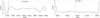 |
Fig. 3. Orbital-period modulations of 47 Tuc W and 47 Tuc O, obtained from the fitting of the observational data (see Table A.1). The vertical dashed line marks the position of T0. |
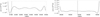 |
Fig. 4. Discrepancy of actual separation among the bodies with respect to the initial datum. The vertical dashed line marks T0. The order of the sources is placed as in Fig. 3. |
The input values of our model are
 (32)
(32)
where mp can be set as equal to the value of a standard NS (i.e. mp = 1.4 M⊙), and if we know the spider class, we can assign average values of mc and Rc. The initial orbital separation a can be calculated via Kepler’s third law (cf. Eq. (18)) if we know that P0 = 1/f0, mp, mc. Depending on the goal, we generally have n + 6 input parameters, which can eventually be lowered to n + 3. The output parameters of our model are
 (33)
(33)
4. Results
As an application of our model, we considered the spider systems 47 Tuc W (redback) and 47 Tuc O (black widow). The input parameters and the TEMPO coefficients of these two physical systems are reported in Table A.1. In Fig. 3, we display the orbital-period modulations of these two sources (see for more details Ridolfi et al. 2016; Freire et al. 2017). The polynomial approximations described in Sec. 3.1 are reported in Appendix A. In this section, we first compare the results from the two sources in Sect. 4.1, and then in Sect. 4.2 we analyse how we determined the associated parameters after detecting a spider source.
4.1. Comparison between 47 Tuc W and 47 Tuc O
We analysed 47 Tuc W and 47 Tuc O’s dynamics via our model through the related physical variables’ profiles (33). We also highlight common features (see Sect. 4.1.1) and diversities (see Sect. 4.1.2).
4.1.1. Analogies
The radius follows the same trend of the orbital period modulations (cf. Eq. (29) and (30)), but with very mild oscillations (see Fig. 4). This feature also transmits to the orbits, which, besides to be quasi-circular, admit a very narrow advancement with respect to the long time baseline. Instead, the quadrupole moment behaves in the opposite way (see Fig. 5), because the orbit shrinks (enlarges) as the quadrupole increases (decreases).
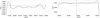 |
Fig. 5. Evolution of quadrupole moment Q(t)/Q0, where the horizontal dashed line is set at 1 and the vertical dashed line marks T0. The order of the sources is as in Fig. 3. |
The magnetic-field variability, compared to other observables, features a very oscillating trend scanned by the magnetic-activity period Pma (see Fig. 6). The variable magnetic field B(t) crosses the zero line at the points where ΔP(t) nullifies, corresponding to moments when the magnetic field matches the initial star’s intensity. Since the provided formula is a rough estimate of the sub-surface magnetic-field strength (with an offset value B0), we anticipate that MHD simulations could offer a similar but more detailed and accurate representation.
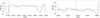 |
Fig. 6. Variation of magnetic-field intensity ΔB(t). The horizontal dashed line is B0 (cf. Eq. (23)), whereas the vertical dashed line marks T0. The order of the sources is as in Fig. 3. |
Finally, the luminosity is ruled by the quadrupole moment (cf. Eq. (26)), where the zero points coincide with the luminosity of the initially observed star (see Fig. 7). For the calculation of the magnetic field and luminosity, we used their original formulae (cf. Eqs. (22) and (26)) without any approximation for the radius rS(t). We express the luminosity variability in solar luminosity units, corresponding to ℒ⊙ = 3.83 × 1033 erg/s. We note that the results we found are in agreement with the estimates reported in Applegate (1992a), namely ⟨Δℒ(t)⟩[t0, t1]/ℒ0 ∼ 0.3.
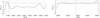 |
Fig. 7. Variation of luminosity Δℒ(t). The horizontal dashed line is ℒ0 (cf. Eq. (27)), whereas the vertical dashed line marks T0. The order of the sources is as in Fig. 3. |
4.1.2. Differences
The described similarities are mainly due to the underlying equal mathematical structure, while the discrepancies arise from the different physical nature of the two spider classes. Observationally, the orbits associated with 47 Tuc W appear to be tighter than those of 47 Tuc O (see Fig. 4). This trend is consistent with theoretical models of spider pulsars, which suggest that the pulsar wind significantly impacts the companion’s structure and mass-loss process (Chen et al. 2013; Wang et al. 2021; Conrad-Burton et al. 2023). The high-energy photons emitted by the pulsar deposit energy in the companion’s outer layers, altering its convection properties and potentially leading to enhanced material loss. While mass-loss rates in black widows and redbacks depend on multiple factors, including the intensity of irradiation and orbital evolution, models indicate that redback companions – which are more massive – may sustain a stronger magnetic field, which provides greater resistance to ablation-driven mass loss (Conrad-Burton et al. 2023).
The magnetic fields of redbacks exhibit larger fluctuations (with shifts of up to 150 kG) compared to the more stable 20 kG variations in black widows. However, the magnetic activity in redbacks is observed to persist for shorter timescales than in black widows (see Table A.1). This behaviour fits the irradiation-driven evolution scenario, where the pulsar’s relativistic wind and high-energy radiation interact with the companion’s magnetosphere (Conrad-Burton et al. 2023). In redbacks, the stronger magnetic field can counteract the pulsar wind for longer, delaying the complete stripping of the companion. In contrast, the weaker fields of black-widow companions result in a more effective removal of material, leading to more rapid and extreme ablation (Podsiadlowski 1991; Chen et al. 2013; Conrad-Burton et al. 2023). Interestingly, while ablation is commonly associated with more severe mass loss in black widows, it is expected that redbacks’ companions can intercept a larger fraction of the pulsar’s spin-down luminosity, possibly as a result of a different geometric configuration (Chen et al. 2013; Conrad-Burton et al. 2023). This effect likely stems from the more substantial convective envelope and deeper energy deposition in redback companions, which alters their thermal and magnetic structures.
From a modelling perspective, a convincing explanation of the connection between the directly observed surface and bulk magnetic-field properties of these systems is still missing. The the most advanced and relevant studies on this topic follow two distinct approaches, mainly based on three-dimensional MHD simulations (Browning 2008; Yadav et al. 2015; MacDonald & Mullan 2017) and one-dimensional stellar-evolution analyses (Feiden & Chaboyer 2014). We can see that in the aforementioned works there is an ongoing disagreement about the order of magnitude of the field intensity in fully convective stars: some authors require ∼MG fields, while others insist on possible upper limits of ∼10 kG. Given this lack of consensus, our 20–100 kG sub-surface field variation (see Fig. 6) at a depth of ∼0.1Rc (Applegate 1992a) seems to be reasonable. Currently, there are no simulations specifically focused on this aspect, and up to now there are only some indications that the sub-surface magnetic field could be larger than the surface one by a factor of ∼2 (see for details Fig. 4 in Yadav et al. 2015).
One of the novel aspects of our model with respect to the literature relies on the temporal dynamics of the ΔB(t) plot. The long-term evolution of the surface fields is sometimes observed, while the suggested drastic variation of the field intensity by a factor of ∼10 with a characteristic oscillatory shape seems to be absent from any other observations or theoretical modelling of fully convective stars outside spider systems. It is true that our profile is based on a rudimentary formula of the magnetic field, but the conventional dynamo models interplay with the quadrupole variations in these stars, possibly generating new behaviours.
Regarding luminosity, redback companions generally exhibit higher optical luminosities than black widows, as shown in Fig. 7. This trend arises from a combination of factors (Roberts 2012; Gentile et al. 2014; Roberts et al. 2018; Strader et al. 2019; Sullivan & Romani 2024): (i) the intrinsic luminosity of the star, which is modulated by pulsar heating; (ii) the pulsar wind interaction with the companion and the surrounding material, particularly in X-ray bands; (iii) the gamma-ray emission from pulsar magnetospheric processes such as curvature radiation and inverse Compton scattering; (iv) occasional mass-transfer episodes, where infalling matter is energised by the pulsar’s magnetic field; and (v) non-thermal radiation from the intra-binary shock formed between the pulsar wind and the ablated material.
In our case, redbacks reach total luminosities of ℒ0 ∼ 1035 erg/s, while black widows are typically a few orders of magnitude dimmer (ℒ0 ∼ 1031 erg/s). The larger companion star and stronger irradiation in redbacks contribute to a higher optical luminosity. However, in the X-ray and gamma-ray bands, black widows can still exhibit comparable or even greater luminosities due to the more efficient formation of intra-binary shocks (Conrad-Burton et al. 2023). These findings suggest that spider systems provide a unique laboratory for studying the effects of extreme irradiation on stellar magnetism, convection, and mass-loss processes. Future observational constraints and detailed simulations will be crucial to further refining our understanding of the evolution of these exotic binary systems.
4.2. Parameter determination
In the current study, it was of essential importance to understand how to determine the parameters associated with a spider system using our model, which is fully based on the Applegate mechanism. This process is critical for extracting detailed information about the gravitational source under investigation. Broadly speaking, two main approaches can be identified.
The first route relies on the fact that when a new spider source is discovered, we can generally fit the orbital period modulations, thus obtaining the parameters T0, the TEMPO coefficients {fi}I = 0n, and Pma. Now, assuming that the NS has a canonical mass of mp = 1.4 M⊙ and that the system is observed nearly edge-on, the mass of the companion star, mc, can then be estimated (see e.g., Ridolfi et al. 2016; Freire et al. 2017, for more details). This step is crucial to determine the spider system nature, namely whether it is a redback or a black widow. Subsequently, we can estimate the companion star’s radius, Rc, by adopting the same argument detailed in Appendix A. Using Kepler’s third law, the initial orbital separation, a, can then be calculated. By applying these criteria, we obtain a comprehensive measurement of all the independent parameters.
An alternative strategy shares with the above procedure the determination of the parameters T0, {fi}i = 0n, and Pma from the observations, while leaving the remaining four parameters mp, mc, Rc, a to be inferred. They could be potentially determined if we have experimental data pertaining to a physical observable, such as the luminosity profile (26), which encapsulates a combination of all these unknowns. By fitting such data and extracting the best-fit parameters, with the annex constraints on the variation ranges and the validity of Kepler’s third law, a consistent set of values can be extracted. Depending on the available data, one or the other strategy could be used. Obviously, the available data vary from system to system.
5. Conclusions
This article deals with spider binary systems, which are formed by a pulsar and a low-mass companion star, classified as redbacks (mc ∼ 0.1 − 0.4 M⊙) and black widows (mc ≪ 0.1 M⊙). One of their distinctive features on which we concentrated is the long-term unpredictable variations in the orbital period and its first derivative (Roberts et al. 2014). Among the different contributions, which can account for orbital period modulations, it has been clearly shown that the most reasonable explanation is due to the Applegate mechanism (Applegate & Patterson 1987; Applegate 1992a,b). This description accounts for orbital-timing variations via the companion star’s quadrupole-moment changes induced by the magnetic dynamo action, which in turn is communicated to the orbital motion through quadrupole-gravity coupling.
This work constitutes the first attempt to make the Applegate mechanism dynamical. To the best of our knowledge, we provide the spider observables’ evolution for the first time. Combining information derived by pulsar-timing observations and assuming the Applegate mechanism as true, we were able to track the evolution in time (within a determined timeframe) of some physical quantities (see Eq. (33)).
Voisin et al. (2020a,b) considerably improved the treatment of the quadrupole deformations while also adding relativistic effects, but they only provided the dynamical evolution of the quadrupole moment. Another important difference between Voisin et al. (2020a,b) and our approach lies in the final goals. Voisin et al. (2020a,b) proposed a detailed model for describing the motion of spider binary systems to accurately estimate the observed ΔP variations with the ultimate objective of improving the timing solution pertaining to these gravitational sources.
On the other side, our work employs a reverse approach: rather than finding a physical justification for the ΔP variations, we take them from the long-term observations and, by relying on the validity of the Applegate mechanism, we reconstruct the dynamics of the related physical variables. Therefore, we follow an observational and deductive analysis instead of a theoretical and inductive one. Even though our model is very simple, we emphasise that it could also be applied to more refined frameworks.
To achieve our goal, we first derived the equations of motion (10)–(14) pertaining to the dynamics of spider binaries, based on the Applegate works. Then, we considered the function ΔP(t), reconstructed by fitting the observational data on the orbital period modulations. However, the resolution of this problem can most likely only be accomplished numerically, and this can be excessively time consuming. To this end, we developed a mathematical procedure (see Sect. 3) based on approximating the quasi-circular orbit with a circular one, even though it presents mild oscillations on small timescales. This strategy allowed us to obtain rS(t) without solving Eq. (10). Substituting this function and ΔP(t) into Eq. (14), we obtain that the ensuing differential equation is still difficult to solve analytically.
Therefore, to avoid any kind of numerical integration, we approximated rS(t) and ΔP(t) with highly accurate polynomials. This allowed us to have an analytical expression of Q(t), whose functional formula is reported in Eq. (31). This result is in good agreement with the corresponding function computed by numerically integrating Eqs. (10)–(14) together, without making any simplifying hypothesis. Through these formulae, it has been possible to easily obtain the evolution of the related physical observables, which are (see Sect. 2.4) orbits, quadrupole moment, magnetic field, and luminosity.
In Fig. 3, we display the orbital-period modulations of the redback 47 Tuc W and black widow 47 Tuc O, whereas in Figs. 4, 5, 6, and 7 we show the evolution of the related physical observables via our model. We discussed analogies and differences between the two sources (see Sect. 4.1), which are representatives of the redbacks and black widows. We contextualised these results in a more general physical picture.
The advantages of our approach are (1) the use of simple formulae; (2) having the evolution of the above-described physical variables, which make it possible to better model through future upgraded descriptions; (3) having insight into the sub-surface magnetic activity inside the companion star, which is still not a clear topic; (4) employing our analytical formulae to tightly constrain the model parameters by using not only the orbital period modulations, but also the profiles of other observables (used the luminosity profile as further information, e.g. Zhao & Heinke 2023); and (5) the vast application of our developments to more updated or different descriptions of spider binary systems. However, our treatment possesses some evident limits: (1) the model is very simple and must be improved under different rudimentary aspects; (2) the magnetic field necessitates modelling through more realistic formulae – based on MHD simulations (Dobler et al. 2006; Browning 2008) – to clarify the link between surface and sub-surface magnetic fields, which are still not fully treated (Morin 2012); (3) it is not adequate to reproduce dissipative phenomena (Lanza 2006) or new effects such as the general-relativistic corrections and the three-dimensional motion of the two bodies (Voisin et al. 2020a,b); and (4) the model prediction power is limited only within the observational period [t0, t1].
Future perspectives can cover several routes. First, the methodology and results of this article could be applied to catalogue all the available spider systems and to perform more accurate analyses in order to extract relevant information on stellar evolution and to classify the pulsar population in a more methodical fashion. Another possible development is to derive a more useful equation from actual MHD simulations to better model the magnetic activity inside the companion star.
See https://www.atnf.csiro.au/research/pulsar/psrcat for more details. However, the situation is as follows: within the galactic plane, 135 are isolated and 209 are binaries; whereas in globular clusters, 87 are isolated and 91 are binaries.
In this investigation, three aspects had to be considered: (1) the mass loss from the companion amounting to 10−10 M⊙/yr (Pan et al. 2023); (2) the fact that if the Roche lobe is smaller than the radius of the companion star, there is mass transfer; and (3) the pulsar wind entailing a mass loss of 10−12 M⊙/yr (Guerra et al. 2024). We conclude that we can consider constant mass.
The companion star’s variations are due to the combination of two effects: quadrupole changes amounting to 1 − 5% (Applegate 1992a; Harvey et al. 1995), and magnetic-field dynamo activity causing fluctuations of 2 − 6% (Rappaport et al. 1983; MacDonald & Mullan 2009). The combined effects can thus range from 5 − 7%.
The quadrupole moment is a tensor written in terms of the companion star’s inertial tensor. In our hypotheses, we have Q = Qxx (see for details discussion under Eq. (3) in Applegate 1992a).
We preferred to work in normalised units to develop the calculations since this is advantageous during the fitting procedure.
For circular orbits, T0 is the ascending node’s epoch passage.
It is important to note that with Q being directed along the x-axis, thanks to the transformation (1), we obtain that Q(t) points along rS(t).
It is important to note that ΔP(t) = P(t)−P0, with P0 being a constant. Therefore, dΔP/dt = Ṗ(t). We use both notations in this paper.
Acknowledgments
The authors greatly thank Oleg Kochukhov for valuable comments on our results. V.D.F. is grateful to Gruppo Nazionale di Fisica Matematica of Istituto Nazionale di Alta Matematica (INDAM) for support. V.D.F. acknowledges the support of INFN sez. di Napoli, iniziativa specifica TEONGRAV. V.D.F. is grateful to both the SRT – Sardinia Radio Telescope and the Max Planck Institute für Radioastronomie in Bonn for the hospitality. A.Ca. is grateful to Scuola Superiore Meridionale for hospitality. A.R. is supported by the Italian National Institute for Astrophysics (INAF) through an ‘IAF – Astrophysics Fellowship in Italy’ fellowship (Codice Unico di Progetto: C59J21034720001; Project ‘MINERS’). AR also acknowledges continuing valuable support from the Max-Planck Society.
References
- Alpar, M. A., Cheng, A. F., Ruderman, M. A., & Shaham, J. 1982, Nature, 300, 728 [NASA ADS] [CrossRef] [Google Scholar]
- Applegate, J. H. 1992a, ApJ, 385, 621 [Google Scholar]
- Applegate, J. H. 1992b, in Cool Stars, Stellar Systems, and the Sun, eds. M. S. Giampapa, & J. A. Bookbinder, ASP Conf. Ser., 26, 343 [Google Scholar]
- Applegate, J. H., & Patterson, J. 1987, ApJ, 322, L99 [NASA ADS] [CrossRef] [Google Scholar]
- Applegate, J. H., & Shaham, J. 1994, ApJ, 436, 312 [NASA ADS] [CrossRef] [Google Scholar]
- Balbus, S. A., & Brecher, K. 1976, ApJ, 203, 202 [Google Scholar]
- Baliunas, S. L., & Vaughan, A. H. 1985, ARA&A, 23, 379 [NASA ADS] [CrossRef] [Google Scholar]
- Belczynski, K., Lorimer, D. R., Ridley, J. P., & Curran, S. J. 2010, MNRAS, 407, 1245 [Google Scholar]
- Bhattacharya, D., & van den Heuvel, E. P. J. 1991, Phys. Rep., 203, 1 [Google Scholar]
- Bisnovatyi-Kogan, G. S., & Komberg, B. V. 1974, Sov. Ast., 18, 217 [Google Scholar]
- Blandford, R., & Teukolsky, S. A. 1976, ApJ, 205, 580 [Google Scholar]
- Bochenek, C., Ransom, S., & Demorest, P. 2015, ApJ, 813, L4 [NASA ADS] [Google Scholar]
- Bogdanov, S., Grindlay, J. E., & van den Berg, M. 2005, ApJ, 630, 1029 [Google Scholar]
- Bogovalov, S. V., Khangulyan, D. V., Koldoba, A. V., Ustyugova, G. V., & Aharonian, F. A. 2008, MNRAS, 387, 63 [Google Scholar]
- Bogovalov, S. V., Khangulyan, D., Koldoba, A. V., Ustyugova, G. V., & Aharonian, F. A. 2012, MNRAS, 419, 3426 [NASA ADS] [CrossRef] [Google Scholar]
- Bours, M. C. P., Marsh, T. R., Parsons, S. G., et al. 2016, MNRAS, 460, 3873 [Google Scholar]
- Browning, M. K. 2008, ApJ, 676, 1262 [Google Scholar]
- Browning, M. K., Miesch, M. S., Brun, A. S., & Toomre, J. 2006, ApJ, 648, L157 [Google Scholar]
- Chandrasekhar, S. 1961, Hydrodynamic and hydromagnetic stability [Google Scholar]
- Charbonneau, P., & Dikpati, M. 2000, ApJ, 543, 1027 [NASA ADS] [CrossRef] [Google Scholar]
- Chen, H.-L., Chen, X., Tauris, T. M., & Han, Z. 2013, ApJ, 775, 27 [NASA ADS] [CrossRef] [Google Scholar]
- Choudhuri, A. R., Schussler, M., & Dikpati, M. 1995, A&A, 303, L29 [NASA ADS] [Google Scholar]
- Conrad-Burton, J., Shabi, A., & Ginzburg, S. 2023, MNRAS, 525, 2708 [NASA ADS] [Google Scholar]
- D’Antona, F., & Ergma, E. 1993, A&A, 269, 219 [Google Scholar]
- Demory, B. O., Ségransan, D., Forveille, T., et al. 2009, A&A, 505, 205 [NASA ADS] [CrossRef] [EDP Sciences] [Google Scholar]
- Dobler, W., Stix, M., & Brandenburg, A. 2006, ApJ, 638, 336 [NASA ADS] [CrossRef] [Google Scholar]
- Donati, J.-F., Collier Cameron, A., Semel, M., et al. 2003, MNRAS, 345, 1145 [NASA ADS] [CrossRef] [Google Scholar]
- Dormand, J., & Prince, P. 1980, J. Comput. Appl. Math., 6, 19 [CrossRef] [MathSciNet] [Google Scholar]
- Falanga, M., Kuiper, L., Poutanen, J., et al. 2005, A&A, 444, 15 [NASA ADS] [CrossRef] [EDP Sciences] [Google Scholar]
- Feiden, G. A., & Chaboyer, B. 2014, ApJ, 789, 53 [NASA ADS] [CrossRef] [Google Scholar]
- Frank, J., King, A., & Raine, D. J. 2002, Accretion Power in Astrophysics (Third Edition), 398 [Google Scholar]
- Freire, P. C. C., Ridolfi, A., Kramer, M., et al. 2017, MNRAS, 471, 857 [Google Scholar]
- Fruchter, A. S., Stinebring, D. R., & Taylor, J. H. 1988, Nature, 333, 237 [Google Scholar]
- Gentile, P. A., Roberts, M. S. E., McLaughlin, M. A., et al. 2014, ApJ, 783, 69 [NASA ADS] [CrossRef] [Google Scholar]
- Guerra, C., Meliani, Z., & Voisin, G. 2024, A&A, 690, A75 [NASA ADS] [CrossRef] [EDP Sciences] [Google Scholar]
- Hall, D. S. 1990, NATO Adv. Sci. Inst. (ASI) Ser. C, 319, 95 [Google Scholar]
- Han, E., Lopez-Valdivia, R., Mace, G., & Jaffe, D. 2023, Am. Astron. Soc. Meeting Abstr., 241, 42907 [Google Scholar]
- Harvey, D., Skillman, D. R., Patterson, J., & Ringwald, F. A. 1995, PASP, 107, 551 [Google Scholar]
- Kaplan, D. L., Bhalerao, V. B., van Kerkwijk, M. H., et al. 2013, ApJ, 765, 158 [NASA ADS] [CrossRef] [Google Scholar]
- Kluzniak, W., Ruderman, M., Shaham, J., & Tavani, M. 1988, Nature, 334, 225 [NASA ADS] [CrossRef] [Google Scholar]
- Kochanek, C. S. 1992, ApJ, 385, 604 [NASA ADS] [CrossRef] [Google Scholar]
- Lanza, A. F. 2006, MNRAS, 369, 1773 [NASA ADS] [CrossRef] [Google Scholar]
- Lanza, A. F., & Rodonò, M. 1999, A&A, 349, 887 [Google Scholar]
- Lanza, A. F., & Rodonò, M. 2002, Astron. Nachr., 323, 424 [NASA ADS] [CrossRef] [Google Scholar]
- Lanza, A. F., Rodono, M., & Rosner, R. 1998, MNRAS, 296, 893 [Google Scholar]
- Lazaridis, K., Verbiest, J. P. W., Tauris, T. M., et al. 2011, MNRAS, 414, 3134 [CrossRef] [Google Scholar]
- MacDonald, J., & Mullan, D. J. 2009, ApJ, 700, 387 [Google Scholar]
- MacDonald, J., & Mullan, D. J. 2017, ApJ, 850, 58 [NASA ADS] [CrossRef] [Google Scholar]
- Morin, J. 2012, EAS Publ. Ser., 57, 165 [Google Scholar]
- Ng, C. W., Takata, J., Strader, J., Li, K. L., & Cheng, K. S. 2018, ApJ, 867, 90 [NASA ADS] [Google Scholar]
- Pallanca, C., Mignani, R. P., Dalessandro, E., et al. 2012, ApJ, 755, 180 [NASA ADS] [CrossRef] [Google Scholar]
- Pan, Z., Lu, J. G., Jiang, P., et al. 2023, Nature, 620, 961 [CrossRef] [Google Scholar]
- Papitto, A., Ferrigno, C., Bozzo, E., et al. 2013, Nature, 501, 517 [NASA ADS] [CrossRef] [Google Scholar]
- Parker, E. N. 1955, ApJ, 122, 293 [Google Scholar]
- Parker, E. N. 1979, ApJ, 230, 905 [Google Scholar]
- Podsiadlowski, P. 1991, Nature, 350, 136 [CrossRef] [Google Scholar]
- Press, W. H., Teukolsky, S. A., Vetterling, W. T., & Flannery, B. P. 2002, Numerical recipes in C++ : the art of scientific computing [Google Scholar]
- Radhakrishnan, V., & Srinivasan, G. 1982, Curr. Sci., 51, 1096 [NASA ADS] [Google Scholar]
- Rappaport, S., Verbunt, F., & Joss, P. C. 1983, ApJ, 275, 713 [Google Scholar]
- Rasio, F. A., Shapiro, S. L., & Teukolsky, S. A. 1989, ApJ, 342, 934 [Google Scholar]
- Ridolfi, A., Freire, P. C. C., Torne, P., et al. 2016, MNRAS, 462, 2918 [Google Scholar]
- Roberts, M. S. E. 2012, Proc. Int. Astron. Union, 8, 127 [CrossRef] [Google Scholar]
- Roberts, M. S. E. 2013, in Neutron Stars and Pulsars: Challenges and Opportunities after 80 years, ed. J. van Leeuwen, IAU Symp., 291, 127 [Google Scholar]
- Roberts, M. S. E., Mclaughlin, M. A., Gentile, P., et al. 2014, Astron. Nachr., 335, 313 [Google Scholar]
- Roberts, M. S. E., Al Noori, H., Torres, R. A., et al. 2018, in Pulsar Astrophysics the Next Fifty Years, eds. P. Weltevrede, B. B. P. Perera, L. L. Preston, & S. Sanidas, IAU Symp., 337, 43 [Google Scholar]
- Romani, R. W., Filippenko, A. V., Silverman, J. M., et al. 2012, ApJ, 760, L36 [NASA ADS] [CrossRef] [Google Scholar]
- Ruderman, M., Shaham, J., Tavani, M., & Eichler, D. 1989, ApJ, 343, 292 [NASA ADS] [CrossRef] [Google Scholar]
- Shaifullah, G., Verbiest, J. P. W., Freire, P. C. C., et al. 2016, MNRAS, 462, 1029 [Google Scholar]
- Smedley, S. L., Tout, C. A., Ferrario, L., & Wickramasinghe, D. T. 2015, MNRAS, 446, 2540 [Google Scholar]
- Sorahana, S., Yamamura, I., & Murakami, H. 2013, ApJ, 767, 77 [NASA ADS] [CrossRef] [Google Scholar]
- Stappers, B. W., Bailes, M., Lyne, A. G., et al. 1996a, ApJ, 465, L119 [NASA ADS] [CrossRef] [Google Scholar]
- Stappers, B. W., Bessell, M. S., & Bailes, M. 1996b, ApJ, 473, L119 [NASA ADS] [CrossRef] [Google Scholar]
- Stappers, B. W., Bailes, M., Lyne, A. G., et al. 2001, MNRAS, 321, 576 [NASA ADS] [Google Scholar]
- Stappers, B. W., Archibald, A. M., Hessels, J. W. T., et al. 2014, ApJ, 790, 39 [Google Scholar]
- Sterne, T. E. 1939, MNRAS, 99, 451 [NASA ADS] [Google Scholar]
- Strader, J., Swihart, S., Chomiuk, L., et al. 2019, ApJ, 872, 42 [Google Scholar]
- Sullivan, A. G., & Romani, R. W. 2024, ApJ, 974, 315 [NASA ADS] [Google Scholar]
- van Buren, D. 1986, AJ, 92, 136 [NASA ADS] [Google Scholar]
- van den Heuvel, E. P. J., & van Paradijs, J. 1988, Nature, 334, 227 [NASA ADS] [CrossRef] [Google Scholar]
- Voisin, G., Breton, R. P., & Summers, C. 2020a, MNRAS, 492, 1550 [NASA ADS] [CrossRef] [Google Scholar]
- Voisin, G., Clark, C. J., Breton, R. P., et al. 2020b, MNRAS, 494, 4448 [Google Scholar]
- Wang, S. Q., Wang, J. B., Wang, N., et al. 2021, ApJL, 922, L13 [Google Scholar]
- Warner, B. 1988, Nature, 336, 129 [NASA ADS] [CrossRef] [Google Scholar]
- Wijnands, R., & van der Klis, M. 1998, Nature, 394, 344 [CrossRef] [Google Scholar]
- Yadav, R. K., Christensen, U. R., Morin, J., et al. 2015, ApJ, 813, L31 [Google Scholar]
- Yoshida, S. 2019, MNRAS, 486, 2982 [NASA ADS] [CrossRef] [Google Scholar]
- Zahn, J. P. 2008, EAS Publ. Ser., 29, 67 [NASA ADS] [CrossRef] [EDP Sciences] [Google Scholar]
- Zhao, J., & Heinke, C. O. 2023, MNRAS, 526, 2736 [NASA ADS] [CrossRef] [Google Scholar]
Appendix A: Polynomial approximations
We provide the polynomial approximations of ΔP(t),rS(t),Q(t) with the related MRE for the spider systems 47 Tuc W (see Eq. (A.1)) and 47 Tuc O (see Eq. (A.2)). The input parameters of these two physical systems are reported in Table A.1.
We assume that the pulsar mass is the standard value mp = 1.4M⊙. The companion star’s mass, mc is taken from works cited in the caption of Table A.1, assuming that the binary system is seen by the observer almost edge on, namely sin i = 1 with i inclination of the observer with respect to the z-axis. Instead, the initial binary separation a is calculated via the Kepler’s third law (cf. Eq. (18)), employing f0 = 1/P0, mp, mc.
Regarding the companion star’s radius (at rest), Rc, there is no guidance on its calculation in the referenced papers on the two sources. To estimate it, we follow this strategy. In black widows, the companion can reach extremely low masses, as seen in 47 Tuc O, suggesting it may be a brown dwarf, whose radius typically falls within the range 0.064 − 0.113R⊙ (Sorahana et al. 2013). For our purposes, we adopt an average radius of Rc = 0.08R⊙. In contrast, for redbacks, the companion is a main-sequence star, allowing us to estimate its radius using the following formula (see Table A.1 and Demory et al. 2009):
 (A.1)
(A.1)
The radii we have selected are in agreement with the Roche lobe size RL of the two sources (Frank et al. 2002), as for 47 TUC W we have Rc/RL = 0.78, while for 47 TUC O it is Rc/RL = 0.63.
We show the input parameters (32) pertaining to 47 Tuc W and 47 Tuc O, as well as the quantities Q0 (cf. Eq. (15)), B0 (cf. Eq. (23)), and ℒ0 (cf. Eq. (27)). We express all masses and distances in terms of the solar mass M⊙ = 2 × 1033g and the solar radius R⊙ = 6.96 × 1010cm, respectively. The input parameters and TEMPO coefficients t0, t1, T0, {fi}i = 0n are both taken from Ridolfi et al. (2016), Freire et al. (2017). For more details on how a and Rc have been calculated/chosen, we refer to the beginning of Appendix A.
A.1. Redback: 47 Tuc W
We approximate ΔP(t) with the polynomial
 (A.2)
(A.2)
where t ∈ [0, 1], which can be cast in [t0, t1] via Eq. (6), and 𝒫1(t) has the dimension of ms. The related MRE is ∼10−5%, which is extremely accurate, since we have used a ninth-order polynomial (see discussion of Sec. 3.1, for details).
We use the approximation (A.2) for calculating the radius rS(t) (cf. Eqs. (29) and (30)), committing a MRE of ∼10−13%, which is still very accurate. For the quadrupole moment, we employ Eq. (11) and this polynomial approximation for rS(t)
 (A.3)
(A.3)
where t ∈ [0, 1] and ℛ1(t) is expressed in cm. The MRE for rS(t) is of ∼10−13%. Using this approach, the MRE on Q(t) is ∼ × 10−3%, which is still in good agreement. We conclude that the quadrupole moment is approximated with respect to the original solution with a MRE of 0.004%.
A.2. Black widow: 47 Tuc O
We approximate ΔP(t) with the polynomial (in ms unit)
 (A.4)
(A.4)
where t ∈ [0, 1], whose related MRE is ∼ × 10−3%, being very accurate, as 𝒫2(t) is of twelfth order (see Sec. 3.1, for details).
The approximation (A.4) is exploited for computing the radius rS(t) with a MRE of ∼10−14%. The estimation of the quadrupole moment (11) is performed by approximating the radius rS(t) via the following polynomial (in cm unit and t ∈ [0, 1])
 (A.5)
(A.5)
The associated MRE is of ∼10−12%. Therefore, the MRE on Q(t) is ∼10−4%, being in perfect agreement with the original formula. Finally, the quadrupole moment is approximated with respect to the original solution with a MRE of 0.03%.
All Tables
We show the input parameters (32) pertaining to 47 Tuc W and 47 Tuc O, as well as the quantities Q0 (cf. Eq. (15)), B0 (cf. Eq. (23)), and ℒ0 (cf. Eq. (27)). We express all masses and distances in terms of the solar mass M⊙ = 2 × 1033g and the solar radius R⊙ = 6.96 × 1010cm, respectively. The input parameters and TEMPO coefficients t0, t1, T0, {fi}i = 0n are both taken from Ridolfi et al. (2016), Freire et al. (2017). For more details on how a and Rc have been calculated/chosen, we refer to the beginning of Appendix A.
All Figures
|
Fig. 1. Illustration of typical spider binary system. An MSP and a companion star are in a tidally locked configuration, moving in synchronous rotations on quasi-circular and tight orbits. They are separated by a distance of rs(t) in a plane orthogonal to the orbital angular-momentum vector L, which is conserved during the binary system’s motion. The irradiation-driven wind from the MSP heats through a tidal dissipation the companion star, which starts to evaporate, thus losing mass. This is the eclipsing material, which acts as an obstacle to the radio signal detected by a telescope located far from the binary system. In the dashed red box we sketch the companion star’s interior. This zone is characterised by a convective envelope, where the fluid in it is highly conductive. Furthermore, the pulsar wind triggers the differential rotation of the companion star, which induces a magnetic activity through a dynamo action. The subsurface magnetic field is responsible for breaking the hydrostatic equilibrium inside the star, inducing quadrupole moment changes. We note that the external magnetic field is expected to be locally poloidal, while the sub-surface field is toroidal. |
| In the text | |
|
Fig. 2. We display two RFs: ℛCO (black) and ℛS (red). |
| In the text | |
|
Fig. 3. Orbital-period modulations of 47 Tuc W and 47 Tuc O, obtained from the fitting of the observational data (see Table A.1). The vertical dashed line marks the position of T0. |
| In the text | |
|
Fig. 4. Discrepancy of actual separation among the bodies with respect to the initial datum. The vertical dashed line marks T0. The order of the sources is placed as in Fig. 3. |
| In the text | |
|
Fig. 5. Evolution of quadrupole moment Q(t)/Q0, where the horizontal dashed line is set at 1 and the vertical dashed line marks T0. The order of the sources is as in Fig. 3. |
| In the text | |
|
Fig. 6. Variation of magnetic-field intensity ΔB(t). The horizontal dashed line is B0 (cf. Eq. (23)), whereas the vertical dashed line marks T0. The order of the sources is as in Fig. 3. |
| In the text | |
|
Fig. 7. Variation of luminosity Δℒ(t). The horizontal dashed line is ℒ0 (cf. Eq. (27)), whereas the vertical dashed line marks T0. The order of the sources is as in Fig. 3. |
| In the text | |
Current usage metrics show cumulative count of Article Views (full-text article views including HTML views, PDF and ePub downloads, according to the available data) and Abstracts Views on Vision4Press platform.
Data correspond to usage on the plateform after 2015. The current usage metrics is available 48-96 hours after online publication and is updated daily on week days.
Initial download of the metrics may take a while.