| Issue |
A&A
Volume 620, December 2018
|
|
|---|---|---|
| Article Number | A167 | |
| Number of page(s) | 11 | |
| Section | Planets and planetary systems | |
| DOI | https://doi.org/10.1051/0004-6361/201833227 | |
| Published online | 11 December 2018 | |
Toward understanding the origin of asteroid geometries
Variety in shapes produced by equal-mass impacts
Department of Physics, Nagoya University,
Aichi 464-8602, Japan
e-mail: sugiura.keisuke@a.mbox.nagoya-u.ac.jp
Received:
13
April
2018
Accepted:
9
October
2018
More than a half of the asteroids in the main belt have irregular shapes with ratios of the minor to major axis lengths of less than 0.6. One of the mechanisms that create such shapes is collisions between asteroids. The relationship between the shapes of collisional outcomes and impact conditions such as impact velocities may provide information on the collisional environments and its evolutionary stages when those asteroids are created. In this study, we perform numerical simulations of collisional destruction of asteroids with radii 50 km and subsequent gravitational reaccumulation using smoothed-particle hydrodynamics for elastic dynamics with self-gravity, a model of rock fractures, and a model of friction in completely damaged rock. We systematically vary the impact velocity from 50 to 400 m s−1 and the impact angle from 5° to 45°. We investigate shapes of the largest remnants resulting from collisional simulations. As a result, various shapes (bilobed, spherical, flat, elongated, and hemispherical shapes) are formed through equal-mass and low-velocity (50−400 m s−1) impacts. We clarify a range of the impact angle and velocity to form each shape. Our results indicate that irregular shapes, especially flat shapes, of asteroids with diameters larger than 80 km are likely to be formed through similar-mass and low-velocity impacts, which are likely to occur in the primordial environment prior to the formation of Jupiter.
Key words: minor planets, asteroids: general / methods: numerical
© ESO 2018
1 Introduction
Planets are formed in protoplanetary disks around protostars through collisional coalescence of planetesimals (Safronov 1969; Hayashi et al. 1985). The growth mode of planetesimals is considered to be runaway; that is, larger planetesimals grow more rapidly than smaller ones (e.g., Greenberg et al. 1978; Wetherill & Stewart 1989; Kokubo & Ida 1996). The runaway growth produces a bimodal mass distribution of bodies composed of protoplanets and remnant planetesimals of mass around the onset of runaway growth (Kobayashi et al. 2016). Main-belt asteroids located between the orbits of Mars and Jupiter may be remnants of planetesimals (e.g., Petit et al. 2001; Bottke et al. 2005). A large number of asteroids (more than 100 000 asteroids with diameters >1 km) allows statistical discussion to reveal the history of the solar system.
Asteroids have a variety of shapes. Recent in situ observations by spacecraft and light curve and radar observations by ground-based telescopes reveal the shapes of about 1000 asteroids. Those obtained from light curves are summarized in the Database of Asteroid Models from Inversion Techniques (DAMIT; Ďurech et al. 2010). According to asteroidal shapes obtained from various observations, the shapes of many asteroids smaller than 100 km are distinctly different from planet shapes, which are almost spheres (Fujiwara et al. 2006; Ďurech et al. 2010; Marchis et al. 2014; Cibulková et al. 2016). Some asteroids with diameters larger than 100 km also have irregular shapes. For example, (624) Hektor has a very elongated shape with an intermediate axis length of 195 km and major axis length of 370 km (Storrs et al. 1999). In this paper, we define irregular shapes as shapes with axis ratios of less than 0.6.
Asteroids with irregular shapes may be formed through collisional destruction of planetesimals. The formation of irregular shapes of rubble piles through collisional destruction of planetesimals and gravitational reaccumulation is investigated using the smoothed-particle hydrodynamics (SPH) method or N-body code with models of material strength. Some impact simulations reproduce the formation of elongated shapes like (25143) Itokawa or bilobed shapes like 67P/Churyumov–Gerasimenko (Michel & Richardson 2013; Jutzi & Asphaug 2015; Jutzi & Benz 2017; Schwartz et al. 2018).
Shapes of objects formed through collisional destruction or coalescence depend on impact conditions (e.g., Jutzi & Asphaug 2015). For example, collisions with impact velocities comparable to the escape velocity result in simple merging. In contrast, collisions with higher impact velocities result in catastrophic destruction, and shapes are determined through the gravitational reaccumulation of fragments. Thus, the relationship between the impact conditions and the resultant shapes clarifies the impact conditions (e.g., impact velocities) that form irregular shapes of asteroids and then gives constraints on the collisional environment (e.g., eccentricity distribution) that forms asteroids.
Collisional lifetimes of asteroids with diameters ≳10 km in the present main belt are estimated to be ~10 Gyr, which is greater than the age of the solar system (O’Brien & Greenberg 2005). Although collisional destruction of asteroids with diameters ≳10 km in the present solar system is rare, destructive collisions are expected to be more frequent in the primordial environment because the formation and migration of Jupiter may significantly deplete asteroids (Bottke et al. 2005; Walsh et al. 2011). Thus, the shapes of large asteroids may preserve those formed in the primordial solar system. In the planet formation era, eccentricities of planetesimals are small around young planets with small masses (e.g., Wetherill & Stewart 1993; Kokubo & Ida 1998; Inaba et al. 2003; Kobayashi & Tanaka 2018), and impact velocities between young asteroids may be < 1 km s−1 because of the absence of large perturbers. Therefore, investigations of shapes formed through impacts with low impact velocities may suggestwhen asteroidal shapes were formed (e.g., prior to or after Jupiter formation).
In this study, we perform impact simulations to investigate collisional destruction of planetesimals and subsequent gravitational reaccumulation using the SPH method. For impacts with low impact velocities, the collisions that change shapes most efficiently are expected to be equal-mass impacts because impacts with high mass ratios tend to result in partial deformation, such as the formation of craters rather than catastrophic destruction. DAMIT already includes irregular shapes of ~ 200 asteroids with radii of~50 km. Therefore, we consider collisions between two planetesimals each with a radius of 50 km, and we focus on the dependence of resultant shapes on the impact velocity and angle.
The structure of this paper is as follows. In Sect. 2 we introduce SPH method and models for realistic rocky material. In Sect. 3 we describe initial conditions of impact simulations and the way to analyze results. Detailed results are introduced in Sect. 4, and in Sect. 5 we discuss the physical explanation for our results and application. In Sect. 6 we summarize our findings.
2 Method
2.1 SPH method
To investigate planetesimal collisions, we use the SPH method for elastic dynamics (Libersky & Petschek 1991). The SPH method is a computational fluid dynamics method utilizing Lagrangian particles (Monaghan 1992). In the framework of this method, we represent continuum material such as rock by using a cluster of particles. The motion of each particle is described by the equation of motion. Each particle has physical quantities such as density and internal energy, and these physical quantities are calculated from time evolution equations such as the equation of energy.
In order to treat elastic bodies by the SPH method, we use the following forms of basic equations1:
![\begin{align} &\frac{\textrm{d}\rho_{i}}{\textrm{d}t}=-\sum_{j}m_{j}\frac{\rho_{i}}{\rho_{j}}\left(v_{j}^{\alpha}-v_{i}^{\alpha}\right)\frac{\partial}{{\partial} x_{i}^{\alpha}}W(|\bm{x}_{i}-\bm{x}_{j}|,h),\\* &\frac{\textrm{d}v_{i}^{\alpha}}{\textrm{d}t}=\sum_{j}m_{j}\left[\frac{\sigma_{i}^{\alpha \beta}}{\rho_{i}^{2}} + \frac{\sigma_{j}^{\alpha \beta}}{\rho_{j}^{2}} - \Pi_{ij}\delta^{\alpha \beta} \right] \frac{\partial}{\partial x_{i}^{\beta}}W(|\bm{x}_{i}-\bm{x}_{j}|,h) + \sum_{j}g_{ij}^{\alpha},\end{align}](/articles/aa/full_html/2018/12/aa33227-18/aa33227-18-eq1.png)
![\begin{align*} &\frac{\textrm{d}u_{i}}{\textrm{d}t}= - \sum_{j}\frac{1}{2}m_{j}\left[\frac{p_{i}}{\rho_{i}^{2}} + \frac{p_{j}}{\rho_{j}^{2}} + \Pi_{ij} \right]\left(v_{j}^{\alpha}-v_{i}^{\alpha}\right)\frac{\partial}{\partial x_{i}^{\alpha}}W(|\bm{x}_{i}-\bm{x}_{j}|,h) \nonumber \\* & \, \ \ \ \ \ \ \ \ \ \ + \!\sum_{j}\!\frac{1}{2}m_{j}\frac{S_{i}^{\alpha \beta}}{\rho_{i}\rho_{j}} \left[\left(v_{j}^{\alpha}-v_{i}^{\alpha}\right)\frac{\partial}{\partial x_{i}^{\beta}} + \left(v_{j}^{\beta}-v_{i}^{\beta}\right)\frac{\partial}{\partial x_{i}^{\alpha}} \right] \!W(|\bm{x}_{i}-\bm{x}_{j}|,h).\end{align*}](/articles/aa/full_html/2018/12/aa33227-18/aa33227-18-eq2.png) (3)
(3)
Here, mi is the mass of the ith SPH particle, ρi is its density, vi is its velocity vector, xi is its position vector, h is a smoothing length,  is its stress tensor, ui is its specific internal energy, pi is its pressure,
  is its deviatoric stress tensor, δαβ is the Kronecker delta, W(r, h) is a kernel function, Πij is artificial viscosity, and gij is the gravity between the ith and jth particles. Superscripts in Greek letters mean a direction or component of a vector or tensor, and subscripts in Roman letters mean the particle number. We apply the summation rule over repeated indices in Greek letters. Using the pressure pi and the deviatoric stress tensor
  , the stress tensor
  is represented as
 (4)
(4)
For the kernel function, we use a Gaussian kernel given by
![\begin{equation*} W(r,h)=\left[\frac{1}{h\sqrt{\pi}} \right]^{3}\exp \left(-\frac{r^{2}}{h^{2}} \right).\end{equation*}](/articles/aa/full_html/2018/12/aa33227-18/aa33227-18-eq8.png) (5)
(5)
We set the smoothing length to be constant because of insignificant density variation. The smoothing length is determined by initial average particle spacing. The artificial viscosity is represented as
 (6)
(6)
Here, αvis and βvis are parameters for the artificial viscosity. We adopt αvis = 1.0 and βvis = 2.0. According to the kernel function, the gravity between the ith and jth particles is calculated as
 (7)
(7)
where G is the gravitational constant. According to Hooke’s law, deviatoric stress is proportional to strain. We calculate the time evolution of strain and then obtain the time evolution of deviatoric stress. The time evolution equation for the deviatoric stress tensor is given by
 (8)
(8)
where μ is the shear modulus;  and
and  are a strain rate tensor and a rotational rate tensor, respectively, and are represented as

We note that  and
and  are described by sums of velocity gradients. To treat rigid body rotation correctly, we adopt equations of velocity gradients with the correction matrix Li developed by Bonet & Lok (1999):
 (11)
(11)
For the equation of state, we use the Tillotson EoS (Tillotson 1962), which is often used for numerical simulations of impacts with the SPH method (e.g., Genda et al. 2012; Benz & Asphaug 1999). The Tillotson EoS has ten material dependent parameters. We assume a material of colliding planetesimals as basalt. Thus, we use values of the shear modulus and the Tillotson parameters for basalt described in Benz & Asphaug (1999).
For time integration, we use a leapfrog method with a kick-drift-kick scheme. Here, we use leapfrog equations with a form where the position and other physical quantities such as the velocity are both updated at the end of each step (e.g., Hubber et al. 2013). Detailed descriptions for the time integration scheme are given in Appendix A.
For a fast calculation of the time evolution Eqs. (1), (2), and (3), we parallelize our simulation code using the Framework for Developing Particle Simulator (FDPS; Iwasawa et al. 2015, 2016). The FDPS is a framework that supports developing efficiently parallelized simulation codes based on particle methods. The FDPS provides functions for exchanging information of particles between CPUs and those for load balancing. Therefore, thanks to FDPS, we effectively use parallel computers for our simulations.
2.2 Models for the fracture and friction
To treat thecollisional destruction of rocky material, we apply appropriate models for the fracture of rock and the friction between completely damaged material.
Benz & Asphaug (1995) introduced a fracture model to the SPH method, based on the model for brittle solids (Grady & Kipp 1980). According to this model, we use a damage parameter D. Each SPH particle has this state variable D. SPH particles with D = 0 represent intact rock, and those with D = 1 represent completely damaged rock, which means that these SPH particles do not feel any tensile stress. The damage parameter increases according to the function modeled by Benz & Asphaug (1995) if local strain exceeds the flaw’s activation threshold. The flaw’s activation threshold is determined by material-dependent parameters and the total volume of rock. For these parameters we also use the values for basalt described in Benz & Asphaug (1999).
According to the fracture model, we modify the pressure and use damage-relieved pressure pd,i:
 (12)
(12)
We treat the friction of damaged rock (D > 0) according to Jutzi (2015). For collisions of our interest, the energy dissipation by the friction of partially damaged rock (0 < D < 1) is much smaller than that of completely damaged rock (D = 1). Therefore, we only explain the treatment for the friction of completely damaged rock.
To represent the friction of granular materials, we set yielding strength Yd,i as
 (13)
(13)
where μd is the friction coefficient. Here we assume μd = tan(40°) = 0.839, which corresponds to a material with the angle of friction of 40°. We note that the angle of friction of lunar sand is estimated to be 30°− 50° (e.g., Heiken et al. 1991), which is consistent with the angle of friction estimated from surface slopes of asteroid Itokawa (Fujiwara et al. 2006). Using the yielding strength of Eq. (13), we modify the deviatoric stress tensor as
![\begin{align*} & S^{\alpha \beta}_{i}\rightarrow f_{i}S^{\alpha \beta}_{i}, \nonumber \\ & f_{i}=\min [Y_{d,i}/\sqrt{J_{2,i}},1], \nonumber \\ & J_{2,i}=\frac{1}{2}S^{\alpha\beta}_{i}S^{\alpha\beta}_{i}.\end{align*}](/articles/aa/full_html/2018/12/aa33227-18/aa33227-18-eq20.png) (14)
(14)
Thanks to this friction model, the formation of irregular shapes of rubble piles are reproduced.
3 Initial conditions of impacts and analysis of results
3.1 Initial conditions of impacts
For simplicity, we use a sphere of basalt with zero rotation as an initial planetesimal. The radius of planetesimals is set to Rt = 50 km, and we focus on collisions between two equal-mass planetesimals with mass of  , where ρ0 is the uncompressed density of basalt. We carry out relatively low-resolution simulations using 100 000 SPH particles for a simulation, which reveals the detailed dependence of resultant shapes on impact velocities and angles. The validity of this number of SPH particles is discussed in Sect. 4.1.
For a basaltic planetesimal with a radius of 50 km, the density at the center in hydrostatic equilibrium is almost the same as uncompressed density. Thus, we set initial planetesimals to be uniform spheres with the mean density of basalt. To do so, an isotropic SPH particle distribution is more preferable than, for example, particles placed on cubic lattices; we thus prepare a particle distribution with uniform disposition from a random distribution. Detailed procedures to produce the uniform and isotropic particle distribution are as follows: First, we randomly put SPH particles within a cubic domain with periodic boundary conditions so that the desired resolution and desired mean density are achieved. Second, we let the particles move under the forces anti-parallelto density gradients that make the particle distribution uniform until the standard deviation of density becomes less than 0.1% of the mean density. Finally, we remove the particles outside a shell with a radius of 50 km, and then a uniform and isotropic sphere is obtained.
We define the impact velocity vimp as the relative velocity between two planetesimals at the time of impact, and the impact angle θimp as the angle between the line joining the centers of two planetesimals and the relative velocity vector at the time of impact. Thus, the impact angle of 0° means a head-on collision, and that of 90° means a grazing collision. Figure 1 schematically shows the definition of the impact velocity and angle. At the beginning of simulations, the centers of the two planetesimals are at a distance of 4Rt.
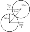 |
Fig. 1 Impact geometry and definition of the impact velocity vimp and angle θimp. |
3.2 Analysis of results
We conductsimulations of impacts and subsequent gravitational reaccumulation over a period of 1.0 ×10⁵ s. The typical timescale of reaccumulation is estimated as tacc = 2Rt∕vesc, where vesc is the two-body escape velocity of planetesimals. The value of tacc is calculatedas
 (15)
(15)
Thus, 1.0 × 10⁵ s is about 100 times longer than the typical timescale of reaccumulation, and we also confirmed that gravitational reaccumulation is sufficiently finished after 1.0 × 10⁵ s.
After collisional simulations, we identify the largest remnants using a friends-of-friends algorithm (e.g., Huchra & Geller 1982). We find a swarm of SPH particles with spacing less than 1.5h and then the largest swarm is identified with the largest remnant.
Then we evaluate the shapes of the largest remnants. To do so, we quantitatively measure the axis lengths of the largest remnants using the inertia moment tensor. We approximate the largest remnant as an ellipsoid that has the same inertia moment tensor and mass, and then we identify the axis lengths of the ellipsoid with those of the largest remnant. The detailed procedure used to calculate axis lengths is given in Appendix B. It should be noted that the bodies resulting from simulations are not perfect ellipsoids. The obtained axis ratios are thus different from those measured in the top-down method that is usually used in laboratory experiments. Therefore, the axis ratios include measurement errors of ~ 0.1 (see Michikami et al. 2018).
The shapes of objects are characterized by ratios of the lengths of the major axis a, intermediate axis b, and minor axis c, i.e., b∕a and c∕a (b∕a and c∕a are 0− 1 and b∕a > c∕a by definition). Bodies with c∕a~1 have almost spherical shapes. Bodies with b∕a ~ 1 and c∕a ≪ 1 have flat shapes. Bodies with b∕a ≪ 1 have elongated shapes.
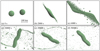 |
Fig. 2 Snapshots of the impact simulation with the impact angle θimp of 15°, the impact velocity vimp of 200 ms−1, and the totalnumber of SPH particles Ntotal of 1 × 10⁵ at 0.0 s (a), 2.0 × 10³ s (b), 6.0 × 10³ s (c), 2.0 × 10⁴ s (d), 3.0 × 10⁴ s (e), and 5.0 × 10⁴ s (f). The scale inpanel a is also valid for panels b–f. |
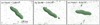 |
Fig. 3 Shapes of the largest remnants at 5.0 × 10⁴ s for the impact simulations with vimp = 200 m s−1, θimp =15°, and Ntotal = 5 × 10⁴ (a), 2 × 10⁵ (b), and 8 ×10⁵ (c). |
4 Results
4.1 Resolution dependence on the resultant shape
Figure 2 represents snapshots of the SPH simulation with the impact angle θimp of 15° and the impact velocity vimp of 200 ms−1. In Fig. 2b, the collision induces shattering of planetesimals. Then two planetesimals are stretched in the direction perpendicular to the line joining the centers of the two contacting planetesimals, and fragments are ejected (Fig. 2c). The ejected materials are mainly reaccumulated from the direction of the long axis of the largest remnant (Fig. 2d). Finally, a very elongated shape with the ratio b∕a of about 0.2is formed (Fig. 2f). The accretion on the largest body is mostly done within t ~ 5.0 × 10⁴ s.
Figure 3 shows shapes of the largest remnants at 5.0 × 10⁴ s with three different resolutions (the total number of SPH particles Ntotal of 5 × 10⁴ (a), 2 × 10⁵ (b), and 8 × 10⁵ (c)). Even if Ntotal becomes 10 times larger, the characteristic of elongated shape does not change. Figure 4 shows the dependence of the mass and axis ratios of the largest remnants on the number of SPH particles Ntotal. The mass of the largest remnants slightly decreases with increasing Ntotal because numerical dissipation by the artificial viscosity decreases for higher resolution. This tendency is the same as the result of Genda et al. (2015). The axis ratios slightly increase with increasing Ntotal, and the difference in b∕a between Ntotal of 5 × 10⁴ and 8 × 10⁵ is about 0.03. The difference in axis ratios less than 0.1 is unimportant for the analysis of asteroidal shapes because the difference in axis measurements also causes such minor errors as discussed above. Therefore, the number of SPH particles of 105 is sufficient to capture at least the feature of shapes.
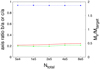 |
Fig. 4 Dependence of the mass and axis ratios of the largest remnants on the number of SPH particles Ntotal for the impact with θimp = 15° and vimp = 200 m s−1. Shown are the ratio b∕a (red solid line), the ratio c∕a (green dashed line), and the mass of the largest remnants Mlr normalized by the mass of an initial planetesimal Mtarget (blue dotted line). The left vertical axis shows the axis ratios, and right vertical axis shows the mass of the largest remnant. |
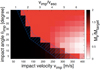 |
Fig. 5 Dependence of the mass of the largest remnants on the impact velocity vimp and the impact angle θimp. Upper horizontal axis shows vimp normalized by two-body escape velocity vesc. The mass of the largest remnants Mlr normalized by the mass of an initial planetesimal Mtarget are color-coded. Thus, Mlr∕Mtarget = 2.0 means complete merging. The hatched region approximately shows the transitional parameters from merging collisions to hit-and-run or erosive collisions. |
4.2 Mass of the largest remnants
Hereafter, we use 105 SPH particles for a simulation, and we measure the mass and axis ratios of the largest remnants at 1.0 × 10⁵ s after impacts.
Figure 5 shows the mass of the largest remnants Mlr formed through collisions with vimp = 50−400 m s−1 and θimp = 5°−45°. The increment of the velocity is 25 m s−1, and that of the angle is 5°. For θimp ≤ 15°, Mlr~ 2Mtarget due to collisional merging for low vimp, and Mlr gradually decreases with increasing vimp because of erosive collisions. The impact parameters for the transition between merging and erosive collisions are highlighted in Fig. 5. On the other hand, for θimp ≥ 20°, sharp variation in Mlr from ~2Mtarget to ~ Mtarget is seen around vimp ~ 100 m s−1. This is because collisions with high vimp result in a “hit-and-run” process where two planetesimals move apart after the collision. The transition parameters between merging and hit-and-run collisions are also highlighted in Fig. 5. The erosive nature for low θimp and merging/hit-and-run nature for high θimp are also observed in previous collisional simulations (Agnor & Asphaug 2004; Leinhardt & Stewart 2012).
For vimp > 300 m s−1, Mlr has a minimum value at θimp ≈ 15° (see Fig. 5). For head-on collisions, the most of the impact energy is dissipated and not transformed to the ejection processes, which results in large Mlr. For slightly higher θimp, the impact energy is more effectively used for ejection, and thus the mass of the largest remnant Mlr becomes smaller. However, for much higher θimp, the velocity component normal to colliding bodies is small, such that the impact energy is not effectively used for destruction and ejection, which results in larger Mlr. Therefore, an intermediate θimp yields smallest Mlr.
We note that collisions with vimp > 400 m s−1 and low θimp result in Mlr ≤ 0.1Mtarget. The largest remnants resulting from such impacts are composed of less than about 5000 SPH particles, and resolved by less than 20 SPH particles along each axis direction. Thus, axis ratios obtained from such a small number of SPH particles are not measured accurately. Our simulations of impacts with parameters outside those of Fig. 5 show that impacts with vimp = 500 m s−1 and θimp = 5−25° result in Mlr ∕Mtarget = 0.01 − 0.07. For θimp > 45°, only edges of planetesimals are destroyed by collisions rather than overall deformation, so that the investigation of such impact angles is not interesting. For example, our impact simulations with θimp = 60° and vimp = 100−500 m s−1 result in Mlr ∕Mtarget = 0.91−0.99, which means merely partial destruction. Therefore, we investigate the collisions with 50 m s−1 ≤ vimp ≤ 400 m s−1 and 5° ≤ θimp ≤ 45° because in this parameter range the resolution of the largest remnants is mainly sufficient and significant shape deformation occurs.
4.3 Characteristic shapes formed by collisions
As a result of impact simulations with 50 m s−1 ≤ vimp ≤ 400 m s−1 and 5° ≤ θimp ≤ 45°, we find thatthe resultant shapes of the largest remnants are roughly classified into five categories. In this section, we introduce the results of typical impacts to form five different characteristic shapes and catastrophic collisions.
4.3.1 Bilobed shapes
If the impact velocity is very small, the initial spherical shapes of colliding bodies are preserved and collisional merging forms bilobed shape. Figure 6 shows impact snapshots with vimp = 50 m s−1 and θimp = 30°. The impact forms a bilobed shape (Fig. 6). The two-body escape velocity vesc is about 60 ms−1, which is slightly higher than the impact velocity of this simulation. For vimp < vesc, the impact energy is too small to largely deform the initial spherical shapes (see Figs. 6b,c), and colliding bodies are gravitationally bound. Thus, the bilobed shapes resulting from such low-velocity impacts are independent of θimp.
4.3.2 Spherical shapes
The initial spherical shape is sufficiently deformed with vimp ~ 100 m s−1, which results in a single sphere due to the merging of two planetesimals. Figure 7 shows an impact producing a spherical shape with vimp = 100 m s−1 and θimp = 10°. Collisional deformation (Fig. 7b) and gravitational reaccumulation (Figs. 7c,d) results in a spherical shape.
It should be noted that a relatively low-speed collision with θimp ≥ 40° results in local destruction due to hit-and-run, whose outcome is also close to two spheres.
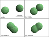 |
Fig. 6 Snapshots of the impact simulation with θimp = 30° and vimp = 50 m s−1 at 0.0 s (a), 3.5 × 10³ s (b), 1.0 × 10⁴ s (c), and 5.0 × 10⁴ s (d). |
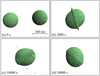 |
Fig. 7 Snapshots of the impact simulation with θimp = 10° and vimp = 100 m s−1 at 0.0 s (a), 2.0 × 10³ s (b), 1.0 × 10⁴ s (c), and 5.0 × 10⁴ s (d). |
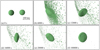 |
Fig. 8 Snapshots of the impact simulation with θimp = 5° and vimp = 200 m s−1 at 0.0 s (a), 6.0 × 10³ s (b), 1.2 × 10⁴ s (c), 1.6 × 10⁴ s (d), 2.0 × 10⁴ s (e), and 1.0 × 10⁵ s (f). |
4.3.3 Flat shapes
Figure 8 shows impact snapshots with vimp = 200 m s−1 and θimp = 5°. The initial spherical shapes are completely deformed (Figs. 8b,c), and the resultant shape is flat (Figs. 8d–f). The flat bodies are close to oblate shapes. The minor axis is formed in the direction perpendicular to the angular momentum vector.
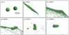 |
Fig. 9 Snapshots of the impact simulation with θimp = 20° and vimp = 250 m s−1 at 0.0 s (a), 2.0 × 10³ s (b), 1.0 × 10⁴ s (c), 2.0 × 10⁴ s (d), 5.0 × 10⁴ s (e), and 1.0 × 10⁵ s (f). |
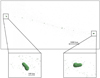 |
Fig. 10 Zoomed-out view of the impact simulation with vimp = 250 m s−1 and θimp = 20° at 1.0 × 10⁵ s. The two enlarged figures show the shape of the largest and second-largest remnants. |
4.3.4 Elongated shapes
A collision forming an extremely elongated shape is shown in Fig. 2. The collision results in Mlr~ 2Mtarget; collisional merging mainly occurs.
Some hit-and-run collisions also produce elongated shapes. Figure 9 shows snapshots of the impact with vimp = 250 m s−1 and θimp = 20°, and Fig. 10 shows a zoomed-out view of Fig. 9f. The impact results in significant destruction and deformation (Figs. 9b,c). Although two planetesimals do not merge (Fig. 10), the reaccretion of the surrounding fragments produces two elongated shapes (Figs. 9d–f and 10). We note that the largest and second-largest objects in hit-and-run collisions have almost the same shape (Fig. 10).
4.3.5 Hemispherical shapes
In Fig. 11, we show an impact forming hemispherical shapes. Significant destruction occurs around the impact point and a large number of fragments are ejected straightforwardly (Fig. 11b). This collisional truncation results in hemispherical shapes (Figs. 11c–e).
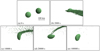 |
Fig. 11 Snapshots of the impact simulation with θimp = 45° and vimp = 350 m s−1 at 0.0 s (a), 2.0 × 10³ s (b), 1.0 × 10⁴ s (c), 2.0 × 10⁴ s (d), and 1.0 × 10⁵ s (e). |
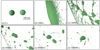 |
Fig. 12 Snapshots of the impact simulation with vimp = 400 m s−1 and θimp = 5° at 0.0 s (a), 2.0 × 10³ s (b), 2.6 × 10⁴ s (c), 5.0 × 10⁴ s (d), 8.0 × 10⁴ s (e), and 1.0 × 10⁵ s (f). |
4.3.6 Super-catastrophic destruction
Figure 12 shows the result of the impact simulation with vimp = 400 m s−1 and θimp = 5°. The impact of very high vimp produces a large curtain of ejected fragments (Fig. 12b), and the gravitational fragmentation of the curtain forms many clumps (Fig. 12c). Then the largest remnant is formed through the coalescence of clumps (Figs. 12d–f).
In collisions with Mlr < 0.4Mtarget, the largest bodies are formed through significant reaccretion of ejecta. Even a small difference in the initial conditions produces significant difference in the distribution of ejecta, which leads to a variety of shapes. Therefore, high-resolution simulations are required. We will conduct simulations with much higher number of SPH particles in a future work. In this paper, we just call impacts with Mlr < 0.4Mtarget super-catastrophic destruction, and do not classify shapes for such destructive impacts.
4.4 Summary of shapes formed by collisions
Figure 13 shows the axis ratios of the largest remnants formed by impacts with various impact velocities and angles. For hit-and-run collisions, the largest and second-largest bodies have similar shapes, as shown in Fig. 10. Thus, if the mass ratio of the largest and second-largest bodies is smaller than 2.0, we use the averaged values between two bodies for b∕a and c∕a. We note that the sharp variation in axis ratios at the hatched regions in Fig. 13 is caused by the transition between merging and erosive or hit-and-run collisions.
We categorize shapes of collisional outcomes into bilobed, spherical, flat, elongated, hemispherical, and super-catastrophic destruction as shown in Table 1. The classification given by Table 1 mainly corresponds to the shapes formed via the processes shown in Sect. 4.3. Figure 14 shows impact parameters producing the classified shapes, which indicates vimp ~ 50 m s−1, or vimp ~ 100 m s−1 and θimp > 25° (bilobed shapes), vimp ~ 100 m s−1 and θimp < 25° (spherical shapes), vimp > 100 m s−1 and vimp sinθimp < 30 m s−1 (flat shapes), vimp > 100 m s−1, vimp sinθimp > 30 m s−1, and θimp < 30° (elongated shapes), andvimp > 100 m s−1 and θimp > 30° (hemispherical shapes).
We note that two impacts resulting in flat shapes are in the elongated-shape region (vimp = 175 m s−1, θimp = 20° and vimp = 300 m s−1, θimp = 10°). These impacts correspond to elongated-shape-forming collisions with the second collision as shown in Appendix C. We consider these impacts as elongated-shape-forming collisions from the shapes observed in the simulations.
Based on the classification in Fig 14, we find the specific conditions to determine the shapes, which are written as
-
bilobed and spherical shapes: vimp < 1.6vesc,
-
flat shapes: vimp > 1.6vesc and vimp sinθimp < 0.5vesc,
-
hemispherical shapes: vimp > 1.6vesc and θimp > 30°,
and
-
elongated shapes: vimp > 1.6vesc, θimp < 30°, vimp sinθimp > 0.5vesc, and Mlr > 0.4Mtarget,
where the two-body escape velocity vesc ≈ 60 m s−1. The hatched region in Fig. 14 divides the elongated-shape region into two parts. Elongated shapes formed with parameters in the left part of the hatched region are formed by merging collisions (see Fig. 2), and those in the right part are formed by hit-and-run collisions (see Fig. 9).
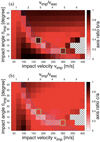 |
Fig. 13 Dependence of the ratios b∕a and c∕a of the largestremnants on vimp and θimp. The ratios b∕a (panel a) and c∕a (panel b) are color-coded according to the scale on the right. For impacts in the cross-hatched region, we do not measure the axis ratios of the largest remnants because their mass is too small (less than 0.15 Mtarget). The meaning of the hatched regions is the same as in Fig. 5. Parameters surrounded by green boxes represent impacts with the second collision as shown in Appendix C. |
Thresholds of b∕a, c∕a, and Mlr ∕Mtarget of the largestremnants for the categorization of shapes.
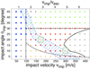 |
Fig. 14 Summary of classification of resultant shapes. Blue squares represent the impact parameters vimp and θimp producing bilobed shapes; gray triangles for spherical shapes; orange inverted triangles for flatshapes; red circles for elongated shapes; light green diamonds for hemispherical shapes; and black crosses for super-catastrophic destruction. Dotted line shows vimp =1.6vesc = 100 m s−1, dashed line shows θimp = 30°, chain curve shows vimp sinθimp = 0.5vesc = 30 m s−1, and solid curve shows Mlr = 0.4Mtarget. The meanings of the hatched region and green boxes are the same as in Fig. 13. |
5 Discussion
5.1 Four conditions required for the formation of elongated shapes
The threshold of vimp > 1.6vesc is required for significant deformation. We estimate necessary impact velocity to deform planetesimals as follows. The frictional force of μd p acts on the area of  and the energy dissipation occurs due to frictional deformation on the length scale of ~ 4Rt. The dissipated energy Edis is estimated as
 (16)
(16)
The timescale for deformation of whole bodies is estimated to be 2Rt ∕vimp, which is much longer than the shock passing time ~2Rt∕Cs, where Cs ≈ 3 km s−1 is the sound speed. High-pressure states caused by shocks are already relaxed before the end of the deformation, and shocks do not contribute to the pressure for frictional force given in Eq. (16). Therefore, the pressure is mainly determined by the self-gravity and estimated to be central pressure of a planetesimal with the radius of Rt and uniform density of ρ0, given by
 (17)
(17)
Equating the total initial kinetic energy for two equal-mass bodies  to Edis, we obtain the critical deformation velocity:
 (18)
(18)
The impactvelocity obtained in Eq. (18) closely agrees with vimp = 1.6vesc in spite of the rough estimation of the dissipated energy Edis.
The condition of θimp < 30° is needed for the avoidance of hemispherical shapes caused by hit-and-run collisions. For θimp ≥ 30° half or smaller of a target is directly interacted by an impactor, resulting in hit-and-run collisions (Asphaug 2010; Leinhardt & Stewart 2012). To form elongated shapes, it is necessary for almost the whole volume of two planetesimals to be deformed. For θimp < 30° most of the planetesimals are directly affected by collisions, which leads to deformation in the form of elongated shapes.
Collisional elongation requires high shear velocity vimp sinθimp > 0.5vesc, while impacts with vimp sinθimp < 0.5vesc produce flatshapes. Elongated shapes are formed through stretching the planetesimals in the direction of the shear velocity (seeFigs. 2, 9). However, the self-gravity prevents deformation, which occurs if vimp sinθimp ≪ vesc. We find that elongation needs vimp sinθimp > vesc∕2.
Super-catastrophic destruction with Mlr < 0.4Mtarget produces many small remnants that mainly have spherical shapes, as shown in Fig. 12. Elongated shapes may not be formed through super-catastrophic destruction. Thus, elongated shapes are mainly formed through impacts with Mlr> 0.4Mtarget.
Distribution of pressure is determined by the self-gravity unless the impact velocity is comparable to or larger than the sound speed. Since the frictional force is proportional to the pressure, the friction is also determined by the self-gravity. Thus, unless the material strength is dominant, the force on bodies (right-hand side of Eq. (2)) is solely determined by the self-gravity, so that results of impacts are characterized by dimensionless velocity vimp∕vesc regardless of the scale or size of planetesimals. For rocky planetesimals with Rt ≥ 0.5 km, the friction is dominant rather than the material strength. For Rt ≤ 200 km, vesc is less than 0.1Cs. Therefore, the conditions to form elongated shapes and the shape classification in Fig. 14 (upper horizontal axis) are also valid for equal-mass impacts with the angle of friction of 40° and 100 km≲Rt≲102 km.
5.2 Applications
We analyzed the shapes of 139 asteroids with diameters D > 80 km, obtained from the DAMIT database2. We derived the axis ratios of the asteroids in DAMIT according to the experimental method (Fujiwara et al. 1978). We found 20 irregularly shaped asteroids that have c∕a < 0.6 and D > 80 km. These irregular asteroids include elongated ones with b∕a < 0.6 ((63) Ausonia, (216) Kleopatra, (624) Hektor) and flat ones with b∕a > 0.9 and c∕a < 0.5 ((419) Aurelia, (471) Papagena). Therefore, ~10% of asteroids with D > 80 km have irregular shapes. We note that this fraction may become smaller because DAMIT preferentially contains irregularly shaped asteroids due to the light-curve inversion technique. However, in spite of the error, DAMIT seems to accurately measure b∕a for asteroids with b∕a < 0.6. For example, b∕a of asteroid Itokawa obtained from the light curve is 0.5 (Kaasalainen et al. 2003), which is a similar value to b∕a = 0.55 obtained from the in situ observation (Fujiwara et al. 2006). Therefore, we discuss the statistics of asteroidal shapes based on DAMIT.
(624) Hektor is a Jupiter trojan, and the others are main-belt asteroids. In the main belt, the Keplerian velocity is vK ≈ 20 km s^-1 and the mean impact velocity is roughly estimated to be  with the mean orbital eccentricity of eave = 0.15 and inclination of iave = 0.13 (Ueda et al. 2017). This mean impact velocity is much higher than that treated in our simulations (vimp < 400 m s−1). We estimate the distribution of impact velocities between main-belt asteroids using the orbital parameters obtained from the JPL small-body Database Search Engine3 and the method for obtaining the relative velocity at the orbital crossing according to Kobayashi & Ida (2001). This gives the mean collisional velocity of 5 kms−1. The probability that impact velocities become less than 400 m s−1 is about 0.15%. Therefore, the expected production of irregularly shaped asteroids due to low-velocity impacts in the present solar system is too low to reproduce their current fraction.
Similar-mass impacts with the mean impact velocity in the main belt result in catastrophic destruction, which also produces irregular shapes and asteroid families. An irregularly shaped asteroid formed through a recent catastrophic destruction may be contained in an asteroid family. According to the AstDyS-2 database4, among 20 irregularly shaped asteroids with D > 80 km that we find in DAMIT, only three ((20) Massalia, (63) Ausonia, (624) Hektor) are contained in asteroid families. However, (20) Massalia and (624) Hektor are the largest remnants of asteroid families that are formed through cratering impacts (Vokrouhlický et al. 2006; Rozehnal et al. 2016). Thus, 19 out of these 20 irregularly shaped asteroids were probably not formed through recent catastrophic destruction. Catastrophic destruction is the minor process for the formation of irregular shapes of large asteroids, which is consistent with their collisional lifetimes estimated to be much longer than the age of the solar system (O’Brien & Greenberg 2005).
Bilobed shapes are also formed through largely destructive impacts. Many remnants are formed in a large curtain of ejected fragments (see Fig. 12) and then these remnants may again collide with each other with vimp~vesc, which leads to the formation of bilobed shapes. We additionally conduct a higher resolution simulation of a largely destructive impact, which shows that bilobed asteroids are formed. However, flat shapes are not formed in the destructive impact.
For impacts with high mass ratios, deformation occurs on the scale of impactors, which is much smaller than that of targets, so that overall deformation does not occur via a single collision. Our additional simulations with impactor-to-target mass ratio 1/64 show that non-disruptive impacts (Mlr > 0.5Mtarget) with various impact velocities of vimp = 500–3000 m s−1 and angles of θimp = 0–40° do not form irregular shapes with c∕a≲0.7. Although such impacts are frequent, isotropic impacts to almost spherical asteroids do not form irregular shapes.
Therefore, irregular shapes of asterodes with D > 80 km, especially flat shapes, are likely to be formed through similar-mass and low-velocity impacts, which are unlikely to occur in the present solar system. Relative velocities between planetesimals are increased by gravitational interaction with planets, especially Jupiter (e.g., Kobayashi et al. 2010). Thus, collisional velocities in the main belt may be much lower prior to Jupiter formation. Jupiter formation may significantly deplete asteroids (Bottke et al. 2005), and similar-mass impacts may be frequent prior to Jupiter formation. Irregularly shaped asteroids are possibly formed in such environments. Therefore, irregularly shaped asteroids with D > 80 km may be formed in the primordial environment and remain the same until today.
6 Summary
Asteroids are believed to be remnants of planetesimals formed in the planet formation era and may retain information of the history of the solar system. Irregular shapes of asteroids can be formed through collisional destruction and coalescence of planetesimals. Thus, clarifying the impact conditions needed to form specific shapes of asteroids can constrain the epoch or collisional environment forming those asteroids.
Our simulations show the relationship between the impact conditions and the resultant shapes of planetesimals. We carried out simulations of collisions between planetesimals using the SPH method for elastic dynamics with self-gravity and the models for fracture and friction. We considered collisions between two planetesimals with radius of 50 km because significant shape deformation occurs in equal-mass impacts. We varied the impact velocity vimp from 50 to 400 m s−1 and the impact angle θimp from 5° to 45°. Then we measured the shape of the largest remnant formed in each impact simulation.
We confirm that various shapes are formed by equal-mass impacts. We classify the shapes of the largest remnants into five categories if the mass of the largest remnant Mlr is larger than 0.4 of that of an initial planetesimal Mtarget. The result of the shape classification is as follows:
-
For vimp ~ 50 m s−1, or vimp ~ 100 m s−1 and θimp > 25°, bilobed shapes are formed because the planetesimals merge and preserve the initial spherical shapes (see Fig. 6).
-
For vimp ~ 100 m s−1 and θimp < 20°, spherical shapes are formed because a part of the planetesimal is crushed (see Fig. 7).
-
For vimp > 100 m s−1 and vimp sinθimp < 30 m s−1, flat shapes are formed because of nearly head-on collisions and larger deformation (see Fig. 8).
-
For vimp > 100 m s−1, vimp sinθimp > 30 m s−1, and θimp < 30°, elongated shapes are formed because planetesimals are stretched in the direction perpendicular to the line joining the centers of the two contacting planetesimals (see Fig. 2).
-
For vimp > 100 m s−1 and θimp > 30°, hemispherical shapes are formed because of the excavation of the edges of the planetesimals (see Fig. 11).
As a result of the shape classification, we find four conditions to form elongated shapes with the ratio b∕a lower than 0.7. The four conditions and their meanings are as follows:
-
vimp > 1.6vesc: overall deformation of the planetesimals requires large impact velocity.
-
θimp < 30°: impacts with large impact angles result in the erosion of only the edges of the planetesimals.
-
vimp sinθimp > 0.5vesc: elongated shapes are formed through the stretching of the planetesimals in the direction of the shear velocity vimp sinθimp, so that high shear velocity is also required.
-
Mlr > 0.4Mtarget: in largely destructive impacts the largest remnants are formed through violent reaccumulation of fragments and the resultant shapes tend to be spherical.
As we discussed in Sect. 5.1, these conditions are also valid for equal-mass impacts with the angle of friction of 40° and 100 km≲Rt≲102 km, although wehave not yet confirmed this through numerical experiments.
According to our simulations, various irregular shapes are formed through impacts with two equal-mass planetesimals and low impact velocities < 400 m s−1. Impacts with an average relative velocity in the main belt ≈5 km s−1 mainly result in catastrophic destruction for similar-mass impacts or moderate destruction for impacts with high mass ratios. However, both catastrophic destruction and impacts with high mass ratios are unlikely to produce flat shapes, as we discussed in Sect 5.2, based on our additional simulations. Asteroids with diameters > 80 km have longer collisional lifetimes than the age of the solar system. Therefore, we suggest that irregular shapes of asteroids with diameters > 80 km, especially flat shapes, are likely to be formed through similar-mass and low-velocity impacts in the primordial environment prior to the formation of Jupiter.
We only consider collisions between two rocky planetesimals with radius of 50 km and the limited impact velocity range. Thus, investigations of the following impacts are for our future work: impacts with different radii of planetesimals, high mass ratios of two colliding planetesimals, and higher impact velocities that form smaller fragments. Clarifying more detailed relationships between impact conditions and the resultant shapes of planetesimals may allow us to extract more detailed information on the history of the solar system from the shapes of asteroids.
Acknowledgements
[Acknowledgement] We thank Hidekazu Tanaka and Ryuki Hyodo for the useful discussions and comments, and Martin Jutzi and Natsuki Hosono for giving us the useful information about the numerical simulation methods. We also thank the anonymous reviewer for the valuable and detailed comments on our manuscript. K.S. is supported by JSPS KAKENHI grant No. JP 17J01703. H.K. and S.I. are supported by Grant-in-Aid for Scientific Research (18H05436, 18H05437, 18H05438, 17K05632, 17H01105, 17H01103, 23244027, 16H02160). Numerical simulations in this work were carried out on Cray XC30 at the Center for Computational Astrophysics, National Astronomical Observatory of Japan.
Appendix A Time development method
Here, we describe the detailed equation of the leapfrog integrator used in this study. At the nth step, we update the position of the ith particle  and other quantities ofthe ith particle
  as
as
![\begin{align*} &\bm{x}_{i}^{n+1}=\bm{x}_{i}^{n}+\bm{v}_{i}^{n}\Delta t + \frac{1}{2}\left(\frac{\textrm{d}\bm{v}_{i}}{\textrm{d}t}\right)^{n}\Delta t^{2},\nonumber \\ &q_{i}^{n+1}=q_{i}^{n}+\frac{1}{2}\left[\left(\frac{\textrm{d}q_{i}}{\textrm{d}t} \right)^{n} + \left(\frac{\textrm{d}q_{i}}{\textrm{d}t} \right)^{n+1} \right]\Delta t, \tag{A.1}\end{align*}](/articles/aa/full_html/2018/12/aa33227-18/aa33227-18-eq31.png) (A.1)
(A.1)
where Δt is the time step.
In Eq. (A.1), for example,  is determined by
  . However, to calculate
  with the equation of motion (2), we need
  , so that we cannot directly derive
  . Thus, we update the physical quantities with the following procedure. First, we predict the quantities of the (n + 1)th step, only using the quantities of the nth step as
 (A.2)
(A.2)
At the same time, we update the positions as Eq. (A.1). Then we calculate  using
using  and
and  , and we obtain
  from Eq. (A.1). We can reuse
  at the next step, so we calculate derivatives of variables only once at every step. Moreover, if all variables vary linearly in time, this procedure does not produce any integration error. Therefore, this integration scheme has second-order accuracy in time.
The time step Δt is determined by considering the Courant condition as
 (A.3)
(A.3)
where Cs,i is local bulk sound speed at the position of the ith particle. The value of Cs,i is calculated from the equation of state, the density, the specific internal energy, and the pressure of the ith particle. We adopt the value of CCFL = 0.5.
Appendix B Measurement of axis lengths of the largest remnants
The inertia moment tensor of the largest remnant composed of k SPH particles is calculated as
![\begin{equation*} I^{\alpha \beta}=\sum_{k}m_{k}\left[(x_{k}^{\gamma}-x_{\textrm{CoM}}^{\gamma})(x_{k}^{\gamma}-x_{\textrm{CoM}}^{\gamma})\delta^{\alpha \beta} - (x_{k}^{\alpha}-x_{\textrm{CoM}}^{\alpha})(x_{k}^{\beta}-x_{\textrm{CoM}}^{\beta}) \right],\end{equation*}](/articles/aa/full_html/2018/12/aa33227-18/aa33227-18-eq44.png) (B.1)
(B.1)
where xCoM is the position vector at the center of mass of the largest remnant. Then, three principal moments of inertia I1, I2, and I3 are obtained
from Iαβ. Here, I1 > I2 > I3. For a uniform ellipsoid with the length of major axis a, intermediate axis b, and minor axis c, the three principal moments of inertia are represented as
 (B.2)
(B.2)
Equation (B.2) is rewritten as
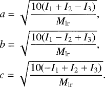 (B.3)
(B.3)
Therefore, we obtain I1, I2, I3, and Mlr of the largest remnant through a simulation, and then derive its a, b, and c from Eq. (B.3).
Appendix C Elongated shape-forming impacts with the second collisions
Figure C.1 represents a collision with vimp = 175 m s−1 and θimp = 20°, which results in the second collision of two elongated objects. As in Fig. 2, the first collision produces two elongated objects (Figs. C.1b,c). However, the energy dissipation by the collision makes colliding bodies gravitationally bounded (Fig. C.1d), and the resultant body formed by the merging is no longer an elongated object (Fig. C.1e). Although the resultant body is not elongated, this impact should also be classified as an elongated shape-forming collision.
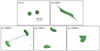 |
Fig. C.1 Snapshots of the impact simulation with vimp = 175 m s−1 and θimp = 20° at 0.0 s (panel a), 4.0 × 10³ s (panel b), 3.0 × 10⁴ s (panel c), 7.0 × 10⁴ s (panel d), and 1.0 × 10⁵ s (panel e). |
References
- Agnor, C., & Asphaug, E. 2004, ApJ, 613, 157 [Google Scholar]
- Asphaug, E. 2010, Chem. Erde/Geochem., 70, 199 [Google Scholar]
- Benz, W., & Asphaug, E. 1995, Comput. Phys. Commun., 87, 253 [NASA ADS] [CrossRef] [Google Scholar]
- Benz, W., & Asphaug, E. 1999, Icarus, 142, 5 [NASA ADS] [CrossRef] [Google Scholar]
- Bonet, J., & Lok, T.-S. L. 1999, Comput. Methods Appl. Mech. Eng., 180, 97 [NASA ADS] [CrossRef] [Google Scholar]
- Bottke, W. F. Jr., Durda, D. D., Nesvorný, D., et al. 2005, Icarus, 175, 111 [NASA ADS] [CrossRef] [Google Scholar]
- Cibulková, H., Ďurech, J., Vokrouhlický, D., & Oszkiewicz, D. A. 2016, A&A, 596, A57 [NASA ADS] [CrossRef] [EDP Sciences] [Google Scholar]
- Ďurech, J., Sidorin, V., & Kaasalainen, M. 2010, A&A, 513, A46 [NASA ADS] [CrossRef] [EDP Sciences] [Google Scholar]
- Fujiwara, A., Kamimoto, G., & Tsukamoto, A. 1978, Nature, 272, 602 [NASA ADS] [CrossRef] [Google Scholar]
- Fujiwara, A., Kawaguchi, J., Yeomans, D. K., et al. 2006, Science, 312, 1330 [NASA ADS] [CrossRef] [PubMed] [Google Scholar]
- Genda, H., Kokubo, E., & Ida, S. 2012, ApJ, 744, 137 [NASA ADS] [CrossRef] [Google Scholar]
- Genda, H., Fujita, T., Kobayashi, H., Tanaka, H., & Abe, Y. 2015, Icarus, 262, 58 [NASA ADS] [CrossRef] [Google Scholar]
- Grady, D. E., & Kipp, M. E. 1980, Int. J. Rock Mech. Min. Sci. Geomech. Abstr., 17, 147 [Google Scholar]
- Greenberg, R., Wachker, J. F., Hartmann, W. K., & Chapman, C. R. 1978, Icarus, 35, 1 [NASA ADS] [CrossRef] [Google Scholar]
- Hayashi, C., Nakazawa, K., & Nakagawa, Y. 1985, in Protostars and Planets II, eds. D. C. Black & M. S. Matthews, 1100 [Google Scholar]
- Heiken, G. H., Vaniman, D. T., & French, B. M. 1991, Lunar Sourcebook – A User’s Guide to the Moon [Google Scholar]
- Hubber, D. A., Allison, R. J., Smith, R., & Goodwin, S. P. 2013, MNRAS, 430, 1599 [NASA ADS] [CrossRef] [Google Scholar]
- Huchra, J. P.,& Geller, M. J. 1982, ApJ, 257, 423 [NASA ADS] [CrossRef] [Google Scholar]
- Inaba, S., Wetherill, G. W., & Ikoma, M. 2003, Icarus, 166, 46 [NASA ADS] [CrossRef] [Google Scholar]
- Inutsuka, S. 2002, J. Comput. Phys., 179, 238 [NASA ADS] [CrossRef] [Google Scholar]
- Iwasawa, M., Tanikawa, A., Hosono, N., et al. 2015, in Proceedings of the 5th International Workshop on Domain-Specific Languages and High-Level Frameworks for High Performance Computing, WOLFHPC ’15 (New York, NY: ACM), 1:1 [Google Scholar]
- Iwasawa, M., Tanikawa, A., Hosono, N., et al. 2016, PASJ, 68, 541 [Google Scholar]
- Jutzi, M. 2015, Planet. Space Sci., 107, 3 [NASA ADS] [CrossRef] [Google Scholar]
- Jutzi, M., & Asphaug, E. 2015, Science, 348, 1355 [NASA ADS] [CrossRef] [Google Scholar]
- Jutzi, M., & Benz, W. 2017, A&A, 597, A62 [NASA ADS] [CrossRef] [EDP Sciences] [Google Scholar]
- Kaasalainen, M., Kwiatkowski, T., Abe, M., et al. 2003, A&A, 405, L29 [NASA ADS] [CrossRef] [EDP Sciences] [Google Scholar]
- Kobayashi, H., & Ida, S. 2001, Icarus, 153, 416 [NASA ADS] [CrossRef] [Google Scholar]
- Kobayashi, H., & Tanaka, H. 2018, ApJ, 862, 127 [NASA ADS] [CrossRef] [Google Scholar]
- Kobayashi, H., Tanaka, H., Krivov, A. V., & Inaba, S. 2010, Icarus, 209, 836 [NASA ADS] [CrossRef] [Google Scholar]
- Kobayashi, H., Tanaka, H., & Okuzumi, S. 2016, ApJ, 817, 105 [NASA ADS] [CrossRef] [Google Scholar]
- Kokubo, E., & Ida, S. 1996, Icarus, 123, 180 [NASA ADS] [CrossRef] [Google Scholar]
- Kokubo, E., & Ida, S. 1998, Icarus, 131, 171 [NASA ADS] [CrossRef] [Google Scholar]
- Leinhardt, Z. M., & Stewart, S. T. 2012, ApJ, 745, 79 [NASA ADS] [CrossRef] [Google Scholar]
- Libersky, L. D., & Petschek, A. G. 1991, in Advances in the Free-Lagrange Method Including Contributions on Adaptive Gridding and the Smooth Particle Hydrodynamics Method, eds. H. E. Trease, M. F. Fritts, & W. P. Crowley (Berlin: Springer) Lect. Notes Phys., 395, 248 [NASA ADS] [CrossRef] [Google Scholar]
- Marchis, F., Ďurech, J., Castillo-Rogez, J., et al. 2014, ApJ, 783, L37 [NASA ADS] [CrossRef] [Google Scholar]
- Michel, P., & Richardson, D. C. 2013, A&A, 554, L1 [NASA ADS] [CrossRef] [EDP Sciences] [Google Scholar]
- Michikami, T., Kadokawa, T., Tsuchiyama, A., et al. 2018, Icarus, 302, 109 [NASA ADS] [CrossRef] [Google Scholar]
- Monaghan, J. J. 1992, ARA&A, 30, 543 [NASA ADS] [CrossRef] [Google Scholar]
- O’Brien, D. P., & Greenberg, R. 2005, Icarus, 178, 179 [NASA ADS] [CrossRef] [Google Scholar]
- Petit, J.-M., Morbidelli, A., & Chambers, J. 2001, Icarus, 153, 338 [NASA ADS] [CrossRef] [Google Scholar]
- Rozehnal, J., Brož, M., Nesvorný, D., et al. 2016, MNRAS, 462, 2319 [NASA ADS] [CrossRef] [Google Scholar]
- Safronov, V. S. 1969, Evolution of the protoplanetary cloud and formation of the Earth and the planets (Moscow: Nauka) [Google Scholar]
- Schwartz, S. R., Michel, P., Jutzi, M., et al. 2018, Nat. Astron., 2, 379 [NASA ADS] [CrossRef] [Google Scholar]
- Storrs, A., Weiss, B., Zellner, B., et al. 1999, Icarus, 137, 260 [NASA ADS] [CrossRef] [Google Scholar]
- Sugiura, K., & Inutsuka, S. 2016, J. Comput. Phys., 308, 171 [NASA ADS] [CrossRef] [Google Scholar]
- Sugiura, K., & Inutsuka, S. 2017, J. Comput. Phys., 333, 78 [NASA ADS] [CrossRef] [Google Scholar]
- Tillotson, J. H. 1962, General Atomic Report, GA-3216, 1 [Google Scholar]
- Ueda, T., Kobayashi, H., Takeuchi, T., et al. 2017, AJ, 153, 232 [NASA ADS] [CrossRef] [Google Scholar]
- Vokrouhlický, D., Brož, M., Bottke, W. F., Nesvorný, D., & Morbidelli, A. 2006, Icarus, 182, 118 [NASA ADS] [CrossRef] [Google Scholar]
- Walsh, K. J., Morbidelli, A., Raymond, S. N., O’Brien, D. P., & Mandell, A. M. 2011, Nature, 475, 206 [NASA ADS] [CrossRef] [PubMed] [Google Scholar]
- Wetherill, G. W., & Stewart, G. R. 1989, Icarus, 77, 330 [NASA ADS] [CrossRef] [Google Scholar]
- Wetherill, G. W., & Stewart, G. R. 1993, Icarus, 106, 190 [NASA ADS] [CrossRef] [PubMed] [Google Scholar]
These SPH equations are based on those of Libersky & Petschek (1991). In Sugiura & Inutsuka (2016, 2017), we extended the Godunov SPH method (Inutsuka 2002) to elastic dynamics, which can suppress the tensile instability (numerical instability that is prominent in the tension dominated region) and treat strong shock waves accurately. However, the tensile instability is insignificant because of rock fracturing, and we do not treat strong shock waves because of small impact velocities compared to sound speed. Our Godunov SPH method has excellent capabilities; however, it has a high computational cost. Thus, to conduct many simulations with various parameters, we utilize a standard SPH method in this paper.
All Tables
Thresholds of b∕a, c∕a, and Mlr ∕Mtarget of the largestremnants for the categorization of shapes.
All Figures
|
Fig. 1 Impact geometry and definition of the impact velocity vimp and angle θimp. |
| In the text | |
|
Fig. 2 Snapshots of the impact simulation with the impact angle θimp of 15°, the impact velocity vimp of 200 ms−1, and the totalnumber of SPH particles Ntotal of 1 × 10⁵ at 0.0 s (a), 2.0 × 10³ s (b), 6.0 × 10³ s (c), 2.0 × 10⁴ s (d), 3.0 × 10⁴ s (e), and 5.0 × 10⁴ s (f). The scale inpanel a is also valid for panels b–f. |
| In the text | |
|
Fig. 3 Shapes of the largest remnants at 5.0 × 10⁴ s for the impact simulations with vimp = 200 m s−1, θimp =15°, and Ntotal = 5 × 10⁴ (a), 2 × 10⁵ (b), and 8 ×10⁵ (c). |
| In the text | |
|
Fig. 4 Dependence of the mass and axis ratios of the largest remnants on the number of SPH particles Ntotal for the impact with θimp = 15° and vimp = 200 m s−1. Shown are the ratio b∕a (red solid line), the ratio c∕a (green dashed line), and the mass of the largest remnants Mlr normalized by the mass of an initial planetesimal Mtarget (blue dotted line). The left vertical axis shows the axis ratios, and right vertical axis shows the mass of the largest remnant. |
| In the text | |
|
Fig. 5 Dependence of the mass of the largest remnants on the impact velocity vimp and the impact angle θimp. Upper horizontal axis shows vimp normalized by two-body escape velocity vesc. The mass of the largest remnants Mlr normalized by the mass of an initial planetesimal Mtarget are color-coded. Thus, Mlr∕Mtarget = 2.0 means complete merging. The hatched region approximately shows the transitional parameters from merging collisions to hit-and-run or erosive collisions. |
| In the text | |
|
Fig. 6 Snapshots of the impact simulation with θimp = 30° and vimp = 50 m s−1 at 0.0 s (a), 3.5 × 10³ s (b), 1.0 × 10⁴ s (c), and 5.0 × 10⁴ s (d). |
| In the text | |
|
Fig. 7 Snapshots of the impact simulation with θimp = 10° and vimp = 100 m s−1 at 0.0 s (a), 2.0 × 10³ s (b), 1.0 × 10⁴ s (c), and 5.0 × 10⁴ s (d). |
| In the text | |
|
Fig. 8 Snapshots of the impact simulation with θimp = 5° and vimp = 200 m s−1 at 0.0 s (a), 6.0 × 10³ s (b), 1.2 × 10⁴ s (c), 1.6 × 10⁴ s (d), 2.0 × 10⁴ s (e), and 1.0 × 10⁵ s (f). |
| In the text | |
|
Fig. 9 Snapshots of the impact simulation with θimp = 20° and vimp = 250 m s−1 at 0.0 s (a), 2.0 × 10³ s (b), 1.0 × 10⁴ s (c), 2.0 × 10⁴ s (d), 5.0 × 10⁴ s (e), and 1.0 × 10⁵ s (f). |
| In the text | |
|
Fig. 10 Zoomed-out view of the impact simulation with vimp = 250 m s−1 and θimp = 20° at 1.0 × 10⁵ s. The two enlarged figures show the shape of the largest and second-largest remnants. |
| In the text | |
|
Fig. 11 Snapshots of the impact simulation with θimp = 45° and vimp = 350 m s−1 at 0.0 s (a), 2.0 × 10³ s (b), 1.0 × 10⁴ s (c), 2.0 × 10⁴ s (d), and 1.0 × 10⁵ s (e). |
| In the text | |
|
Fig. 12 Snapshots of the impact simulation with vimp = 400 m s−1 and θimp = 5° at 0.0 s (a), 2.0 × 10³ s (b), 2.6 × 10⁴ s (c), 5.0 × 10⁴ s (d), 8.0 × 10⁴ s (e), and 1.0 × 10⁵ s (f). |
| In the text | |
|
Fig. 13 Dependence of the ratios b∕a and c∕a of the largestremnants on vimp and θimp. The ratios b∕a (panel a) and c∕a (panel b) are color-coded according to the scale on the right. For impacts in the cross-hatched region, we do not measure the axis ratios of the largest remnants because their mass is too small (less than 0.15 Mtarget). The meaning of the hatched regions is the same as in Fig. 5. Parameters surrounded by green boxes represent impacts with the second collision as shown in Appendix C. |
| In the text | |
|
Fig. 14 Summary of classification of resultant shapes. Blue squares represent the impact parameters vimp and θimp producing bilobed shapes; gray triangles for spherical shapes; orange inverted triangles for flatshapes; red circles for elongated shapes; light green diamonds for hemispherical shapes; and black crosses for super-catastrophic destruction. Dotted line shows vimp =1.6vesc = 100 m s−1, dashed line shows θimp = 30°, chain curve shows vimp sinθimp = 0.5vesc = 30 m s−1, and solid curve shows Mlr = 0.4Mtarget. The meanings of the hatched region and green boxes are the same as in Fig. 13. |
| In the text | |
|
Fig. C.1 Snapshots of the impact simulation with vimp = 175 m s−1 and θimp = 20° at 0.0 s (panel a), 4.0 × 10³ s (panel b), 3.0 × 10⁴ s (panel c), 7.0 × 10⁴ s (panel d), and 1.0 × 10⁵ s (panel e). |
| In the text | |
Current usage metrics show cumulative count of Article Views (full-text article views including HTML views, PDF and ePub downloads, according to the available data) and Abstracts Views on Vision4Press platform.
Data correspond to usage on the plateform after 2015. The current usage metrics is available 48-96 hours after online publication and is updated daily on week days.
Initial download of the metrics may take a while.