| Issue |
A&A
Volume 685, May 2024
|
|
|---|---|---|
| Article Number | A86 | |
| Number of page(s) | 8 | |
| Section | Planets and planetary systems | |
| DOI | https://doi.org/10.1051/0004-6361/202346519 | |
| Published online | 14 May 2024 | |
Protoplanet collisions: New scaling laws from smooth particle hydrodynamics simulations
1
Department of Physics, New York University Abu Dhabi,
PO Box 129188,
Abu Dhabi,
UAE
e-mail: sc6459@nyu.edu
2
Center for Astrophysics and Space Science (CASS), New York University Abu Dhabi,
PO Box 129188,
Abu Dhabi,
UAE
3
Center for Space Science, NYUAD Research Institute, New York University Abu Dhabi,
PO Box 129188,
Abu Dhabi,
UAE
Received:
28
March
2023
Accepted:
30
January
2024
One common approach for solving collisions between protoplanets in simulations of planet formation is to employ analytical scaling laws. The most widely used one was developed by Leinhardt & Stewart (2012, ApJ, 745, 79) from a catalog of ~180 N-body simulations of rubble–pile collisions. In this work, we use a new catalogue of more than 20 000 SPH simulations to test the validity and the prediction capability of Leinhardt & Stewart (2012, ApJ, 745, 79) scaling laws. We find that these laws overestimate the fragmentation efficiency in the merging regime and they are not able to properly reproduce the collision outcomes in the super-catastrophic regime. In the merging regime, we also notice a significant dependence between the collision outcome, in terms of the largest remnant mass, and the relative mass of the colliding protoplanets. Here, we present a new set of scaling laws that are able to better predict the collision outcome in all regimes and it is also able to reproduce the observed dependence on the mass ratio. We compare our new scaling laws against a machine learning approach and obtain similar prediction efficiency.
Key words: astronomical databases: miscellaneous / celestial mechanics / minor planets, asteroids: general / planets and satellites: formation / planets and satellites: physical evolution / planets and satellites: terrestrial planets
© The Authors 2024
 Open Access article, published by EDP Sciences, under the terms of the Creative Commons Attribution License (https://creativecommons.org/licenses/by/4.0), which permits unrestricted use, distribution, and reproduction in any medium, provided the original work is properly cited.
This article is published in open access under the Subscribe to Open model. Subscribe to A&A to support open access publication.
1 Introduction
Pairwise collisions are considered to be the main mechanism that drives the growth of planetesimals (~100 km sized rocky bodies) into terrestrial planets, particularly inside the water snow line (e.g. Wetherill 1980; Kokubo & Ida 1996; Chambers 2001; Izidoro et al. 2017). Including collisions in simulations of terrestrial planet formation, however, has proven to be particularly challenging for two main reasons. First, the typical timescales involved in collisions are several orders of magnitude shorter than the orbital period of planetesimals (Benz et al. 2007; Kegerreis et al. 2020). Second, it is computationally challenging to fully resolve and integrate the evolution of all the material ejected during the collision, which ranges from gaseous material, such as the atmosphere and vaporised rock and water, to solid fragments the size of large asteroids (Leinhardt & Stewart 2012; Kegerreis et al. 2020; Crespi et al. 2021).
The first challenge can be overcome by employing symplectic and hybrid-symplectic integrators such as SyMBA (Duncan et al. 1998) and MERCURY (Chambers 1999), which are able to integrate close-encounters and collisions without significantly affecting the integration precision. The second challenges is still remains an open question. Various approaches have been tested in the recent decades. The most simple approach is to consider all the collisions to result in the inelastic merging of the two colliders. This approximation has been able to efficiently reproduce the fundamental characteristics of the Solar System, proving the importance of the role played by collisions between protoplanets in the evolution of planetary systems (Wetherill 1994; Chambers & Wetherill 1998; Quintana et al. 2002, 2016; Raymond et al. 2004, 2006; O'Brien et al. 2006). However, recent studies have shown that, when collisions are assumed to be inelastic, the formation timescale of terrestrial planets is significantly reduced, and both the mass and the water content of the final population of planets are overestimated (Chambers 2013; Leinhardt et al. 2015; Burger et al. 2018, 2020). On the other hand, the impact of fragmentation on the evolution of terrestrial planets remains a topic of debate, particularly when investigating the formation of close-in planets in the observed population (e.g. Mustill et al. 2018; Poon et al. 2020; Esteves et al. 2022).
A more sophisticated approach is to allow fragmentation during collisions and to estimate the properties of the main post-collisional bodies by resorting to scaling laws (e.g. Chambers 2013; Quintana et al. 2016, Wallace et al. 2017, Mustill et al. 2018; Clement et al. 2019a,b, 2022; Poon et al. 2020, Ishigaki et al. 2021). Utilizing direct N-body simulations of collisions between rubble–pile differentiated protoplanets (Leinhardt et al. 2000), Kokubo & Genda (2010) and Leinhardt & Stewart (2012), derived empirical formulae to estimate the mass of the main collisional remnants. In particular, the widely used scaling laws from the pioneering work of Leinhardt & Stewart (2012, hereafter LS12) allow one to directly estimate the mass of the first and second largest remnant given the collision properties. However, the dataset used to derive the LS12 scaling laws, (of around 180 simulations) was limited to a total of 23 datapoints in the mass range between 10−3−10 M⊕, of which only 3 datapoints were in the super-catastrophic regime.
Over the past few years, extensive catalogues of smooth particle hydrodynamics1 (SPH) simulations of collisions have been performed and are now available. In particular, Burger et al. (2020) conducted a series of 48 simulations to explore terrestrial planet formation, incorporating on-the-fly SPH simulations to model collisions. This effort yielded a collection of 9980 simulations of collision between protoplanets. Additionally, Winter et al. (2023) expanded their previous catalogue of 858 SPH simulations (presented in Crespi et al. 2021) by more than ten times by conducting 10 164 new simulations, which also accounted for the rotational momentum of the colliding bodies.
In this work, we make use of these new catalogues of SPH simulations to test and improve the LS12 scaling laws. We propose a new version of their model that is more accurate in predicting the mass of the largest post-collisional remnant. Furthermore, we validate this new set of scaling laws by comparing its prediction efficiency against a machine learning approach. In Sect. 2, we present (i) the new best fit parameters for LS12 scaling laws, (ii) a new set of scaling laws, and (iii) the machine learning model used to test and validate the new scaling law. The last section is devoted to the discussion of our results and the main conclusions.
Three catalogues used in this study (top) and catalogues used in LS12 for gravity-dominated bodies (bottom).
2 Improved fits to the new SPH dataset
The original dataset used by LS12 to derive their scaling law spans from kilometer-sized bodies to 10 Earth-mass bodies. Thanks to this wide range of masses, the authors were able to observe a transition between collisions involving small weak bodies and collisions between larger gravity-dominated bodies, with a transition point around ~10−2 M⊕. While the scaling laws are the same in the two regimes, the parameters that govern the scaling law differ. Here, we decided to focus on collision between gravity-dominated bodies only, since the new dataset of SPH simulations used in this study mainly involve gravity–dominated bodies. We refer the reader to the works of Burger et al. (2020), Crespi et al. (2021) and Winter et al. (2023) for more details on the three catalogues of SPH simulations. A summary of these catalogues, together with the datasets used by LS12, is presented in Table 1 for convenience.
2.1 Analytical fits
Based on the model adopted in LS12, the mass of the largest post–collisional remnant (Mlr), scaled by the total mass involved in the collision (Mtot), can be expressed as the function of the relative impact energy (QR) scaled by the catastrophic disruption criterion (![$\[\${\mathcal{Q}}_{\mathrm{RD}}^{*}$\]$](/articles/aa/full_html/2024/05/aa46519-23/aa46519-23-eq1.png) ). This relation can be written as:
). This relation can be written as:
![$\[\frac{M_{\mathrm{lr}}}{M_{\mathrm{tot}}}=\left\{\begin{array}{c}{{1-0.5\,\frac{Q_{\mathrm{R}}}{Q_{\mathrm{RD}}^{*}}}}\\ {{\frac{0.1}{1.8^{\eta}}\left(\frac{Q_{\mathrm{R}}}{Q_{\mathrm{RD}}^{*}}\right)^{\eta}}}\end{array}\begin{array}{c}{{\mathrm{for}\,\frac{Q_{\mathrm{R}}}{Q_{^\mathrm{RD}}^{*}}\lt 1.8}}\\ {{\mathrm{for}\,\frac{Q_{\mathrm{R}}}{Q_{\mathrm{RD}}^{*}}\gt 1.8.}}\end{array}\right.\]$](/articles/aa/full_html/2024/05/aa46519-23/aa46519-23-eq2.png) (1)
(1)
In the first branch, often referred to as universal law, LS12 assume linearity between the impact energy and the largest remnant mass, with the catastrophic disruption criterion (![$\[\${\mathcal{Q}}_{\mathrm{RD}}^{*}$\]$](/articles/aa/full_html/2024/05/aa46519-23/aa46519-23-eq3.png) ) defined as the energy at which half of the total mass is dispersed. The assumption of linearity, presented also in previous works (Stewart & Leinhardt 2009; Leinhardt et al. 2009), is a good model to use in the context of collisions with energies that are close to the catastrophic disruption criterion. However, this assumption actually fails to properly represent collisions with low-impact energy (QR/
) defined as the energy at which half of the total mass is dispersed. The assumption of linearity, presented also in previous works (Stewart & Leinhardt 2009; Leinhardt et al. 2009), is a good model to use in the context of collisions with energies that are close to the catastrophic disruption criterion. However, this assumption actually fails to properly represent collisions with low-impact energy (QR/![$\[\${\mathcal{Q}}_{\mathrm{RD}}^{*}$\]$](/articles/aa/full_html/2024/05/aa46519-23/aa46519-23-eq4.png) ≲ 0.1) as well as collisions with high impact energy (QR/
≲ 0.1) as well as collisions with high impact energy (QR/![$\[\${\mathcal{Q}}_{\mathrm{RD}}^{*}$\]$](/articles/aa/full_html/2024/05/aa46519-23/aa46519-23-eq5.png) ≳ 1.8), as a shown in Housen & Holsapple (1999). To address this issue, LS12 included the second branch, referred to as super-catastrophic regime, that better models the linearity in the log-log space observed by various authors and summarised in Holsapple et al. (2002).
≳ 1.8), as a shown in Housen & Holsapple (1999). To address this issue, LS12 included the second branch, referred to as super-catastrophic regime, that better models the linearity in the log-log space observed by various authors and summarised in Holsapple et al. (2002).
The model for the catastrophic disruption criterion (![$\[\${\mathcal{Q}}_{\mathrm{RD}}^{*}$\]$](/articles/aa/full_html/2024/05/aa46519-23/aa46519-23-eq6.png) ) in the gravity regime was derived by Housen & Holsapple (1990) using π-scaling theory, and it was rearranged by LS12 as follows:
) in the gravity regime was derived by Housen & Holsapple (1990) using π-scaling theory, and it was rearranged by LS12 as follows:
![$\{Q}_{\mathrm{RD}}^{\star}=c^{\ast}\frac{4}{5}\pi\rho_{1}G R_{\mathrm{C1}}^{2}\left[\frac{1}{4}\frac{(1+\gamma)^{2}}{\gamma}\right]^{-1+[2/(3\bar{\mu})]},\]$](/articles/aa/full_html/2024/05/aa46519-23/aa46519-23-eq7.png) (2)
(2)
where c* is a scaling constant equivalent to the offset with respect the gravitational binding energy, G is the gravitational constant, RC1 is the radius corresponding to a spherical object with a mass of Mtot and density of ρ1 = 1 g cm−3, γ = Mp/Mt is the ratio between projectile and target mass, and ![$\[\overline{{\mu}}\]$](/articles/aa/full_html/2024/05/aa46519-23/aa46519-23-eq8.png) is a dimensionless material constant related to the energy and momentum coupling between projectile and target.
is a dimensionless material constant related to the energy and momentum coupling between projectile and target.
This model only works for head-on collisions. When the collisional angle (θ) exceeds the threshold value of sin θcrit = (Rt - Rp)/(Rt + Rp), with Rt and Rp being the radius of the target and projectile respectively, not all the mass of the projectile interacts with the target during the collision. Nevertheless, LS12 model can still be applied to oblique impacts by considering the equivalent collision in which only the interacting mass of the projectile is employed. Due to the extent of the new dataset, we decided to consider the head-on instances only, namely, all the collisions that satisfy θ < θcrit.
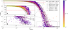 |
Fig. 1 Scaled mass of the largest remnant (Mlr/Mtot) with respect to the impact energy scaled by the catastrophic disruption criterion (QR/ |
![$\[\${\mathcal{Q}}_{\mathrm{RD}}^{*}$\]$](/articles/aa/full_html/2024/05/aa46519-23/aa46519-23-eq9.png)
2.1.1 LS12 scaling law – original fits
Equation (1), in conjunction with Eq. (2), enables the estimation of the mass of the largest post-collisional remnant, given the impact energy (![$\[\${\mathcal{Q}}_{\mathrm{RD}}^{*}$\]$](/articles/aa/full_html/2024/05/aa46519-23/aa46519-23-eq10.png) ) and the combined radius (RC1). The model incorporates three free parameters: the scaling constant, c*, the material constant,
) and the combined radius (RC1). The model incorporates three free parameters: the scaling constant, c*, the material constant, ![$\[\overline{{\mu}}\]$](/articles/aa/full_html/2024/05/aa46519-23/aa46519-23-eq11.png) , and the slope, η, for the super-catastrophic regime.
, and the slope, η, for the super-catastrophic regime.
In the original approach employed by LS12, they conducted three fits. First, using data from the works of Benz et al. (2007), Marcus et al. (2009), and Marcus et al. (2010), they estimated the catastrophic disruption criterion ![$\[\${\mathcal{Q}}_{\mathrm{RD}}^{*}$\]$](/articles/aa/full_html/2024/05/aa46519-23/aa46519-23-eq12.png) for edge-on collisions through linear interpolation of simulations with similar collision parameters. Subsequently, they fit Eq. (2) to the resulting distribution of
for edge-on collisions through linear interpolation of simulations with similar collision parameters. Subsequently, they fit Eq. (2) to the resulting distribution of ![$\[\${\mathcal{Q}}_{\mathrm{RD}}^{*}$\]$](/articles/aa/full_html/2024/05/aa46519-23/aa46519-23-eq13.png) as a function of RC1, obtaining the values: c* = 1.9 ± 0.3 and
as a function of RC1, obtaining the values: c* = 1.9 ± 0.3 and ![$\[\overline{{\mu}}\]$](/articles/aa/full_html/2024/05/aa46519-23/aa46519-23-eq14.png) = 0.36 ± 0.01 for the model parameters. Lastly, they estimated the slope η from the data points in the super-catastrophic regime (second branch of Eq. (1)). However, due to the limited number of data points in this regime, the parameter η was not well-constrained. As a result, LS12 recommended using the value η = −1.5 based on laboratory studies (Kato et al. 1995; Fujiwara et al. 1977).
= 0.36 ± 0.01 for the model parameters. Lastly, they estimated the slope η from the data points in the super-catastrophic regime (second branch of Eq. (1)). However, due to the limited number of data points in this regime, the parameter η was not well-constrained. As a result, LS12 recommended using the value η = −1.5 based on laboratory studies (Kato et al. 1995; Fujiwara et al. 1977).
2.1.2 LS12 scaling law – new fit
In contrast to the procedure implemented by LS12 of first estimating c* and ![$\[\overline{{\mu}}\]$](/articles/aa/full_html/2024/05/aa46519-23/aa46519-23-eq15.png) from the linear interpolation of
from the linear interpolation of ![$\[\${\mathcal{Q}}_{\mathrm{RD}}^{*}$\]$](/articles/aa/full_html/2024/05/aa46519-23/aa46519-23-eq16.png) and then evaluating the remaining model parameter η given QR/
and then evaluating the remaining model parameter η given QR/![$\[\${\mathcal{Q}}_{\mathrm{RD}}^{*}$\]$](/articles/aa/full_html/2024/05/aa46519-23/aa46519-23-eq17.png) and Mlr/Mtot, we decided to use the simulation data in its entirety (QR, RC1, γ, Mlr/Mtot) to directly estimate all the model parameters (c*,
and Mlr/Mtot, we decided to use the simulation data in its entirety (QR, RC1, γ, Mlr/Mtot) to directly estimate all the model parameters (c*, ![$\[\overline{{\mu}}\]$](/articles/aa/full_html/2024/05/aa46519-23/aa46519-23-eq18.png) , η) in one go. Furthermore, we introduced a new parameter, δ, that allows us to estimate the data dispersion. In particular, the dispersion is assumed to be related to the value Q/
, η) in one go. Furthermore, we introduced a new parameter, δ, that allows us to estimate the data dispersion. In particular, the dispersion is assumed to be related to the value Q/![$\[\${\mathcal{Q}}_{\mathrm{RD}}^{*}$\]$](/articles/aa/full_html/2024/05/aa46519-23/aa46519-23-eq19.png) and it is modelled, in log-space, by a normal distribution with constant standard deviation (δ). In other words, the measured value of QR/
and it is modelled, in log-space, by a normal distribution with constant standard deviation (δ). In other words, the measured value of QR/![$\[\${\mathcal{Q}}_{\mathrm{RD}}^{*}$\]$](/articles/aa/full_html/2024/05/aa46519-23/aa46519-23-eq20.png) is given by
is given by
![$\[\log\left[\frac{Q_{\mathrm{R}}}{Q_{\mathrm{RD}}^{\star}}\right]_{\mathrm{data}}=\log\left[\frac{Q_{\mathrm{R}}}{Q_{\mathrm{RD}}^{\star}}\right]_{\mathrm{model}}+N(\mu=0;\,\delta)\]$](/articles/aa/full_html/2024/05/aa46519-23/aa46519-23-eq21.png) (3)
(3)
where ![$\[\{\mathcal{N}}\]$](/articles/aa/full_html/2024/05/aa46519-23/aa46519-23-eq22.png) (μ; δ) is the normal distribution centered in μ with standard deviation δ.
(μ; δ) is the normal distribution centered in μ with standard deviation δ.
We performed a MCMC analysis with the aim of obtaining the posterior probabilities for the three model parameters plus δ as an additional free parameter. Given the dispersion model, we assumed the likelihood (![$\[\{\mathcal{L}}\]$](/articles/aa/full_html/2024/05/aa46519-23/aa46519-23-eq23.png) ) to be defined as:
) to be defined as:
![$\[\log \mathcal{L}=-\frac{N}{2} \log \left(2 \pi \delta^2\right)+\sum_i\left[\frac{\log \left(\frac{\left[Q_{\mathrm{R}} / Q_{\mathrm{RD}}^{\star}\right]_i}{\left[Q_{\mathrm{R}} / Q_{\mathrm{RD}}^{\star}\right]_{\text {model }}}\right)}{\delta}\right]^2,\]$](/articles/aa/full_html/2024/05/aa46519-23/aa46519-23-eq24.png) (4)
(4)
where the sum is over all the N data, and [QR/![$\[\${\mathcal{Q}}_{\mathrm{RD}}^{*}$\]$](/articles/aa/full_html/2024/05/aa46519-23/aa46519-23-eq25.png) ]model is obtained by inverting Eq. (1). We assumed uniform priors for all the free parameters in an wide interval around the values estimated by LS12.
]model is obtained by inverting Eq. (1). We assumed uniform priors for all the free parameters in an wide interval around the values estimated by LS12.
We ran the MCMC analysis on the entire dataset and found that the solution is strongly biased by the collisions in the merging regime (Mlr/Mtot ≳ 0.9). Among all the head-on collisions, more than a third of them have Mlr/Mtot > 0.95. This unbalance in the dataset distribution cause the MCMC to converge on a solution that favours accurate modelling of the merging regime at the expense of the remaining dataset. As evident from laboratory experiments (e.g. Takagi et al. 1984; Housen & Holsapple 1990; Nagaoka et al. 2014; Arakawa et al. 2022), the model in Eq. (1) tend to underestimate the mass of the largest remnant at very low energy. We therefore decided to exclude all the collisions with Mlr/Mtot > 0.95 from the MCMC fitting procedure.
We used uniform priors for the 4 model parameters, specifically 𝒰(0,100) for c*, 𝒰(1/3,2/3) for ![$\[\overline{{\mu}}\]$](/articles/aa/full_html/2024/05/aa46519-23/aa46519-23-eq28.png) , 𝒰(−100,0) for η, and 𝒰(0,2) for δ. Here, 𝒰(a, b) represents the uniform distribution, with a density of 1/(b – a) in the interval of a ≤ x < b and zero elsewhere. The analysis of the posteriors gives the following results: c* = 3.20 ± 0.05,
, 𝒰(−100,0) for η, and 𝒰(0,2) for δ. Here, 𝒰(a, b) represents the uniform distribution, with a density of 1/(b – a) in the interval of a ≤ x < b and zero elsewhere. The analysis of the posteriors gives the following results: c* = 3.20 ± 0.05, ![$\[\overline{{\mu}}\]$](/articles/aa/full_html/2024/05/aa46519-23/aa46519-23-eq32.png) = 0.486 ± 0.007,
= 0.486 ± 0.007, ![$\[\\eta=-11.4_{-0.8}^{+0.7}\]$](/articles/aa/full_html/2024/05/aa46519-23/aa46519-23-eq33.png) , and δ = 0.162 ± −0.003. These values differ significantly from what estimated by LS12. In particular, the slope η of the supercatastrophic regime deviates from the value −1.5 by more than 14 sigma.
, and δ = 0.162 ± −0.003. These values differ significantly from what estimated by LS12. In particular, the slope η of the supercatastrophic regime deviates from the value −1.5 by more than 14 sigma.
The value η = −1.5 suggested by LS12 was derived from two laboratory studies of collisions between solid ice (Kato et al. 1995) and collisions of polycarbonate projectiles against granite blocks (Fujiwara et al. 1977). The strong discrepancy between these laboratory fragmentation experiments and the simulations in the datasets presented here could lie in the significantly different nature of the colliding bodies more than in the methodology (simulations versus laboratory experiments). Collisions of ice and granite are in the strength regime, with the largest remnant being a single fragment of the largest body, while protoplanet collisions are in the gravity regime. This different behavior is expected to be even more evident in the catastrophic regime, where most of the colliding mass is dispersed.
The data points derived through Eq. (2) and the best fit model of Eq. (1) are shown in Fig. 1. As expected, the universal law from LS12 performs well for energies close to ![$\[\${\mathcal{Q}}_{\mathrm{RD}}^{*}$\]$](/articles/aa/full_html/2024/05/aa46519-23/aa46519-23-eq34.png) and thanks to the new estimate of η, it also succeeds in predicting the collision outcome in the super-catastrophic regime (Fig. 1B).
and thanks to the new estimate of η, it also succeeds in predicting the collision outcome in the super-catastrophic regime (Fig. 1B).
A significant discrepancy between the LS12 model and the simulations is still clearly present in the merging regime. LS12 scaling laws tend to overestimate the fragmentation efficiency for collisions with small impact energy (QR/QRD ≲ 0.3), as shown in panel A of Fig. 1. Moreover, we also noticed a strong correlation between this discrepancy and the mass ratio γ.
In Fig. 1, it is noticeable that there may be a dependence on the dataset, especially in the super-catastrophic regime (Panel B). Collisions simulated by Burger et al. (2020) and Winter et al. (2023) tend to cluster on the right-hand side of the best-fit result, indicating that more energy is required to break apart the colliding protoplanets. Conversely, collisions from the work of Timpe et al. (2020) exhibit the opposite trend. To further investigate this potential behavior, we performed separate MCMC analyses for each dataset.
We found that the parameters c* and ![$\[\overline{{\mu}}\]$](/articles/aa/full_html/2024/05/aa46519-23/aa46519-23-eq35.png) are generally in agreement across the six datasets, typically differing by less than 2σ, with only a few exceptions. Notably, the value of c* obtained from the Crespi et al. (2021) dataset, c* = 3.82 ± 0.25, exceeds the values obtained from the other datasets, which fall within the range of c* = 3.03-3.40. Additionally, the value of
are generally in agreement across the six datasets, typically differing by less than 2σ, with only a few exceptions. Notably, the value of c* obtained from the Crespi et al. (2021) dataset, c* = 3.82 ± 0.25, exceeds the values obtained from the other datasets, which fall within the range of c* = 3.03-3.40. Additionally, the value of ![$\[\overline{{\mu}}\]$](/articles/aa/full_html/2024/05/aa46519-23/aa46519-23-eq36.png) obtained from the Denman et al. (2020) dataset,
obtained from the Denman et al. (2020) dataset, ![$\[\overline{{\mu}}\]$](/articles/aa/full_html/2024/05/aa46519-23/aa46519-23-eq37.png) = 0.59 ± 0.04, surpasses the values of
= 0.59 ± 0.04, surpasses the values of ![$\[\overline{{\mu}}\]$](/articles/aa/full_html/2024/05/aa46519-23/aa46519-23-eq38.png) = 0.47+0.02−0.01 and
= 0.47+0.02−0.01 and ![$\[\overline{{\mu}}\]$](/articles/aa/full_html/2024/05/aa46519-23/aa46519-23-eq39.png) = 0.46 ± 0.02 obtained from the Timpe et al. (2020) and Burger et al. (2020) datasets, respectively.
= 0.46 ± 0.02 obtained from the Timpe et al. (2020) and Burger et al. (2020) datasets, respectively.
We observed a bimodal behavior in the parameter η, with datasets yielding either extremely low values within the range of −57 to −74 and large errors, or datasets exhibiting high values of η between −7 and −2 with smaller errors. Two prominent examples illustrating these behaviors are the Timpe et al. (2020) dataset, which yielded ![$\[\\eta=-74_{-18}^{+21}\]$](/articles/aa/full_html/2024/05/aa46519-23/aa46519-23-eq40.png) , and the Winter et al. (2023) dataset, resulting in η = −7.0 ± 0.3. Both datasets are wellsampled within the super-catastrophic regime, each comprising more than 200 datapoints. However, the Timpe et al. (2020) dataset is concentrated around Mlr/Mtot ≲ 0.1, while the Winter et al. (2023) dataset is centered around Mlr/Mtot ~ 10−3.
, and the Winter et al. (2023) dataset, resulting in η = −7.0 ± 0.3. Both datasets are wellsampled within the super-catastrophic regime, each comprising more than 200 datapoints. However, the Timpe et al. (2020) dataset is concentrated around Mlr/Mtot ≲ 0.1, while the Winter et al. (2023) dataset is centered around Mlr/Mtot ~ 10−3.
Notably, the LS12 model (Eq. (1)) enforces the fit to pass through Mlr/Mtot = 0.1 when Qr/![$\[\${\mathcal{Q}}_{\mathrm{RD}}^{*}$\]$](/articles/aa/full_html/2024/05/aa46519-23/aa46519-23-eq41.png) = 1.8, whereas the actual value is closer to Qr/Q*rd ~ 1.3. This discrepancy results in the significantly different estimates of η for the Timpe et al. (2020) and Winter et al. (2023) datasets.
= 1.8, whereas the actual value is closer to Qr/Q*rd ~ 1.3. This discrepancy results in the significantly different estimates of η for the Timpe et al. (2020) and Winter et al. (2023) datasets.
In addition, we observed varying degrees of dispersion among the different datasets, notably in simulations that incorporate the rotation of colliding protoplanets, as seen in the Timpe et al. (2020) and Winter et al. (2023) datasets. This dispersion is particularly noticeable in the super-catastrophic regime, where the presence of additional angular momentum can either aid or impede the dispersion of fragmented material.
Another distinguishing factor among the datasets arises from differences in the simulation routines and the composition of the colliding protoplanets. Nevertheless, these parameters appear to have a less significant influence compared to other collisional factors such as impact energy, relevant masses, and impact angle. An exhaustive examination of how composition affects collision outcomes falls beyond the scope of this study.
2.1.3 New scaling law
The need to model the γ-dependent offset between data and LS12 scaling laws at low impact energies, together with the pursuit of a function that smoothly transitions from the merging regime to the log-log linear super-catastrophic regime without fixing the transition point, are two pivots around which we based the new model for the universal law. A good model, able to satisfy these two requirements, is the product of an exponential function (for modelling the super-catastrophic regime) and a rational function (for modelling the merging regime). This new version of the universal law is described by
![$\[Q_{\mathrm{R}}=c_{1}Q_{\mathrm{RD}}^{\star}\left(2\frac{M_{\mathrm{lr}}}{M_{\mathrm{tot}}}\right)^{1/\eta}\frac{\left[1-\left(\frac{M_{\mathrm{lr}}}{M_{\mathrm{tot}}}\right)^{3/2}\right]^{\alpha(\gamma)}}{1+c_{2}\left(2\frac{M_{\mathrm{lr}}}{M_{\mathrm{tot}}}\right)^{2}}\,,\]$](/articles/aa/full_html/2024/05/aa46519-23/aa46519-23-eq42.png) (5)
(5)
where ![$\[\${\mathcal{Q}}_{\mathrm{RD}}^{*}$\]$](/articles/aa/full_html/2024/05/aa46519-23/aa46519-23-eq43.png) can be obtained from Eq. (2), c1 and c2 are constants and the exponent α is a function of the mass ratio γ. We observed a linear dependence between the exponent α and log γ. Therefore, we decided to model α as α(γ) = α0 + σ • log γ, where α0 and σ are two extra free parameters. We also investigated the possibility for α to depend on the combined radius RC1 but no significant correlation was found. We note that the new universal law is not analytically invertible and, in order to obtain Mlr/Mtot given (QR, γ, RC1), it would be necessarily to employ a simple root-finding algorithm.
can be obtained from Eq. (2), c1 and c2 are constants and the exponent α is a function of the mass ratio γ. We observed a linear dependence between the exponent α and log γ. Therefore, we decided to model α as α(γ) = α0 + σ • log γ, where α0 and σ are two extra free parameters. We also investigated the possibility for α to depend on the combined radius RC1 but no significant correlation was found. We note that the new universal law is not analytically invertible and, in order to obtain Mlr/Mtot given (QR, γ, RC1), it would be necessarily to employ a simple root-finding algorithm.
The model in Eq. (5) depends on three variables (QR, γ, RC1) and six parameters, two of which (c*, ![$\[\overline{{\mu}}\]$](/articles/aa/full_html/2024/05/aa46519-23/aa46519-23-eq51.png) ) arise from the physical model for
) arise from the physical model for ![$\[\${\mathcal{Q}}_{\mathrm{RD}}^{*}$\]$](/articles/aa/full_html/2024/05/aa46519-23/aa46519-23-eq52.png) (Eq. (2)) and the other five (c1, c2, η, α0, σ) arise from the new analytical model (Eq. (5)). We decided to investigate these two sets of parameters separately so that the approximation inherent to the analytical model does not affect the estimate of the physical parameters c* and
(Eq. (2)) and the other five (c1, c2, η, α0, σ) arise from the new analytical model (Eq. (5)). We decided to investigate these two sets of parameters separately so that the approximation inherent to the analytical model does not affect the estimate of the physical parameters c* and ![$\[\overline{{\mu}}\]$](/articles/aa/full_html/2024/05/aa46519-23/aa46519-23-eq53.png) .
.
To obtain the catastrophic disruption criterion (![$\[\${\mathcal{Q}}_{\mathrm{RD}}^{*}$\]$](/articles/aa/full_html/2024/05/aa46519-23/aa46519-23-eq54.png) ), we selected all the collisions with Mlr/Mtot in the range 0.4-0.6. In this neighbourhood, Mlr/Mtot scales linearly with the logarithm of the impact energy log QR with a slope of −0.97, which has been obtained by fitting the datapoints with a linear function in the semilogarithmic space. We used this linear relation to predict
), we selected all the collisions with Mlr/Mtot in the range 0.4-0.6. In this neighbourhood, Mlr/Mtot scales linearly with the logarithm of the impact energy log QR with a slope of −0.97, which has been obtained by fitting the datapoints with a linear function in the semilogarithmic space. We used this linear relation to predict ![$\[\${\mathcal{Q}}_{\mathrm{RD}}^{*}$\]$](/articles/aa/full_html/2024/05/aa46519-23/aa46519-23-eq55.png) for each collision by assuming log
for each collision by assuming log ![$\[\${\mathcal{Q}}_{\mathrm{RD}}^{*}$\]$](/articles/aa/full_html/2024/05/aa46519-23/aa46519-23-eq56.png) = log Qr - 0.97 • (Mlr/Mtot - 0.5). We note that, on average, the estimate of
= log Qr - 0.97 • (Mlr/Mtot - 0.5). We note that, on average, the estimate of ![$\[\${\mathcal{Q}}_{\mathrm{RD}}^{*}$\]$](/articles/aa/full_html/2024/05/aa46519-23/aa46519-23-eq57.png) is not affected by the chosen value for the slope since the data are homogeneously distributed around Mlr/Mtot = 0.5. In other words, a different choice of slope would only increase (or decrease) the dispersion of
is not affected by the chosen value for the slope since the data are homogeneously distributed around Mlr/Mtot = 0.5. In other words, a different choice of slope would only increase (or decrease) the dispersion of ![$\[\${\mathcal{Q}}_{\mathrm{RD}}^{*}$\]$](/articles/aa/full_html/2024/05/aa46519-23/aa46519-23-eq58.png) around the true value.
around the true value.
Finally, we used the derived values ![$\[\${\mathcal{Q}}_{\mathrm{RD}}^{*}$\]$](/articles/aa/full_html/2024/05/aa46519-23/aa46519-23-eq59.png) in the functions of RC1 and γ to determine the parameters c* and
in the functions of RC1 and γ to determine the parameters c* and ![$\[\overline{{\mu}}\]$](/articles/aa/full_html/2024/05/aa46519-23/aa46519-23-eq60.png) from Eq. (2). The analysis of the posteriors yields the following results:
from Eq. (2). The analysis of the posteriors yields the following results: ![$\[\c^*=2.661_{-0.036}^{+0.037}\]$](/articles/aa/full_html/2024/05/aa46519-23/aa46519-23-eq61.png) , and
, and ![$\[\\bar{\mu}=0.4797_{-0.0059}^{+0.0061}\]$](/articles/aa/full_html/2024/05/aa46519-23/aa46519-23-eq62.png) , with priors set to 𝒰(0,100) for c* and 𝒰(1/3,2/3) for
, with priors set to 𝒰(0,100) for c* and 𝒰(1/3,2/3) for ![$\[\overline{{\mu}}\]$](/articles/aa/full_html/2024/05/aa46519-23/aa46519-23-eq65.png) . The data and the best-fit model are presented in Fig. 2, alongside the results from LS12 for comparison.
. The data and the best-fit model are presented in Fig. 2, alongside the results from LS12 for comparison.
The new universal law (Eq. (5)) depends on five model parameters. However, the degrees of freedom can be reduced to 4 by imposing ![$\[\Q_{\mathrm{RD}}^*=\left.Q_{\mathrm{R}}\right|_{M_{\mathrm{lr}} / M_{\mathrm{tot}}=0.5}\]$](/articles/aa/full_html/2024/05/aa46519-23/aa46519-23-eq66.png) . Consequently, we can rewrite c2 as:
. Consequently, we can rewrite c2 as:
![$\[c_{2}=c_{1}\left(1-2^{-3/2}\right)^{\alpha(\gamma)}-1.]$](/articles/aa/full_html/2024/05/aa46519-23/aa46519-23-eq67.png) (6)
(6)
To obtain the remaining four parameters, we ran an MCMC algorithm, where we assumed c* = 2.661 and ![$\[\overline{{\mu}}\]$](/articles/aa/full_html/2024/05/aa46519-23/aa46519-23-eq68.png) = 0.4797. We adopted the likelihood in Eq. (4), where δ is derived by propagating the errors on c* and
= 0.4797. We adopted the likelihood in Eq. (4), where δ is derived by propagating the errors on c* and ![$\[\overline{{\mu}}\]$](/articles/aa/full_html/2024/05/aa46519-23/aa46519-23-eq69.png) . The best-fit result is displayed in Fig. 3, while the analysis of the posteriors yields the following results:
. The best-fit result is displayed in Fig. 3, while the analysis of the posteriors yields the following results: ![$\[\c_1=1.7074_{-0.0012}^{+0.0011}, \quad \eta=-10.179_{-0.022}^{+0.021}\]$](/articles/aa/full_html/2024/05/aa46519-23/aa46519-23-eq70.png) ,
, ![$\[\\alpha_0=0.1754729_{-0.00039}^{+0.00038}, \quad \sigma=-0.32516_{-0.00019}^{+0.00020}\]$](/articles/aa/full_html/2024/05/aa46519-23/aa46519-23-eq71.png) . Moreover, we estimated the data dispersion along log QR/
. Moreover, we estimated the data dispersion along log QR/![$\[\${\mathcal{Q}}_{\mathrm{RD}}^{*}$\]$](/articles/aa/full_html/2024/05/aa46519-23/aa46519-23-eq72.png) and we obtained an approximately constant and symmetric dispersion of 0.11. The dispersion is attributed to various factors not considered in our model, including (but not limited to) the chemical composition of the colliding bodies, their rotation, and the angular momentum of the collision. For the MCMC analysis, we used the following priors for the fit parameters: 𝒰(0, 100) for c1, 𝒰(−100,0) for η, 𝒰(0,10) for α0, and 𝒰(−10,0) for σ. The best fit parameters for our new model, together with the values from LS12 model, are summarised in Table 2
and we obtained an approximately constant and symmetric dispersion of 0.11. The dispersion is attributed to various factors not considered in our model, including (but not limited to) the chemical composition of the colliding bodies, their rotation, and the angular momentum of the collision. For the MCMC analysis, we used the following priors for the fit parameters: 𝒰(0, 100) for c1, 𝒰(−100,0) for η, 𝒰(0,10) for α0, and 𝒰(−10,0) for σ. The best fit parameters for our new model, together with the values from LS12 model, are summarised in Table 2
We noted that the new universal law is asymptotic for Mlr/Mtot → 1. This behaviour is nonphysical and approximations must be employed. From the MCMC analysis, we obtained that our model starts deviating from the measured values of QR/![$\[\${\mathcal{Q}}_{\mathrm{RD}}^{*}$\]$](/articles/aa/full_html/2024/05/aa46519-23/aa46519-23-eq77.png) when Mlr/Mtot > 0.999. We propose assuming the collisions in this regime to be the perfect merging of the two bodies (Mlr/Mtot = 1).
when Mlr/Mtot > 0.999. We propose assuming the collisions in this regime to be the perfect merging of the two bodies (Mlr/Mtot = 1).
Following the approach outlined in the previous section, we conducted a separate analysis of the datasets. Generally, the results from different datasets exhibit consistency, and any observed discrepancies can be attributed to the differences between the datasets as described in Sect. 2.1.2. The most notable deviation was observed in the dataset from Denman et al. (2020). In the case of this specific dataset, we observed that our model tends to overestimate the mass of the largest remnant during merging events (panel A of Fig. 3). This deviation can be attributed to the presence of an atmosphere in the Denman et al. (2020) dataset, a feature absent in the other datasets we considered
As noted by Denman et al. (2020), low-energy impacts primarily result in atmosphere loss, while more energetic impacts are required to fragment both the mantle and the core of the colliding bodies. Therefore, caution should be exercised when applying our model to collisions involving planets with a substantial atmosphere, as it may not accurately represent the outcomes in such scenarios.
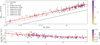 |
Fig. 2 Catastrophic disruption criterion for same-mass collisions ( |
![$\[\{\mathcal{Q}}_{\mathrm{RD,\gamma=1}}^{*}\]$](/articles/aa/full_html/2024/05/aa46519-23/aa46519-23-eq44.png)
![$\[\{\mathcal{Q}}_{\mathrm{RD,\gamma=1}}^{*}\]$](/articles/aa/full_html/2024/05/aa46519-23/aa46519-23-eq45.png)
![$\[\${\mathcal{Q}}_{\mathrm{RD}}^{*}$\]$](/articles/aa/full_html/2024/05/aa46519-23/aa46519-23-eq46.png)
![$\[\left[(1+\gamma)^{2}/4\gamma\right]^{2/(3\bar{\mu})-1}\]$](/articles/aa/full_html/2024/05/aa46519-23/aa46519-23-eq47.png)
![$\[\Q_{\mathrm{RD},\gamma=1}^{\star}/R_{\mathrm{Cl}}^{2}\]$](/articles/aa/full_html/2024/05/aa46519-23/aa46519-23-eq48.png)
![$\[\overline{{\mu}}\]$](/articles/aa/full_html/2024/05/aa46519-23/aa46519-23-eq49.png)
![$\[\overline{{\mu}}\]$](/articles/aa/full_html/2024/05/aa46519-23/aa46519-23-eq50.png)
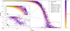 |
Fig. 3 Scaled mass of the largest remnant (Mlr/Mtot) with respect to the impact energy scaled by the catastrophic disruption criterion (QR/ |
![$\[\${\mathcal{Q}}_{\mathrm{RD}}^{*}$\]$](/articles/aa/full_html/2024/05/aa46519-23/aa46519-23-eq78.png)
Best fit parameters and associated error.
2.2 Models comparison
Here, we compare the performance of three different models: the analytical model from LS12 with the new best-fit parameters, the new analytical model presented in this work, and a simple machine learning (ML) model to provide a benchmark against which to compare our new analytical model. We thus trained a classic Random Forest Regressor (Pedregosa et al. 2011) using its default hyperparameters and three features only: the impact energy (QR), the combined radius (RC1), and the mass ratio (γ). We also limited the dataset to the head-on collision cases.
The predicted values from the ML model, as well as the original data, are depicted in Fig. 4, compared to the original model from LS12 (Sec. 4) and the new model introduced in this study (Sect. 2.1.3).
We observe that the ML model effectively captures the dispersion around the mean of the predicted quantity, a characteristic not readily attainable with analytical models. However, it is worth noting that in the super catastrophic regime, we observe deviations in the predicted outcomes from the ML model, especially in cases involving high rotators from the Timpe et al. (2020) dataset. This discrepancy may be attributed to the limited number of parameters on which the ML model has been trained.
Introducing rotation as a parameter in the ML model could potentially enhance its predictive efficiency. Nevertheless, this falls outside the scope of our current study, which is primarily focused on evaluating and comparing the predictive capabilities of our analytical model against those of a ML model that operates without relying on analytical assumptions.
Quantitatively, metric scores for the different models are summarized in Table 3. We calculated the root mean squared error (RMSE) of (y, ŷ) ![$\[\(y,{\hat{y}})\,=\,{\sqrt{\frac{\sum_{i=0}^{N-1}(y_{i}-{\hat{y}}_{i})^{2}}{N}}}\]$](/articles/aa/full_html/2024/05/aa46519-23/aa46519-23-eq81.png) along with the median absolute error,
along with the median absolute error,
![$\[{\mathrm{med~abs~err}}(y,{\hat{y}})={\mathrm{median}}(\vert y_{1}-{\hat{y}}_{1}\vert,\dots,\vert y_{n}-{\hat{y}}_{n}\vert)\]$](/articles/aa/full_html/2024/05/aa46519-23/aa46519-23-eq82.png)
![$\[{\mathrm{med.~rel~err}}(y,{\hat{y}})={\mathrm{median}}(|\,y_{1}-{\hat{y}}_{1}\ |\,/\,|\,y_{1}\ |,\ldots,|\,y_{n}-{\hat{y}}_{n}\ |\,/\,|\,y_{n}\,|)\]$](/articles/aa/full_html/2024/05/aa46519-23/aa46519-23-eq83.png)
between the actual and predicted scaled mass of the largest remnant. We find that while the three models have comparable root mean squared errors as this metric is dominated by large Mlr/Mtot values, the new analytical model outperforms LS12 by factors of (respectively) ~6 and 4 on the more sensitive median absolute and relative errors. The errors of the ML model, taken as the average of a 10-fold cross-validation, are all very close to our new analytical model, reflecting the fact that complex models are not needed for simple low dimensionality problems.
Retraining the model using all the available parameters, such as the mass the composition and the spin of the colliding bodies, did not significantly improve its overall performance for head-on cases. This result confirms that the collision outcome is strongly dependent on the three parameters used in the scaling laws.
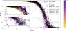 |
Fig. 4 Scaled mass of the largest remnant (Mlr/Mtot) with respect to the impact energy scaled by the catastrophic disruption criterion (QR/ |
![$\[\${\mathcal{Q}}_{\mathrm{RD}}^{*}$\]$](/articles/aa/full_html/2024/05/aa46519-23/aa46519-23-eq80.png)
Accuracy metrics to compare the analytical models of LS12 and this work, in addition to our restricted ML model.
3 Summary and conclusions
3.1 LS12 scaling laws compared to new data
In this work, we review the two main analytical models that the widely used scaling laws from Leinhardt & Stewart (2012) are founded, on, namely: the catastrophic disruption criterion, which allows us to estimate the collision energy needed to disperse half of the total mass involved in the collision, and the universal law, which allows us to predict the mass of the largest post–collisional remnant (Mlr/Mtot). We used six datasets of SPH simulations of collisions from the works of Burger et al. (2020), Denman et al. (2020), Gabriel et al. (2020), Timpe et al. (2020), Crespi et al. (2021), and Winter et al. (2023), for a total of more than 32000 simulations.
By comparing the LS12 scaling laws with the new datasets we observed that these laws tend to underestimate the mass of the largest remnant in the accretion regime (Mlr/Mtot ≳ 0.9). In this regime, we also noticed a strong dependence between Mlr/Mtot and the mass ratio of the colliding bodies (γ). In particular, collisions with the same scaled impact energy (QR/![$\[\${\mathcal{Q}}_{\mathrm{RD}}^{*}$\]$](/articles/aa/full_html/2024/05/aa46519-23/aa46519-23-eq84.png) ) but a smaller mass ratio of the colliding bodies tend to result in a less efficient accretion and merger than collisions with a larger mass ratio. In the catastrophic regime (Mlr/Mtot ≳ 0.9), we observed a strong discrepancy between LS12 scaling laws and our dataset. In particular, we obtained a slope of η = −11.4+0.7−0.8 when fitting the LS12 model to our dataset, compared to η = −1.2 ~ −1.5 predicted by LS12.
) but a smaller mass ratio of the colliding bodies tend to result in a less efficient accretion and merger than collisions with a larger mass ratio. In the catastrophic regime (Mlr/Mtot ≳ 0.9), we observed a strong discrepancy between LS12 scaling laws and our dataset. In particular, we obtained a slope of η = −11.4+0.7−0.8 when fitting the LS12 model to our dataset, compared to η = −1.2 ~ −1.5 predicted by LS12.
3.2 New scaling laws
We developed an analytical scaling law that, analogously to the universal law from LS12, can be used to predict the mass of the largest remnant of a collision between gravity-dominated bodies. Our model (Eq. (5)) is able to reproduce the γ-dependent distribution observed in the accretive regime, as well as exponential decrease in the catastrophic regime. It is valid for MlrMtot < 0.999, beyond which we suggest assuming that the collision resulted in an inelastic merger. Following the work of LS12, we assumed the catastrophic disruption criterion in the gravity regime to be modeled by Eq. (2), and we found best-fit parameters ![$\[\c^*=2.661_{-0.036}^{+0.037}\]$](/articles/aa/full_html/2024/05/aa46519-23/aa46519-23-eq85.png) , and
, and ![$\[\\bar{\mu}=0.4797_{-0.0059}^{+0.0061}\]$](/articles/aa/full_html/2024/05/aa46519-23/aa46519-23-eq86.png) . LS12 estimated these two parameters to be c* = 1.9 ± 0.3,
. LS12 estimated these two parameters to be c* = 1.9 ± 0.3, ![$\[\overline{{\mu}}\]$](/articles/aa/full_html/2024/05/aa46519-23/aa46519-23-eq87.png) = 0.36 ± 0.01. Our estimate for the offset parameter c* is at the border of compatibility with what was obtained by LS12. However, it is interesting to notice that LS12 estimate with a value that is 30% smaller than what we observed, results in a more efficient fragmentation of the main colliding body and, therefore, an overestimation of the debris production. The
= 0.36 ± 0.01. Our estimate for the offset parameter c* is at the border of compatibility with what was obtained by LS12. However, it is interesting to notice that LS12 estimate with a value that is 30% smaller than what we observed, results in a more efficient fragmentation of the main colliding body and, therefore, an overestimation of the debris production. The ![$\[\overline{{\mu}}\]$](/articles/aa/full_html/2024/05/aa46519-23/aa46519-23-eq88.png) value obtained by LS12 is indicative of almost pure momentum scaling for gravity–dominated bodies, while our value suggests a balanced combination between momentum and energy coupling. However, caution must be practiced when deriving any significant physical conclusion about the energy-momentum coupling since both LS12 and our estimate of
value obtained by LS12 is indicative of almost pure momentum scaling for gravity–dominated bodies, while our value suggests a balanced combination between momentum and energy coupling. However, caution must be practiced when deriving any significant physical conclusion about the energy-momentum coupling since both LS12 and our estimate of ![$\[\overline{{\mu}}\]$](/articles/aa/full_html/2024/05/aa46519-23/aa46519-23-eq89.png) fit well inside the data dispersion (see Fig. 2). Finally, we found that ML models such as the Random Forest Regressor do not perform better than the new analytical model, confirming the prediction efficiency of the latter.
fit well inside the data dispersion (see Fig. 2). Finally, we found that ML models such as the Random Forest Regressor do not perform better than the new analytical model, confirming the prediction efficiency of the latter.
Acknowledgements
We would like to express our gratitude to Christoph Schäfer for his valuable comments and feedback on this manuscript. His suggestions and criticism have greatly improved the quality of our work. This material is based upon work supported by Tamkeen under the NYU Abu Dhabi Research Institute grant CASS.
References
- Arakawa, M., Okazaki, M., Nakamura, M., et al. 2022, Icarus, 373, 114777 [NASA ADS] [CrossRef] [Google Scholar]
- Benz, W. 1990, in Numerical Modelling of Nonlinear Stellar Pulsations Problems and Prospects, ed. J. R. Buchler, 269 [Google Scholar]
- Benz, W., Anic, A., Horner, J., & Whitby, J. A. 2007, Space Sci. Rev., 132, 189 [CrossRef] [Google Scholar]
- Burger, C., Maindl, T. I., & Schäfer, C. M. 2018, Celest. Mech. Dyn. Astron., 130, 2 [NASA ADS] [CrossRef] [Google Scholar]
- Burger, C., Bazsó, Á., & Schäfer, C. M. 2020, A&A, 634, A76 [NASA ADS] [CrossRef] [EDP Sciences] [Google Scholar]
- Chambers, J. E. 1999, MNRAS, 304, 793 [Google Scholar]
- Chambers, J. E. 2001, Icarus, 152, 205 [Google Scholar]
- Chambers, J. E. 2013, Icarus, 224, 43 [CrossRef] [Google Scholar]
- Chambers, J. E., & Wetherill, G. W. 1998, Icarus, 136, 304 [NASA ADS] [CrossRef] [Google Scholar]
- Chau, A., Reinhardt, C., Helled, R., & Stadel, J. 2018, ApJ, 865, 35 [NASA ADS] [CrossRef] [Google Scholar]
- Clement, M. S., Kaib, N. A., Raymond, S. N., Chambers, J. E., & Walsh, K. J. 2019a, Icarus, 321, 778 [NASA ADS] [CrossRef] [Google Scholar]
- Clement, M. S., Raymond, S. N., & Kaib, N. A. 2019b, AJ, 157, 38 [NASA ADS] [CrossRef] [Google Scholar]
- Clement, M. S., Quintana, E. V., & Quarles, B. L. 2022, ApJ, 928, 91 [NASA ADS] [CrossRef] [Google Scholar]
- Crespi, S., Dobbs-Dixon, I., Georgakarakos, N., et al. 2021, MNRAS, 508, 6013 [NASA ADS] [CrossRef] [Google Scholar]
- Denman, T. R., Leinhardt, Z. M., Carter, P. J., & Mordasini, C. 2020, MNRAS, 496, 1166 [NASA ADS] [CrossRef] [Google Scholar]
- Duncan, M. J., Levison, H. F., & Lee, M. H. 1998, AJ, 116, 2067 [Google Scholar]
- Emsenhuber, A., Jutzi, M., & Benz, W. 2018, Icarus, 301, 247 [NASA ADS] [CrossRef] [Google Scholar]
- Esteves, L., Izidoro, A., Bitsch, B., et al. 2022, MNRAS, 509, 2856 [Google Scholar]
- Fujiwara, A., Kamimoto, G., & Tsukamoto, A. 1977, Icarus, 31, 277 [NASA ADS] [CrossRef] [Google Scholar]
- Gabriel, T. S. J., Jackson, A. P., Asphaug, E., et al. 2020, ApJ, 892, 40 [NASA ADS] [CrossRef] [Google Scholar]
- Holsapple, K., Giblin, I., Housen, K., Nakamura, A., & Ryan, E. 2002, in Asteroids III, 443 [CrossRef] [Google Scholar]
- Housen, K. R., & Holsapple, K. A. 1990, Icarus, 84, 226 [NASA ADS] [CrossRef] [Google Scholar]
- Housen, K. R., & Holsapple, K. A. 1999, Icarus, 142, 21 [NASA ADS] [CrossRef] [Google Scholar]
- Ishigaki, Y., Kominami, J., Makino, J., Fujimoto, M., & Iwasawa, M. 2021, PASJ, 73, 660 [NASA ADS] [CrossRef] [Google Scholar]
- Izidoro, A., Ogihara, M., Raymond, S. N., et al. 2017, MNRAS, 470, 1750 [Google Scholar]
- Kato, M., Iijima, Y.-I., Arakawa, M., et al. 1995, Icarus, 113, 423 [NASA ADS] [CrossRef] [Google Scholar]
- Kegerreis, J. A., Eke, V. R., Catling, D. C., et al. 2020, ApJ, 901, L31 [NASA ADS] [CrossRef] [Google Scholar]
- Kokubo, E., & Genda, H. 2010, ApJ, 714, L21 [Google Scholar]
- Kokubo, E., & Ida, S. 1996, Icarus, 123, 180 [Google Scholar]
- Leinhardt, Z. M., & Stewart, S. T. 2012, ApJ, 745, 79 [NASA ADS] [CrossRef] [Google Scholar]
- Leinhardt, Z. M., Richardson, D. C., & Quinn, T. 2000, Icarus, 146, 133 [NASA ADS] [CrossRef] [Google Scholar]
- Leinhardt, Z. M., Richardson, D. C., Lufkin, G., & Haseltine, J. 2009, MNRAS, 396, 718 [CrossRef] [Google Scholar]
- Leinhardt, Z. M., Dobinson, J., Carter, P. J., & Lines, S. 2015, ApJ, 806, 23 [NASA ADS] [CrossRef] [Google Scholar]
- Marcus, R. A., Stewart, S. T., Sasselov, D., & Hernquist, L. 2009, ApJ, 700, L118 [CrossRef] [Google Scholar]
- Marcus, R. A., Sasselov, D., Stewart, S. T., & Hernquist, L. 2010, ApJ, 719, L45 [NASA ADS] [CrossRef] [Google Scholar]
- Melosh, H. J. 2007, Meteor. Planet. Sci., 42, 2079 [NASA ADS] [CrossRef] [Google Scholar]
- Monaghan, J. J. 1992, ARA&A, 30, 543 [NASA ADS] [CrossRef] [Google Scholar]
- Mustill, A. J., Davies, M. B., & Johansen, A. 2018, MNRAS, 478, 2896 [NASA ADS] [CrossRef] [Google Scholar]
- Nagaoka, H., Takasawa, S., Nakamura, A. M., & Sangen, K. 2014, Meteor. Planet. Sci., 49, 69 [NASA ADS] [CrossRef] [Google Scholar]
- O'Brien, D. P., Morbidelli, A., & Levison, H. F. 2006, Icarus, 184, 39 [CrossRef] [Google Scholar]
- Pedregosa, F., Varoquaux, G., Gramfort, A., et al. 2011, J. Mach. Learn. Res., 12, 2825 [Google Scholar]
- Poon, S. T. S., Nelson, R. P., Jacobson, S. A., & Morbidelli, A. 2020, MNRAS, 491, 5595 [Google Scholar]
- Quintana, E. V., Lissauer, J. J., Chambers, J. E., & Duncan, M. J. 2002, ApJ, 576, 982 [NASA ADS] [CrossRef] [Google Scholar]
- Quintana, E. V., Barclay, T., Borucki, W. J., Rowe, J. F., & Chambers, J. E. 2016, ApJ, 821, 126 [NASA ADS] [CrossRef] [Google Scholar]
- Raymond, S. N., Quinn, T., & Lunine, J. I. 2004, Icarus, 168, 1 [NASA ADS] [CrossRef] [Google Scholar]
- Raymond, S. N., Quinn, T., & Lunine, J. I. 2006, Icarus, 183, 265 [Google Scholar]
- Reinhardt, C., Chau, A., Stadel, J., & Helled, R. 2020, MNRAS, 492, 5336 [NASA ADS] [CrossRef] [Google Scholar]
- Reufer, A. 2011, Ph.D. Thesis, University of Bern, Switzerland [Google Scholar]
- Schäfer, C., Riecker, S., Maindl, T. I., et al. 2016, A&A, 590, A19 [NASA ADS] [CrossRef] [EDP Sciences] [Google Scholar]
- Schäfer, C. M., Wandel, O. J., Burger, C., et al. 2020, Astron. Comput., 33, 100410 [CrossRef] [Google Scholar]
- Springel, V. 2005, MNRAS, 364, 1105 [Google Scholar]
- Stewart, S. T., & Leinhardt, Z. M. 2009, ApJ, 691, L133 [NASA ADS] [CrossRef] [Google Scholar]
- Takagi, Y., Mizutani, H., & Kawakami, S.-I. 1984, Icarus, 59, 462 [NASA ADS] [CrossRef] [Google Scholar]
- Thompson, S. L., & Lauson, H. S. 1972, Improvements in the Chart D Radiation-Hydrodynamic Code. III: Revised Analytic Equations of State (Albuquerque, New Mexico: Sandia National Laboratory), Technical Report SC-RR-71-0714 [Google Scholar]
- Tillotson, J. H. 1962, Metallic Equations of State For Hypervelocity Impact, General Atomic Report GA-3216, Technical Report [Google Scholar]
- Timpe, M. L., Han Veiga, M., Knabenhans, M., Stadel, J., & Marelli, S. 2020, Computat. Astrophys. Cosmol., 7, 2 [NASA ADS] [CrossRef] [Google Scholar]
- Wadsley, J. W., Stadel, J., & Quinn, T. 2004, New Astron. 9, 137 [Google Scholar]
- Wallace, J., Tremaine, S., & Chambers, J. 2017, AJ, 154, 175 [NASA ADS] [CrossRef] [Google Scholar]
- Wetherill, G. W. 1980, ARA&A, 18, 77 [NASA ADS] [CrossRef] [Google Scholar]
- Wetherill, G. W. 1994, Geochim. Cosmochim. Acta, 58, 4513 [NASA ADS] [CrossRef] [Google Scholar]
- Winter, P. M., Burger, C., Lehner, S., et al. 2023, MNRAS, 520, 1224 [NASA ADS] [CrossRef] [Google Scholar]
For more details about smooth particle hydrodynamics (SPH) simulations we refer the reader to the works of Benz (1990) and Monaghan (1992).
All Tables
Three catalogues used in this study (top) and catalogues used in LS12 for gravity-dominated bodies (bottom).
Accuracy metrics to compare the analytical models of LS12 and this work, in addition to our restricted ML model.
All Figures
|
Fig. 1 Scaled mass of the largest remnant (Mlr/Mtot) with respect to the impact energy scaled by the catastrophic disruption criterion (QR/ |
| In the text | |
|
Fig. 2 Catastrophic disruption criterion for same-mass collisions ( |
| In the text | |
|
Fig. 3 Scaled mass of the largest remnant (Mlr/Mtot) with respect to the impact energy scaled by the catastrophic disruption criterion (QR/ |
| In the text | |
|
Fig. 4 Scaled mass of the largest remnant (Mlr/Mtot) with respect to the impact energy scaled by the catastrophic disruption criterion (QR/ |
| In the text | |
Current usage metrics show cumulative count of Article Views (full-text article views including HTML views, PDF and ePub downloads, according to the available data) and Abstracts Views on Vision4Press platform.
Data correspond to usage on the plateform after 2015. The current usage metrics is available 48-96 hours after online publication and is updated daily on week days.
Initial download of the metrics may take a while.