| Issue |
A&A
Volume 620, December 2018
|
|
|---|---|---|
| Article Number | A101 | |
| Number of page(s) | 15 | |
| Section | Celestial mechanics and astrometry | |
| DOI | https://doi.org/10.1051/0004-6361/201833197 | |
| Published online | 05 December 2018 | |
Optimizing asteroid orbit computation for Gaia with normal points
1
Department of Physics, Gustaf Hällströmin katu 2a, University of Helsinki, PO Box 64, 00014 Finland
e-mail: fedorets@iki.fi
2
Nordic Optical Telescope, Rambla José Ana Fernández Perez 7, Local 5, 38711 Breña Baja, La Palma, Santa Cruz de Tenerife, Spain
3
Finnish Geospatial Research Institute, Geodeetinrinne 2, 02340 Masala, Finland
4
Observatoire Royal de Belgique, Avenue Circulaire 3, 1180 Bruxelles, Belgium
5
Department of Computer Science, Electrical and Space Engineering, Luleå University of Technology, Box 848, 98128 Kiruna, Sweden
6
Université Côte d’Azur, Observatoire de la Côte d’Azur, CNRS, Laboratoire Lagrange, Boulevard de l’Observatoire, CS34229, 06304 Nice Cedex 4, France
7
IMCCE, Institut de Mécanique Céleste et de Calcul des Éphémérides, Observatoire de Paris, PSL Research University, CNRS-UMR8028, Sorbonne Universités, UPMC Univ. Paris 06, Université de Lille, 77 avenue Denfert-Rochereau, 75014 Paris, France
8
INAF, Osservatorio Astrofisico di Arcetri, Largo Enrico Fermi 5, 50125 Firenze, Italy
9
Observatoire de Besançon, UMR CNRS 6213, 41 bis avenue de l’Observatoire, 25000 Besançon, France
Received:
9
April
2018
Accepted:
12
October
2018
Context. In addition to the systematic observations of known solar-system objects (SSOs), a continuous processing of new discoveries requiring fast responses is implemented as the short-term processing of Gaia SSO observations, providing alerts for ground-based follow-up observers. The common independent observation approach for the purposes of orbit computation has led to unrealistically large ephemeris prediction uncertainties when processing real Gaia data.
Aims. We aim to provide ground-based observers with a cloud of sky positions that is shrunk to a fraction of the previously expected search area by making use of the characteristic features of Gaia astrometry. This enhances the efficiency of Gaia SSO follow-up network and leads to an increased rate of asteroid discoveries with reasonably constrained orbits with the help of ground-based follow-up observations of Gaia asteroids.
Methods. We took advantage of the separation of positional errors of Gaia SSO observations into a random and systematic component. We treated the Gaia observations in an alternative way by collapsing up to ten observations that correspond to a single transit into a single so-called normal point. We implemented this input procedure in the Gaia SSO short-term processing pipeline and the OpenOrb software.
Results. We validate our approach by performing extensive comparisons between the independent observation and normal point input methods and compare them to the observed positions of previously known asteroids. The new approach reduces the ephemeris uncertainty by a factor of between three and ten compared to the situation where each point is treated as a separate observation.
Conclusions. Our new data treatment improves the sky prediction for the Gaia SSO observations by removing low-weight orbital solutions. These solutions originate from excessive curvature of observations, introduced by short-term variations of Gaia attitude on the one hand, and, as a main effect, shrinking of systematic error bars in the independent observation case on the other hand. We anticipate that a similar approach may also be utilized in a situation where observations from a single observatory dominate.
Key words: astrometry / celestial mechanics / minor planets / asteroids: general
© ESO 2018
1. Introduction
As of 2018, ESA’s astrometric cornerstone mission Gaia, is in constant whole-sky scanning operation mode (Gaia Collaboration 2016). Primarily focusing on stellar astrometry with unprecedented precision and coverage, Gaia also contributes substantially to asteroid science (e.g. Mignard et al. 2007; Tanga et al. 2016). The primary contribution of Gaia to solar system research is very-high precision astrometry of known solar-system objects (SSOs), distributed with Gaia data releases, and calibrated with use of Gaia’s subsequent iterative reference frames (e.g. Gaia Collaboration 2018a). The first distribution of Gaia SSO data occurred as part of Gaia Data Release 2, and is described by Gaia Collaboration (2018b).
In addition to providing high-precision astrometry of known SSOs, Gaia also has the potential to enable discovery of new asteroids1 (Mignard et al. 2007; Carry 2014). The particular strength of Gaia is its whole-sky coverage, which permits discovery of asteroids from under-represented off-ecliptic areas. Another strength is that due to its observational geometry, Gaia has the potential to enable discovery of asteroids interior to the Earth’s orbit (the so-called Atira asteroids). Only 12 Atiras are currently known out of potentially thousands of observable objects (Ribeiro et al. 2016; Granvik et al. 2018). We note that while having a spaceborne advantage, Gaia is not the only survey instrument capable of discovering off-ecliptic asteroids. For the southern hemisphere, for example, mining the Kilo-Degree Survey (KiDS; Mahlke et al. 2018) also provides off-ecliptic asteroid astrometry. In the case of potential asteroid discoveries, the available positional data and errors are of “quick-look” quality (unlike for the iterative solutions of Gaia data releases), and follow-up observations are urgently required. The required quick response time comes at the expense of reduced calibration data quality.
An astrometric Gaia observation of an SSO is recorded on an array of consecutive charge-coupled devices (CCDs) – the sky mapper, which detects the object, and nine astrometric fields, which monitor the sky position and motion of the object. Two additional CCDs – the blue and red photometers – do not contribute to astrometry. Initially, the two recorded positions are along-scan and across-scan, with respect to Gaia’s on-sky movement. The across-scan position is constrained worse (Gaia Collaboration 2018b), and in case of the short-term processing is only extractable from the single sky mapper position. A set of observations forms a “transit”, which typically includes from four to ten observations. The number of observations depends on the initial placement of the asteroid on the across-scan direction and its spatial velocity. The maximum duration of each transit is 50 s. The transits are then cross-correlated linearly to produce collections of transits known as “bundles”. These bundles are then used as an input for asteroid orbital inversion. The orbital inversion produces a set of orbits that reproduce the observed positions to within the expected uncertainties by using random-walk statistical ranging (Muinonen et al. 2016). This pipeline is run on a daily basis at the Data Processing Centre CNES (DPCC, Toulouse, France). The orbital solutions not corresponding to any known SSOs identified previously in the workflow are treated as new asteroid candidates, and are fed to the follow-up network (FUN) software. In the follow-up network software, SSO orbits are propagated to ephemerides for a set of different epochs, and these are then dispatched to ground-based observers via a web-based tool. The follow-up observations are coordinated at the Institut de mécanique céleste et de calcul des éphémérides (IMCCE, Observatoire de Paris, France).
In an effort to discover new asteroids, a daily processing chain of Gaia asteroid data has been established (Tanga et al. 2016) within the Gaia Data Processing and Analysis Consortium (DPAC). Due to Gaia’s permanent scanning drift on the one hand and the sky motion of asteroids on the other hand, Gaia is capable of observing a moving object for only a short duration at a time, typically from four hours to two days. It is expected that Gaia will observe each known asteroid between 60 and 70 times during its nominal five-year operational phase (Mignard et al. 2007). Although the errors are of the milliarcsecond order, classical optimization and minimization methods (such as least-squares methods) are not sufficient enough for future positional predictions for newly discovered SSOs due to very short observational arcs. Instead, it is advantageous to use statistical sampling-based orbital inversion methods, in other words, to find all the possible orbital solutions for a given set of observations within the given uncertainties.
However, upon discovery, the swarm of proposed orbits does not converge in the phase space of Keplerian orbital elements which would allow well-constrained ephemerides to be computed for topocentric follow-up observers (Muinonen et al. 2016). DPAC’s daily processing of SSOs aims to provide alerts for ground-based observers to carry out astrometric observations that constrain the orbits of asteroids recently discovered by Gaia (Thuillot et al. 2014) before the discovered SSOs are lost. New discoveries are concentrated towards the faint end of Gaia’s detection capabilities, i.e. G> 20. Here and henceforth G refers to the intrinsic Gaia white-light magnitude Jordi et al. (2010).
The initial results of the short-term processing yielded unexpectedly large search areas for follow-up observations of candidate asteroids. The sky areas proved to be much larger than was expected from results obtained with the simulation data. Also, the predicted sky areas for recoveries, typically comprising areas of over one square degree directly after processing, were deemed too large to be realistically covered by follow-up observers in a reasonable amount of time. Therefore it was necessary to take measures to narrow the search region. In case of short-term processing, systematic errors are typically of the same order of magnitude as random errors. A proper way for dealing with systematic errors in orbit computation (which is the most probable source for such large search areas) had to be developed. As Gaia has a distinct operational mode with clear discrepancies in its along-scan and across-scan directions, the detection of movement by subsequent CCDs, and the inapplicability of postfit statistical analysis of astrometric uncertainties due to existing estimates, direct methods for accounting weights between different observatories and star catalogues (Carpino et al. 2003; Chesley et al. 2010; Baer et al. 2011; Farnocchia et al. 2015a; Vereš et al. 2017) are not applicable. The error model of Gaia transits and the internal correlations of points within a single transit thus needed to be re-assessed.
In the current work, we present a method to improve initial asteroid computation by taking into account the systematic and random errors of Gaia observations at the orbital inversion phase of the data processing chain. The numerical methods are described in Sect. 2, computational results in Sect. 3, and conclusions in Sect. 4.
2. Asteroid orbital inversion
2.1. Error model
The various sources of uncertainty have been identified at the inter-CCD threading step. Understanding the error model is essential for improving the treatment of the input data. We note that the error model in the short-term processing is different from the long-term processing (Gaia Collaboration 2018b). In the short-term, the data needs to be delivered quickly to the follow-up observers, thus the Gaia attitude used cannot be iteratively calibrated.
The within-transit systematic error includes contributions (in order of significance) from Gaia’s attitude, light bending, relativistic aberration and the photocentre shift (Muinonen & Lumme 2015) of the observed objects. The inherent feature of nearly-daily processing of data is the fact that the attitude used for asteroid alerts is a single-day approximation, which is several orders of magnitude worse than the accuracy produced for Gaia releases. The 1σ-uncertainty for this one-day attitude is rather constant, being of the order of 70–80 mas, and is the main contributor to the overall error budget.
The major contributor for the within-transit random error is the location of the geometric centre of the object in Gaia’s across-scan direction. Smaller contributors to the random-error are the geometric centre in the along-scan direction and Gaia’s attitude.
The true single-day Gaia attitude must be calculated from two auxiliary Gaia attitudes. One of these is responsible for the stable direction while the other provides the position information. The variations of the position-providing attitude are of the order of the duration of a single transit in the short-term processing. As a result, the asteroid positions mirror the short-term attitude variations. The schematic of the movement of the asteroid in the short-term procesing is presented in Fig. 1.
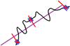 |
Fig. 1. Along-scan position of an asteroid as a function of time in Gaia short-term processing. The purple line depicts the true position of the asteroid, and the black line depicts the position suffering systematically from the uncertainties in the Gaia attitude model. Blue bars describe observations and their random errors grouped in transits, red points are normal points, and red lines are systematic errors. The treatment of the across-scan position is analogous. |
Gaia asteroid observations suffer somewhat from the fact that although the measurement of an object’s position is very precise in Gaia’s along-scan direction (submilliarcsecond accuracy at best) for astrometric field CCDs, the across-scan direction is significantly less accurate for G > 13. The only across-scan information is extracted from the star-mapper CCD, but it has proven to often fail to converge with other observations in the linear fit produced at the astrometric reduction step. Two identified reasons for the worse position values from the star mapper are bad calibration and additional binning of the CCD, further reducing the accuracy.
It has been decided that the positions provided by the star mapper would be completely omitted in the long-term processing of Gaia asteroid orbits. For short-term processing they are retained at the possible cost of including outliers because they are the only source of positional information in across-scan direction, apart from the fact that we know that the object is inside the transmitted window in the astrometric field CCDs.
As a result, a number of different effects plays a role in deteriorating the ephemeris predictions of the short-term processing. These effects, and the introduced improvements of the new data model is discussed in Sect. 3.
2.2. Orbital-element probability density
We describe the six osculating orbital elements of an asteroid at a given epoch t0 (the epoch of the first observation) by the vector P. For Keplerian orbital elements, P = (a, e, i, Ω, ω, M0)T (T is transpose) and the elements are, respectively, the semi-major axis, eccentricity, inclination, longitude of ascending node, argument of perihelion, and the mean anomaly at t0. The angular elements i, Ω, and ω are referred to the ecliptic at equinox J2000.0. For Cartesian elements, P = (X, Y, Z, Ẋ, Ẏ, Ż)T, where, in a given reference frame at t0, the vectors (X, Y, Z)T and (Ẋ, Ẏ, Ż)T denote the position and velocity, respectively.
We start with the observation equation linking together the observations ψ and the computations for given orbital elements Ψ(P),
where ϵ and υ stand for two kinds of random errors. First, ϵ represents the error that can be assumed random from one observation to another. Second, υ represents the error that can be assumed random from one transit to another but that is (asymptotically) systematic within a single transit. We have assumed that the probability densities pϵ and pυ, respectively for ϵ and υ, are Gaussian with zero means and covariance matrices Λϵ and Λυ. That being the case, ϵ + υ is a Gaussian random variable with zero mean and covariance matrix
Let pp be the orbital-element probability density function (pdf). Within the Bayesian framework, pp is proportional to the a priori and observational error pdf.s ppr and pϵ + υ, the latter being evaluated for the sky-plane (“observed-computed”) residuals Δψ(P) (Muinonen & Bowell 1993),
In order for pp to be invariant in transformations from one set of orbital elements to another, one possibility is to regularize the statistical analysis by Jeffreys’ a priori pdf (Jeffreys 1946; Muinonen et al. 2001),
where Σ−1 is the inverse covariance matrix evaluated for the orbital elements P and Φ contains the partial derivatives of right ascension (RA) and declination (Dec) with respect to the orbital elements. By choosing Eq. (4), the transformation of pdfs becomes analogous to that of Gaussian pdfs. The a posteriori orbital-element pdf is then, with the help of the χ2 value evaluated for the elements P,
![$$ \begin{aligned} p_{\rm p}(\mathbf{P})&\propto \sqrt{\det \Sigma ^{-1}(\mathbf{P})} \; \exp \left[ -\frac{1}{2} \chi ^2(\mathbf{P}) \right], \nonumber \\ \chi ^2(\mathbf{P})&= \Delta \mathbf{\psi }^T(\mathbf{P}) \Lambda _{\mathbf{\epsilon }+\mathbf{\upsilon }}^{-1} \Delta \mathbf{\psi }(\mathbf{P}). \end{aligned} $$](/articles/aa/full_html/2018/12/aa33197-18/aa33197-18-eq5.gif)
Securing the invariance in orbital-element transformations makes, for example, the computation of ephemeris uncertainties and collision probabilities independent of the choice of the orbital-element set (Virtanen & Muinonen 2006).
While Jeffreys’ a priori pdf is a mathematically sound choice for a priori distribution, in reality, when applied to orbital inversion methods, it has been shown that it over-samples solutions that have short ranges (Farnocchia et al. 2015b). Similarly to Oszkiewicz et al. (2009) and Muinonen et al. (2012), Jeffreys’ a priori pdf is here replaced by a constant a priori pdf for the Cartesian orbital elements. Strictly, this choice introduces Jacobians when transformed into other orbital elements (e.g. the Keplerian elements). The present approach is supported, first, by the non-singularity of the Cartesian elements underscoring their regularity; second, by the strive for simplicity in the statistical analysis; and, third, by the fact that the constant a priori pdf is a working compromise between the mathematical accuracy of the Jeffreys’ prior and the and the complexity of priors based on asteroid orbit and size distributions (Farnocchia et al. 2015b, Solin et al., in prep.).
In summary, with P = (X, Y, Z, Ẋ, Ẏ, Ż)T, the final a posteriori pdf is
![$$ \begin{aligned} p_{\rm p}(\mathbf{P})&\propto \exp \left[ -\frac{1}{2} \chi ^2(\mathbf{P}) \right], \nonumber \\ \chi ^2(\mathbf{P})&= \Delta \mathbf{\psi }^T(\mathbf{P}) \Lambda _{\mathbf{\epsilon }+\mathbf{\upsilon }}^{-1} \Delta \mathbf{\psi }(\mathbf{P}). \end{aligned} $$](/articles/aa/full_html/2018/12/aa33197-18/aa33197-18-eq6.gif)
2.3. Observation
The Gaia astrometric data consists of N transits with transit i (i = 1, …, N) comprising Ni RA and Dec points (αij, δij) at times tij (j = 1, …, Ni). The maximum value of j depends on the size of the transit. The within-transit systematic error is described by a single 2 × 2 covariance matrix Λυ, i. This error is nevertheless assumed random and uncorrelated from one transit to another. The random error of each point within a transit is described by a 2 × 2 covariance matrix Λϵ, ij and the random errors within a single transit and from one transit to another are assumed to be uncorrelated.
As discussed above (cf. Eq. (2)), we can combine the random and within-transit systematic errors into a single covariance matrix. However, as observations from one transit are not truly independent, this can lead to correlations approaching unity and thus ill-conditioned covariance matrices. In the following, we describe what can be called the conventional way of treating the within-transit systematic error by redefining an observation as a single normal point collapsed from a transit. Consider a single Gaia transit i and the definition of the observation (or normal point) (αi, δi) at time ti (within the transit) and its total error covariance matrix Λi. We have made use of the motion  at time ti, but will not consider it as an observation. The time ti can be defined to be the mean
We assumed linear motion throughout the transit so that, as a function of time t within the transit,
where Qi denotes the unknowns to be solved for. The general linear least-squares solution for Qi and its covariance matrix ΛQi is
where
and the block-diagonal inverse error covariance matrix is
Here we remind the reader that Λϵ, ij is the covariance matrix for the random error in the data point j of transit i and 02 × 2 denotes a 2 × 2 null matrix.
In summary, the observation is defined to be
and its total error covariance matrix is the sum of the covariance matrices from the random errors and the within-transit systematic error,
where Λϵ, i is the 2 × 2 upper left-hand corner block of ΛQi. The current definition for the observation and its error covariance matrix allows us to formulate the orbital inversion problem in terms of random errors, recalling that the within-transit systematic error has been accounted for via Eq. (13).
In summary, the number of observations matches the number of transits N, and Eq. (13) offers the error covariance matrix for the observations,
In the limit of predominating within-transit systematic error, Eqs. (13) and (14) show that each transit reduces to a single observation with its error covariance matrix matching that from within-transit systematic errors. This suggests an alternative approximate way of treating the astrometric data points: for the single data point j within sub-set i, we could assign

and approximate the  contribution from each transit as
since

We note that the number of observations then still remains the same as the number of transits. This is similar to the technique used by Farnocchia et al. (2015a) to de-weight intra-night observations from the same observatory.
2.4. Markov-chain Monte Carlo ranging
The Markov-chain Monte Carlo orbital ranging method (Oszkiewicz et al. 2009) is a direct predecessor of the random-walk ranging method. Here, we remind the reader of the basic concepts. MCMC methods provide the practical means for sampling complicated, un-normalized pdfs (O’Hagan & Forster 2004). The Metropolis-Hastings algorithm, is based on the computation of the ratio ar:
Here Pj and P′ denote the current and proposed orbital elements in a Markov chain, respectively, and pt(P′; Pj) is the proposal pdf from Pj to P′ (t stands for transition). The proposed elements P′ are accepted or rejected with the help of a uniform random deviate y ∈ ]0, 1[:
that is, the proposed elements are accepted with the probability of min(1, ar). After a number of transitions in the so-called burn-in phase, the Markov chain, in the case of success, converges to sample the target pdf pp. For monitoring the convergence, there are various diagnostic tools available (see, e.g. Oszkiewicz et al. 2012).
The selection of two observations from the full set of observations initiates MCMC ranging (Oszkiewicz et al. 2009). Typically, the first and the last observation are selected, denoted by A and B. Orbital-element sampling is then carried out with the help of the corresponding topocentric ranges ( ρA, ρB), RAs (αA, αB), and Decs (δA, δB). These two spherical positions, by accounting for the light time, give the Cartesian positions of the object at two ephemeris dates. The two Cartesian positions correspond to a single, unambiguous orbit passing through the positions at the given dates.
In what follows, we describe how the proposals  for the spherical positions can be obtained. Independent one-dimensional Gaussian proposal pdfs are utilized for transitions in αA, δA, αB, and δB with standard deviations σRA and σDecl. (accounting for the cosδA and cosδB divisors for αA and αB, respectively). For ρA and ρB, a combination of two one-dimensional Gaussian proposal pdfs is used: the topocentric distances are
where yl and yr are Gaussian random deviates (with standard deviations σρ, l and σρ, r, respectively) parallel and perpendicular to the line defined by ρA = ρB in the ρA, ρB plane. Equivalently, a bivariate Gaussian pdf can be utilized with equal standard deviations σρ and a high positive correlation coefficient Cor( ρA, ρB) for ρA and ρB:
In summary, a multi-variate Gaussian proposal pdf pt(Q′;Qj) emerges, where the candidate and current sets of positions are Q′ and Qj, respectively (cf. Oszkiewicz et al. 2009). The ranges ρA and ρB are typically highly correlated (σρ, l > σρ, r) and σρ, l and σρ, r will differ for different types of objects. The values for the proposal standard deviations σRA and σDecl. are typically of the order of the observational error (cf. Eqs. (3) and (4).
In MCMC ranging, as described above, the proposal pdfs are transformed to the space of two topocentric spherical positions. This transformation introduces Jacobians Jj and J′ into the computation of ar:
where
Finally, since the proposal pdfs pt(Qj; Q′) and pt(Q′;Qj) are symmetric, the ratio ar simplifies into
2.5. Random-walk statistical ranging
Here, we give a short overview of the random-walk statistical ranging method. For a detailed description of the orbital inversion method we refer the reader to Muinonen et al. (2016). Random-walk ranging is the method used for short-term orbit determination of Gaia (Tanga et al. 2016).
Random-walk statistical ranging is a member of the family of ranging methods, including other methods such as the original (Monte Carlo) statistical ranging (Virtanen et al. 2001; Muinonen et al. 2001) and Markov-chain Monte Carlo ranging (Oszkiewicz et al. 2009). Random-walk ranging is optimized towards the processing speed and robustness at the expense of the scarce sampling of orbital elements with low χ2 values.
Instead of sampling the Markov chain, it is typically advantageous to sample in the entire phase-space regime below a pre-defined χ2(P) level, assigning weights on the basis of the a posteriori probability density value, and the Jacobians presented above (cf. Virtanen et al. 2001; Muinonen et al. 2001). We define

where P0 specifies a reference orbital solution. We note that, for linear models and Gaussian pdfs, the definition of Eq. (25) yields the well-known result

where P0 denotes the least-squares orbital solution.
Here MCMC ranging is modified for random-walk ranging of the phase space within a given Δχ2 level in Eq. (10) as follows. First, a constant, nonzero pdf value for the regime of acceptable orbital elements, together with a zero or infinitesimal pdf value outside the regime, are assigned. MCMC sampling then returns a set of points that, upon convergence to sampling the phase space of acceptable orbital elements, uniformly characterizes the acceptable regime. Second, assign the a posteriori pdf values as the weights for the sample orbital elements. Since the topocentric spherical coordinates are used in the sampling, the weights need to be further divided by the proper Jacobian value.
In detail, in random-walk ranging uniformly sampling the phase space of the orbital elements, the final weight factor for the sample elements Pj is
Analogously to MCMC ranging, the Markov chain can have the same orbital elements repeating themselves. In terms of combining MCMC and importance sampling terminologies the statistical ranging method (Virtanen et al. 2001; Muinonen et al. 2001) can be characterized with respect to the present random-walk ranging as being the independence-sampler method.
2.6. Software implementation
Software-wise, the normal-point treatment has been implemented in two instances: first, it has been integrally embedded in Gaia’s short-term processing pipeline. It is also available optionally as a separate input file format for the versatile OpenOrb orbital software package (Granvik et al. 2009). The normal point treatment pertains to the input data only, and thus is applicable to any flavour of orbital ranging methods. In this particular case, random-walk ranging is used. Although the orbit sampling phase is identical, the burn-in phase is implemented in different ways. The discrepancy is intentional, underlining the specializations of two different codes.
The Gaia code, written in Java, is implemented as a part of the chain with the final goal to distribute a proposed cloud of sky positions of newly discovered asteroids for ground-based observers. The steps preceding the orbital inversion step include: implementation of Gaia’s auxiliary data; identification of known objects; CCD processing; astrometric reduction; and object threading. A predictor tool for simulating Gaia observations has been developed independently of the processing chain. The details of the various steps are described by Tanga et al. (2016).
In Gaia’s short-term processing orbital inversion step, the proposal mean orbit ranges and their variations are introduced in a stepwise way – with ranges applicable for close approaches and NEOs attempted first. The positions and standard deviations of the step are presented in Table 1. During each step, there are 4000 orbit sampling attempts. If no acceptable orbits are found, the next range region is attempted. If four consecutive acceptable solutions are found at a given range area, we move on to the general sampling of the χ2 region. This method is developed and implemented with the aim of discovering very close NEO approaches. Being able to correctly sample these objects requires a very narrow corridor of proposal ranges. The bulk of discoveries still, however, appears to be in the main belt (Carry 2014).
Values of mean ranges and their standard deviations used as initial guesses in the Gaia orbital inversion software.
In OpenOrb, written in Fortran 95, the initial sampling for different variations of ranging is always performed with the most robust method of the ranging family, that is, statistical ranging (Virtanen et al. 2001). The process is iterative, updating proposal ranges during two initial rounds. The third and final iteration then uses the specified variation of the ranging method for the final sampling of possible orbits. This approach is more general and is more applicable to a multitude of asteroid-related computational tasks for which OpenOrb can be and is used.
With OpenOrb it is also possible to combine data sets from different sources, both ground-based and spaceborne, with different formats, both separate point observations and collapsed transit normal points. A future implementation of normal-point collapses with OpenOrb may include mass estimation of asteroids through their mutual interactions by combining ground-based and Gaia observations (Siltala & Granvik 2017).
3. Numerical simulations and discussion
To validate our approach within the DPAC processing pipeline, we performed a number of orbit computations for known asteroids. We selected a sample of asteroids with different numbers of transits and observational timespans. The details of the selected asteroids are described in Table 2. The minimum number of transits bundled together is three: bundles with two transits, although abundant, have shown to produce too wide ephemeris distributions for follow-up purposes, and are therefore omitted from the short-term processing.
A selection of asteroids used for comparing methods and validation of results.
For each asteroid, we performed orbital inversion using random-walk statistical ranging with the Gaia Java code using two input data models. The old model treats each data point as a separate observation and the error covariance is the sum of the systematic and random error components, and the new one collapses points within a transit to a normal point, and the number of observations corresponds to the number of transits. For comparison, the orbital inversion is also performed with the new method implemented in OpenOrb. The correlation of proposal ranges is Cor(ρA, ρB) = 0.999. Each sample consists of 2000 orbits.
Each orbit from three different runs is then propagated forward for about two days (using OpenOrb), after which a cloud of geocentric ephemeris is computed and the distribution on the sky is compared to the true apparent position of the asteroid as extracted from NASA JPL Horizons service at the epoch MJD 57943.0 TT. This date has been selected as being roughly two days away from the initial orbital inversion epoch for observations. This is comparable to a typical delay for the initial distribution of ephemeris predictions to observers.
In the phase-space of Keplerian orbital elements the results (Figs. 4, A.1–A.5) show that especially i and Ω are much better constrained with the new approach, especially at small a. In terms of the Keplerian elements, i and Ω are responsible for the celestial orientation of the orbital ellipse plane. Now, values of a close to 1.0 au indicate that the object has a potentially high sky motion rate. In cases when i and Ω have wide distributions at low a, the ephemeris predictions disperse rapidly. Such cases were abundant with the old approach, though these solutions typically had low weights. Although low in number, these solutions contributed significantly to the overall ephemeris distribution due to their outlying positions compared to the bulk of the solutions. By using the normal-point treatment, these problematic outlying low-weight solutions no longer appear acceptable. This reduces the ephemeris search areas significantly. With the new approach, the distributions of i and Ω become wider as a increases, but in a well-behaved manner, that is, spreading evenly with the growth of a, without outliers at low a values.
With the implementation of the normal-point treatment, the width of the ephemeris distribution two days after the orbital inversion epoch is reduced, which is advantageous for follow-up observations (Fig. 3). In particular, objects with short observational timespans no longer show a tail of low-probability solutions. This is especially important for objects with only three transits (Fig. 2, left) which constitute the absolute majority of all processed SSO detections. Across the line of variation, the width of the search area is minimal, being in the order of 20″ (Fig. 2, right).
 |
Fig. 2. Left panel: spread on the sky after two days of propagation for an object with three transits. Black points represent the spreading of the orbits according to the old data model, blue points according to the new data model, turquoise points are validation points from OpenOrb, and the red cross is the correct position according to JPL Horizons. The points for the new data model and validation are shifted in declination for illustration purposes. Right panel: magnification of spread across the line of variation. The width of the spread is around 20″. |
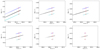 |
Fig. 3. Comparison of the distribution of sky positions after two days of propagation for asteroids with a different number of transits (From left to right and from top to bottom panels: 3, 4, 5, 6, 9, 12). The scale is the same for all cases. Black points represent the spreading of the orbits according to the old data model, blue points according to the new data model, turquoise points are validation points from OpenOrb, and the red cross is the correct position according to JPL Horizons. The points for the new data model and validation are shifted in declination for illustration purposes. For the three-transit case, the real spread along the line of variation does not fit on the same scale with other cases. The spread is in the order of 15° for the new data model and 60° for the old data model (Fig. 2 left). |
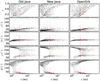 |
Fig. 4. Asteroid (425387) 2010 CZ61, with three transits. Comparison of Keplerian elements as a result of orbital inversion with different methods and codes. Left column, from top to bottom panels: Keplerian elements e, i, Ω, ω and M as a function of a for independent observations. Middle column: same elements, but for Java code with normal-point treatment. Right column: OpenOrb with normal-point treatment. The red cross denotes the correct position of the object. |
To further validate the approach, we performed a comparison between the known positions of the asteroids and predictions given by random-walk ranging that are based on a single-night batch of Gaia observations. We used 507 different asteroids with varying observational time-spans and numbers of transits. Our success rate (known position within the ephemeris distribution) was about 95%. The unsuccessful 5% corresponded to cases where the predicted ephemeris distribution was exceptionally compact when compared to the bulk of cases. After a two-day propagation, a typical offset of an unsuccessful prediction was of the order of 10′, a typical size of a side of a single CCD detector, and always along the line of variation. Therefore, even in these unsuccessful cases the recovery of an asteroid is still possible by extrapolating the search region along the line of variations.
We also performed a comparison on the effect of the number of sample orbits and their corresponding weights (Fig. 5). If not comparing single solutions but rather sums of solutions at given sky positions, 5000 orbits seem to give a statistically better prediction than the nominal 2000 orbits. The increase of the sample from 5000 orbits does not play a statistically significant role, as can be determined from the general shapes of the histograms in Fig. 5. As a rule, with the current configuration, the real solution corresponds to the upper third of the cumulative weight distribution.
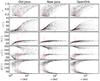 |
Fig. 5. Comparison of the sample orbit sizes and their respective weights between two codes (Java, top panel; OpenOrb; bottom panel) as a function of the right ascension of the sky positions of the propagated orbits for (420834) 2013 JX10, meaning an object with six transits. The sample sizes in each column from left to right are 2000, 5000, 20 000, and 50 000 orbits respectively. The correct position is designated by a vertical red dashed line in each case. |
We remind the reader that the velocity information of the transit is not used. As the quality of the velocity data been constantly improving, the addition of the velocity information to the normal-point treatment could be a potential improvement in the future.
Using the schematic in Fig. 1, we can interpret the differences between the old and the new models. In the old model, each observation was treated independently. The systematic error of each observation was reduced by a factor of  , where Nj is the number of observations in a single transit. This effectively shrank the systematic error bars, enhancing the curvature between the transits. The initial source for curvature is the apparent displacement of the asteroid position with regards to the true position in the short-term processing. This is a result of the variation of Gaia’s attitude (i.e. the difference between the black and the purple line in Fig. 1). We note that the curvature of the orbits is present for solutions that have close ranges.
In addition to the primary effect, two additional mechanisms are important to mention. First, the transits may have different amounts of observations between each other. The independent observation approach lead to assigning excessive weight to transits with higher amount of observations. This would affect the geometry of acceptable sample orbits. The solutions would bend towards the transits with more points. Second, the old model also permitted the inter-transit curvature of transits, which contributes even more to the bending of low-weight sample orbits.
The three mentioned separate effects lead to the bending of the orbits resulted in a large spread in i and Ω in the Keplerian phase space. The introduction of normal points effectively restored the level of the systematic error of an observation to a correct level. It also corrected for the different weighing of observations. Now all transits have the same weights, and the potentially erroneous inter-transit curvatures have been omitted by collapsing each transit into a single point.
It may appear that by collapsing transits into normal points valuable orientation and velocity information is lost for the observer. However, since the attitude of Gaia varies on a timescale similar to the duration of one transit, the inter-transit geometry is not a reliable source of information for the spatial orientation. Our analysis has shown that the correct assignment of weights is more important than the possibly lost information. We further note that the outlying close-solution orbits do not have exceptionally high weights compared to the bulk of sample orbits (Fig. 6). Furthermore, the area with formerly prevailing low-weight orbits is now completely depleted of solutions.
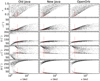 |
Fig. 6. Comparison of marginal pdfs in the proposed ranges of orbits for an asteroid with three transits in the old independent observation model (left panel), and the new normal-point model (right panel). |
In addition to the factors contributing to the bending of the orbits, there are two other minor mechanisms that generally deteriorate the ephemeris predictions. First, we note that for the short-term processing we are forced to keep the troublesome star mapper position in the fit as it is the only source of information for the across-scan direction, In the independent observation case this would result in the necessity to fit orbits to a number of outliers. Second, we suspect that an additional minor factor to the problem with the large search regions has at least in part been to the curvature of the line of variation. The aforementioned low-weight sample orbits, corresponding to close-range orbits with an offset of i and Ω values compared to the bulk of sample orbits, extend the customary line of variation to the point when it is curved on the sky. To cover the area including the curve, a large empty area is included in the search polygon. These low-weight sample orbits, which previously were the main contributor to the wide search area are now omitted. In the new calculations, all sample orbits are distributed along the line of variation. Therefore, the search area is shrunk to a single dimension.
4. Conclusions
We have improved orbital inversion for asteroids discovered by Gaia. The search area on the sky two days after the discovery is reduced by a factor of between three and ten when collapsing transits to normal points compared to the situation when all observations are treated separately. This means that assuming a typical field-of-view size of a telescope to be of the order of 10′×10′, the asteroid can now be recovered requiring only a few exposures along the line of variation. We emphasize that no improvement has been made for the orbital inversion method itself – the only difference is the treatment of the input data.
In this work we have shown that the proper treatment of random and systematic errors of asteroid observations can in some situations lead to significant improvements in their ephemeris predictions. In an era when automated surveys produce most asteroid discoveries it is essential to understand the error model and all the possible systematic error sources of each survey. In general, we show that treating a set of observations as a transit and using their normal point in orbit computation is a practical means to properly account for the contribution of systematic errors.
The predicted search areas for ground-based follow-up observers are now much better constrained than by using the previous input data model. We anticipate a significant increase in asteroid discoveries using the Gaia follow-up network predictions. With the approved two-year extension of Gaia, and a typical rate of a dozen new objects per night, in the order of 10 000 new SSOs can potentially be discovered in the years to come.
Acknowledgments
We are grateful to the anonymous referee, whose thoughtful and insightful comments improved the article. We would like to thank the staff of the DPCC, especially Eric Poujoulet, for their continuous support throughout the years. The authors are grateful for previous contributions by Tuomo Pieniluoma, Hanna Pentikäinen, and Dagmara Oszkiewicz. The work of GF has been supported by the Nordic Optical Telescope Scientific Association and the Emil Aaltonen foundation. MG is partly funded by the Academy of Finland (grant #299543). The work of AD’O and the Italian participation in DPAC has been supported by Agenzia Spaziale Italiana (ASI) through grants I/037/08/0, I/058/10/0, 2014-025-R.0, 2014-025-R.1.2015, and 2014-049-R.0/1/2 to INAF and contracts I/008/10/0 and 2013/030/I.0 to ALTEC S.p.A. and the Italian Istituto Nazionale di Astrofisica (INAF).
References
- Baer, J., Chesley, S. R., & Milani, A. 2011, Icarus, 212, 438 [NASA ADS] [CrossRef] [Google Scholar]
- Carpino, M., Milani, A., & Chesley, S. R. 2003, Icarus, 166, 248 [NASA ADS] [CrossRef] [Google Scholar]
- Carry, B. 2014, Gaia-FUN-SSO-3, 53 [Google Scholar]
- Chesley, S. R., Baer, J., & Monet, D. G. 2010, Icarus, 210, 158 [NASA ADS] [CrossRef] [Google Scholar]
- Farnocchia, D., Chesley, S., & Micheli, M. 2015b, Icarus, 258, 18 [NASA ADS] [CrossRef] [Google Scholar]
- Farnocchia, D., Chesley, S. R., Chamberlin, A. B., & Tholen, D. J. 2015a, Icarus, 245, 94 [NASA ADS] [CrossRef] [Google Scholar]
- Gaia Collaboration (Prusti, T., et al.) 2016, A&A, 595, A1 [NASA ADS] [CrossRef] [EDP Sciences] [Google Scholar]
- Gaia Collaboration (Mignard, F., et al.) 2018a, A&A, 616, A14 [NASA ADS] [CrossRef] [EDP Sciences] [Google Scholar]
- Gaia Collaboration (Spoto, F., et al.) 2018b, A&A, 616, A13 [NASA ADS] [CrossRef] [EDP Sciences] [Google Scholar]
- Granvik, M., Morbidelli, A., Jedicke, R., et al. 2018, Icarus, 312, 181 [Google Scholar]
- Granvik, M., Virtanen, J., Oszkiewicz, D. A., & Muinonen, K. 2009, Meteorit. Planet. Sci., 44, 1853 [NASA ADS] [CrossRef] [Google Scholar]
- Jeffreys, H. 1946, Proc. R Stat. Soc. London, Ser. A, 186, 453 [Google Scholar]
- Jordi, C., Gebran, M., Carrasco, J. M., et al. 2010, A&A, 523, A48 [NASA ADS] [CrossRef] [EDP Sciences] [Google Scholar]
- Mahlke, M., Bouy, H., Altieri, B., et al. 2018, A&A, 610, A21 [NASA ADS] [CrossRef] [EDP Sciences] [Google Scholar]
- Mignard, F., Cellino, A., Muinonen, K., et al. 2007, Earth Moon Planets, 101, 97 [Google Scholar]
- Muinonen, K., & Bowell, E. 1993, Icarus, 104, 255 [NASA ADS] [CrossRef] [Google Scholar]
- Muinonen, K., & Lumme, K. 2015, A&A, 584, A23 [NASA ADS] [CrossRef] [EDP Sciences] [Google Scholar]
- Muinonen, K., Virtanen, J., & Bowell, E. 2001, Celest. Mech. Dyn. Astron., 81, 93 [NASA ADS] [CrossRef] [Google Scholar]
- Muinonen, K., Granvik, M., Oszkiewicz, D., Pieniluoma, T., & Pentikäinen, H. 2012, Planet. Space Sci., 73, 15 [Google Scholar]
- Muinonen, K., Fedorets, G., Pentikäinen, H., et al. 2016, Planet. Space Sci., 123, 95 [NASA ADS] [CrossRef] [Google Scholar]
- O’Hagan, A., & Forster, J. 2004, Kendall’s Advanced Theory of Statistics, 2nd edn. (Arnold), 2B, Bayesian Inference [Google Scholar]
- Oszkiewicz, D., Muinonen, K., Virtanen, J., & Granvik, M. 2009, Meteor. Planet. Sci., 44, 1897 [Google Scholar]
- Oszkiewicz, D., Muinonen, K., Virtanen, J., Granvik, M., & Bowell, E. 2012, Planet. Space Sci., 73, 30 [NASA ADS] [CrossRef] [Google Scholar]
- Ribeiro, A. O., Roig, F., De Prá, M. N., Carvano, J. M., & DeSouza, S. R. 2016, MNRAS, 458, 4471 [NASA ADS] [CrossRef] [Google Scholar]
- Siltala, L., & Granvik, M. 2017, Icarus, 297, 149 [NASA ADS] [CrossRef] [Google Scholar]
- Tanga, P., Mignard, F., Dell’Oro, A., et al. 2016, Planet. Space Sci., 123, 87 [NASA ADS] [CrossRef] [Google Scholar]
- Thuillot, W., Carry, B., Berthier, J., et al. 2014, in SF2A-2014: Proceedings of the Annual meeting of the French Society of Astronomy and Astrophysics, eds. J. Ballet, F. Martins, F. Bournaud, R. Monier, & C. Reylé, 445 [Google Scholar]
- Vereš, P., Farnocchia, D., Chesley, S. R., & Chamberlin, A. B. 2017, Icarus, 296, 139 [NASA ADS] [CrossRef] [Google Scholar]
- Virtanen, J., & Muinonen, K. 2006, Icarus, 184, 289 [NASA ADS] [CrossRef] [Google Scholar]
- Virtanen, J., Muinonen, K., & Bowell, E. 2001, Icarus, 154, 412 [NASA ADS] [CrossRef] [Google Scholar]
Appendix A: Additional figures
All Tables
Values of mean ranges and their standard deviations used as initial guesses in the Gaia orbital inversion software.
All Figures
|
Fig. 1. Along-scan position of an asteroid as a function of time in Gaia short-term processing. The purple line depicts the true position of the asteroid, and the black line depicts the position suffering systematically from the uncertainties in the Gaia attitude model. Blue bars describe observations and their random errors grouped in transits, red points are normal points, and red lines are systematic errors. The treatment of the across-scan position is analogous. |
| In the text | |
|
Fig. 2. Left panel: spread on the sky after two days of propagation for an object with three transits. Black points represent the spreading of the orbits according to the old data model, blue points according to the new data model, turquoise points are validation points from OpenOrb, and the red cross is the correct position according to JPL Horizons. The points for the new data model and validation are shifted in declination for illustration purposes. Right panel: magnification of spread across the line of variation. The width of the spread is around 20″. |
| In the text | |
|
Fig. 3. Comparison of the distribution of sky positions after two days of propagation for asteroids with a different number of transits (From left to right and from top to bottom panels: 3, 4, 5, 6, 9, 12). The scale is the same for all cases. Black points represent the spreading of the orbits according to the old data model, blue points according to the new data model, turquoise points are validation points from OpenOrb, and the red cross is the correct position according to JPL Horizons. The points for the new data model and validation are shifted in declination for illustration purposes. For the three-transit case, the real spread along the line of variation does not fit on the same scale with other cases. The spread is in the order of 15° for the new data model and 60° for the old data model (Fig. 2 left). |
| In the text | |
|
Fig. 4. Asteroid (425387) 2010 CZ61, with three transits. Comparison of Keplerian elements as a result of orbital inversion with different methods and codes. Left column, from top to bottom panels: Keplerian elements e, i, Ω, ω and M as a function of a for independent observations. Middle column: same elements, but for Java code with normal-point treatment. Right column: OpenOrb with normal-point treatment. The red cross denotes the correct position of the object. |
| In the text | |
|
Fig. 5. Comparison of the sample orbit sizes and their respective weights between two codes (Java, top panel; OpenOrb; bottom panel) as a function of the right ascension of the sky positions of the propagated orbits for (420834) 2013 JX10, meaning an object with six transits. The sample sizes in each column from left to right are 2000, 5000, 20 000, and 50 000 orbits respectively. The correct position is designated by a vertical red dashed line in each case. |
| In the text | |
|
Fig. 6. Comparison of marginal pdfs in the proposed ranges of orbits for an asteroid with three transits in the old independent observation model (left panel), and the new normal-point model (right panel). |
| In the text | |
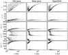 |
Fig. A.1. Same as Fig. 4 but for asteroid (414265) 2008 GC113, with four transits. |
| In the text | |
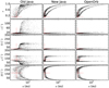 |
Fig. A.2. Same as Fig. 4 but for asteroid (462915) 2011 AC21 with five transits. |
| In the text | |
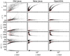 |
Fig. A.3. Same as Fig. 4 but for asteroid (420834) 2013 JX10 with six transits. |
| In the text | |
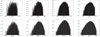 |
Fig. A.4. Same as Fig. 4 but for asteroid (150016) 2005 UB353 with nine transits. |
| In the text | |
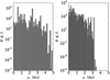 |
Fig. A.5. Same as Fig. 4 but for asteroid (274721) 2008 UH155 with twelve transits. |
| In the text | |
Current usage metrics show cumulative count of Article Views (full-text article views including HTML views, PDF and ePub downloads, according to the available data) and Abstracts Views on Vision4Press platform.
Data correspond to usage on the plateform after 2015. The current usage metrics is available 48-96 hours after online publication and is updated daily on week days.
Initial download of the metrics may take a while.