Erratum for: A&A, 580, A124 (2015), https://doi.org/10.1051/0004-6361/201526104

1. Introduction

A missing normalization coefficient in Eqs. (11) and (12) of de Avillez & Breitschwerdt (2015) affected the results shown in Figs. 3 and 4 and discussed in Sect. 3 of that earlier publication. Here, we present the corrected version of the equations and the corresponding results discussed in Sect. 3 and shown in Figs. 3 and 4 of that paper. In addition we provide supplementary material in the form of tables covering a larger parameter space than the one previously used. These tables are available at the CDS.

2. Temperature-averaged and total Gaunt factor

During the interaction of an electron with the Coulomb field of an ion of ionic state z and atomic number Z the amount of free-free energy emitted per unit time and unit volume is given by

$$\begin{array}{c}\hfill \frac{d{P}_{{}_{\mathrm{ff}}}}{\mathit{du}}=\frac{8{\pi }^2}{h{c}^3}{\left(\frac{2}{3m_e}\right)}^{3/2}{e}^6{z}^2{n}_e{n}_{{}_{Z,z}}{k}_{B}T{N}_e⟨g_{\mathit{ff}}({\gamma }^2,u)⟩,\end{array}$$(1)

with z denoting the ionic state of an ion with atomic number Z and number density n_{Z, z}, n_e is the electron number density, h is the Planck constant, c is the speed of light, e is the electron charge in Coulombs, m_e is the electron mass, k_B is the Boltzmann constant, T is the temperature, and ⟨g_ff(γ², u)⟩ is the temperature averaged Gaunt factor given by (see, e.g., de Avillez & Breitschwerdt 2017)

$$\begin{array}{l}\begin{array}{l}\langle g_{ff}({\gamma }^2,u)\rangle =\frac{{(k_{B}T)}^{1/2}}{N_e}\hfill \\ \times {\displaystyle {\int }_0^{+\infty }\frac{1}{{(y+u)}^{1/2}}}f[(y+u)k_{B}T]g_{ff}\left({ϵ}_i=\frac{y+u}{{\gamma }^2},{ϵ}_f=\frac{y}{{\gamma }^2}\right)dy\hfill \end{array}\hfill \end{array}$$(2)

where f is the electron distribution function, u = hν/k_BT (ν is the frequency of the emitted photon), γ² = z²Ry/k_BT (Ry is the Rydberg constant), and N_e is a normalization coefficient defined such ⟨g_{f f}(γ², u)⟩ = 1 when g_{f f}(γ², u)=1. For the κ and Maxwell-Boltzmann (MB) electron distribution functions N_e is given by

$$\begin{array}{c}\hfill N_e=\{\begin{array}{ccc}{\displaystyle \frac{2}{\sqrt{\pi k_{B}T}}{\int }_0^{+\infty }G(y+u;\kappa )dy}\hfill & \mathrm{if}\hfill & \kappa >3/2\hfill \\ \hfill & \hfill & \\ {\displaystyle \frac{2e^{-u}}{\sqrt{\pi k_{B}T}}}\hfill & \mathrm{if}\hfill & \mathit{MB},\hfill \end{array}\end{array}$$(3)

with

$$\begin{array}{c}\hfill G(x;\kappa )=\frac{A_{\kappa }}{{\displaystyle {[1+\frac{x}{\kappa -3/2}]}^{\kappa +1}}},\end{array}$$(4)

and

$$\begin{array}{c}\hfill {\displaystyle {\int }_0^{+\infty }G(y+u;\kappa )dy=A_{\kappa }\frac{\kappa -3/2}{\kappa }{(1+\frac{u}{\kappa -3/2})}^{-\kappa },}\end{array}$$(5)

which becomes e^−u when κ → ∞ (Fig. 1). In these expressions

$$\begin{array}{c}\hfill A_{\kappa }=\frac{\mathrm{\Gamma }(\kappa +1)}{\mathrm{\Gamma }(\kappa -1/2){(\kappa -3/2)}^{3/2}}\text{and}\kappa >3/2.\end{array}$$(6)

Therefore, Eq. (11) in de Avillez & Breitschwerdt (2015) must be rewritten as

$$\begin{array}{l}\frac{d{P}_{\text{ff}}}{du}=C_{\text{ff}}{z}^2{n}_e{n}_{Z,z}{T}^{1/2}\hfill \\ \{\begin{array}{lll}\frac{1}{{\displaystyle {\int }_0^{+\infty }G(y+u;k)dy}}{\displaystyle {\int }_0^{+\infty }{g}_{\text{ff}}({\gamma }^2,u)G(y+u;\kappa )dy}\hfill & \text{if}\hfill & \kappa >3/2\hfill \\ e^{-u}{\displaystyle {\int }_0^{+\infty }{g}_{\text{ff}}({\gamma }^2,u)e^{-y}dy}\hfill & \text{if}\hfill & \text{MB.}\hfill \end{array}\hfill \end{array}$$(7)

where

$$\begin{array}{c}\hfill {\displaystyle C_{{}_{\mathrm{ff}}}=16{\left(\frac{2\pi }{3m_{{}_e}}\right)}^{3/2}\frac{e^6{k}_B^{1/2}}{h{c}^3}=1.4256\times {10}^{-27}\text{erg}\text{cm}{3}^{}{\text{s}}^{-1}{\text{K}}^{-1/2}.}\end{array}$$

The total free-free power associated with an ion (Z, z) given by

$$\begin{array}{c}\hfill P_{{}_{\mathrm{ff}}}(T)=C_{{}_{\mathrm{ff}}}{z}^2{n}_e{n}_{{}_{Z,z}}{T}^{1/2}{\displaystyle {\int }_0^{+\infty }⟨g_{{}_{\mathrm{ff}}}({\gamma }^2,u)⟩f(u)du}\end{array}$$(8)

with

$$\begin{array}{c}\hfill f(u)=\{\begin{array}{ccc}{\displaystyle {\int }_0^{+\infty }G(y+u;\kappa )dy}\hfill & \mathrm{if}\hfill & \kappa >3/2\hfill \\ \hfill & \hfill & \\ {\displaystyle e^{-u}}\hfill & \mathrm{if}\hfill & \text{MB}.\hfill \end{array}\end{array}$$(9)

The integral in the RHS of (8) is the total free-free Gaunt factor. When κ → ∞ the Integral in (9) tends to e^−u and total Gaunt factor for the MB distribution of electrons as defined by Karzas & Latter (1961) is recovered

$$\begin{array}{c}\hfill g_{\mathit{ff}}(T)={\displaystyle {\int }_0^{+\infty }⟨g_{\mathit{ff}}({\gamma }^2,u)⟩e^{-u}du.}\end{array}$$(10)

The top panel of Fig. 2 and the panels in Fig. 3 display the variation with γ² of the temperature-averaged Gaunt factor, ⟨g_{f f}(γ², u)⟩, for different values of u ∈ [10⁻⁴, 10⁴] for the MB and κ = 2, ...,1200 distributions. The bottom panel of Fig. 2 highlights in a magnified image of the region γ² ∈ [10⁻², 10⁶] the distribution with γ² of ⟨g_{f f}(γ², u)⟩ for different values of u.

It is clear that as κ increases the temperature-averaged κ distributed Gaunt factors approach those calculated with the MB distribution. However, the speed (with κ variation) of this approach depends on the values of u. For u < 10 this approach is faster than for u ≥ 10 (compare top panel of Fig. 2 and the two panels in Fig. 3). For values as high as κ = 1200 there is still no overlap between the κ and Maxwellian values of ⟨g_{f f}(γ², u)⟩ for u > 10² and γ² < 10 (Fig. 3). This is a consequence of the slow approach to e^−u of the integral ${\int }_0^{+\infty }G(\mathit{y}+u;\kappa )dy$ for u ≥ 10 in comparison to u < 10 (Fig. 1).

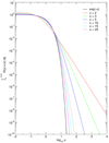Fig. 1. Variation of Integral (5) with κ as function of u. The solid black line represents e−u which is overlapped by the integral as κ → ∞.

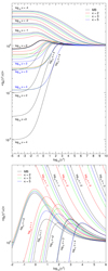Fig. 2. Temperature-averaged Gaunt factors calculated for κ = 2, 3, 5 and MB (black line in both panels) distributions of electrons for the range 10−5 ≤ γ2 ≤ 1010 (top panel) and a magnification of the region γ2 ∈ [10−2, 106] and ⟨gf f(γ2, u)⟩ ∈ [0.9, 1.5] (bottom panel).

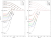Fig. 3. Temperature-averaged Gaunt factors calculated for κ = 10, 15, 25, and 50 (left panel), 100, 500, 1000, and 1200 (right panel) and MB (black line in both panels) distributions of electrons for the range 10−5 ≤ γ2 ≤ 1010. We note the slow approach ⟨gf f(γ2, u)⟩ to the Maxwellian values for u > 10 and γ2 < 10 for large values of the κ parameter.

Figure 4 displays the total free-free Gaunt factor, ⟨g_{f f}(γ²)⟩, calculated for the MB and κ = 2, 3, 5, 10, 15, and 25 distributions. For larger κ the ⟨g_{f f}(γ²)⟩ almost overlap with the Maxwellian value as shown in the magnification of the regions ⟨g_{f f}(γ²)⟩ ∈ [ − 1.0, 0.8] and ⟨g_{f f}(γ²)⟩ ∈ [1.38, 1.45] (top panel of Fig. 5), and ⟨g_{f f}(γ²)⟩ ∈ [6, 10] and ⟨g_{f f}(γ²)⟩ ∈ [0.995, 1.005] (bottom panel of same Figure). It turns out that even for κ parameters as high as 1000 there is still a slight difference between ⟨g_{f f}(γ²)⟩ calculated for the κ and MB distributions.

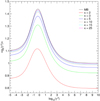Fig. 4. Total free-free Gaunt factor calculated for κ(2, 3, 5, 10, 15, and 25) and MB distributions.

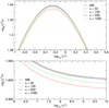Fig. 5. Magnification of the total free-free Gaunt factor in two regions in γ2 and in the ⟨gf f(γ2)⟩ profile shown in Fig. 4 but for κ = 50, 100, 500, and 1000. The solid black line refers to the Maxwellian value.

3. Tables

Supplementary material is available at the CDS with a set of tables referring to the temperature-averaged Gaunt factor versus γ² and different u, and a table for the total Gaunt factor versus γ² for results obtained with the κ = 2, 3, 5, 10, 15, 25, 50, 100, and 500 and MB electron distributions. The parameter space comprises γ² ∈ [10⁻⁵, 10¹⁰] and u ∈ [10⁻¹², 10¹¹].

Acknowledgments

This research was supported by the project Enabling Green E-science for the SKA Research Infrastructure (ENGAGE SKA), reference POCI-01-0145-FEDER-022217, funded by COMPETE 2020 & FCT, Portugal.

References

© ESO 2018

All Figures

	Fig. 1. Variation of Integral (5) with κ as function of u. The solid black line represents e−u which is overlapped by the integral as κ → ∞.
In the text

	Fig. 2. Temperature-averaged Gaunt factors calculated for κ = 2, 3, 5 and MB (black line in both panels) distributions of electrons for the range 10−5 ≤ γ2 ≤ 1010 (top panel) and a magnification of the region γ2 ∈ [10−2, 106] and ⟨gf f(γ2, u)⟩ ∈ [0.9, 1.5] (bottom panel).
In the text

	Fig. 3. Temperature-averaged Gaunt factors calculated for κ = 10, 15, 25, and 50 (left panel), 100, 500, 1000, and 1200 (right panel) and MB (black line in both panels) distributions of electrons for the range 10−5 ≤ γ2 ≤ 1010. We note the slow approach ⟨gf f(γ2, u)⟩ to the Maxwellian values for u > 10 and γ2 < 10 for large values of the κ parameter.
In the text

	Fig. 4. Total free-free Gaunt factor calculated for κ(2, 3, 5, 10, 15, and 25) and MB distributions.
In the text

	Fig. 5. Magnification of the total free-free Gaunt factor in two regions in γ2 and in the ⟨gf f(γ2)⟩ profile shown in Fig. 4 but for κ = 50, 100, 500, and 1000. The solid black line refers to the Maxwellian value.
In the text

References

- de Avillez, M. A., & Breitschwerdt, D. 2015, A&A, 580, A124 [NASA ADS] [CrossRef] [EDP Sciences] [Google Scholar]
- de Avillez, M. A. & Breitschwerdt, D. 2017, ApJS, 232, 12 [NASA ADS] [CrossRef] [Google Scholar]
- Karzas, W. J. & Latter, R. 1961, ApJS, 6, 167 [NASA ADS] [CrossRef] [Google Scholar]