| Issue |
A&A
Volume 619, November 2018
|
|
|---|---|---|
| Article Number | A50 | |
| Number of page(s) | 10 | |
| Section | Galactic structure, stellar clusters and populations | |
| DOI | https://doi.org/10.1051/0004-6361/201833755 | |
| Published online | 07 November 2018 | |
The spiral potential of the Milky Way⋆,⋆⋆
1 European Southern Observatory, Karl-Schwarzschild-Str. 2, 85748 Garching, Germany
e-mail: giovanni.carraro@unipd.it
2 Dipartimento di Fisica e Astronomia, Universita’ di Padova, Vicolo Osservatorio 3, 35122 Padua, Italy
e-mail: pgrosbol@eso.org
Received:
2
July
2018
Accepted:
20
August
2018
Context. The location of young sources in the Galaxy suggests a four-armed spiral structure, whereas tangential points of spiral arms observed in the integrated light at infrared and radio wavelengths indicate that only two arms are massive.
Aims. Variable extinction in the Galactic plane and high light-to-mass ratios of young sources make it difficult to judge the total mass associated with the arms outlined by such tracers. The current objective is to estimate the mass associated with the Sagittarius arm by means of the kinematics of the stars across it.
Methods. Spectra of 1726 candidate B- and A-type stars within 3◦ of the Galactic center (GC) were obtained with the FLAMES instrument at the VLT with a resolution of ≈6000 in the spectral range of 396–457 nm. Radial velocities were derived by least-squares fits of the spectra to synthetic ones. The final sample was limited to 1507 stars with either Gaia DR2 parallaxes or main-sequence B-type stars having reliable spectroscopic distances.
Results. The solar peculiar motion in the direction of the GC relative to the local standard of rest (LSR) was estimated to U⊙ = 10.7 ± 1.3kms−1. The variation in the median radial velocity relative to the LSR as a function of distance from the sun shows a gradual increase from slightly negative values near the sun to almost 5 km s−1 at a distance of around 4 kpc. A sinusoidal function with an amplitude of 3.4 ± 1.3kms−1 and a maximum at 4.0 ± 0.6 kpc inside the sun is the best fit to the data. A positive median radial velocity relative to the LSR around 1.8 kpc, the expected distance to the Sagittarius arm, can be excluded at a 99% level of confidence. A marginal peak detected at this distance may be associated with stellar streams in the star-forming regions, but it is too narrow to be associated with a major arm feature.
Conclusions. A comparison with test-particle simulations in a fixed galactic potential with an imposed spiral pattern shows the best agreement with a two-armed spiral potential having the Scutum–Crux arm as the next major inner arm. A relative radial forcing dFr ≈ 1.5% and a pattern speed in the range of 20–30 km s−1 kpc−1 yield the best fit. The lack of a positive velocity perturbation in the region around the Sagittarius arm excludes it from being a major arm. Thus, the main spiral potential of the Galaxy is two-armed, while the Sagittarius arm is an inter-arm feature with only a small mass perturbation associated with it.
Key words: Galaxy: disk / Galaxy: structure / Galaxy: kinematics and dynamics / stars: early-type / techniques: spectroscopic
Based on observations collected at the European Southern Observatory, Chile (ESO programme 097.B-00245, 099.B-0697).
The catalog of radial velocities is only available at the CDS via anonymous ftp to cdsarc.u-strasbg.fr (130.79.128.5) or via http://cdsarc.u-strasbg.fr/vizbin/qcat?J/A+A/619/A50
© ESO 2018
1. Introduction
The first evidence of spiral structure in the Milky Way was presented in the 1950s; it was obtained from optical observations of early-type stars first, and from H I surveys shortly thereafter (see Gingerich 1985; Carraro 2015). Both techniques have several well-known disadvantages, yet they were extensively used in the past, and nowadays there are even claims that the issue of the spiral structure of our Galaxy has been solved (Hou & Han 2014). While optical observations are limited by the extinction problem, H I surveys suffer from the inability to derive reliable distances from radial velocity, and from the fact that H I is almost evenly distributed across the Galactic disk (Liszt 1985). Traditionally, long-wavelength observations depict a two-armed Milky Way, while optical observations favor a four-armed Milky Way. Recent, extensive mapping of young objects (e.g., OB-associations, H II-regions, and young clusters) were presented by Russeil (2003) and revealed indications of a four-armed spiral structure. On the contrary, the tangent associated with the Sagittarius arm observed in near-infrared bands shows no significant increase in integrated intensity (Drimmel 2000). This suggests that little mass is associated with this arm, as near-infrared surface brightness is well correlated to stellar mass density, and that the Galaxy has a two-armed structure with Scutum–Crux as the next major arm inside the sun.
These two scenarios need not contradict each other as secondary shocks in the gas can be produced by a two-armed spiral perturbation (Yáñez et al. 2008) leading to increased star formation between the major arms. A four-armed gas spiral may also be excited by the Galactic bar (Englmaier & Gerhard 1999, 2006). For external spiral galaxies, the appearance in the near-infrared is much smoother with weaker inter-arm features than on visual images (Block et al. 1994; Grosbøl & Patsis 1998; Eskridge et al. 2002) as the former emphasizes the cold stellar disk population and therefore the surface density of the disks.
The structure of star-forming regions is important, but the shape of the spiral potential is essential for the dynamics of the Galaxy. The high light-to-mass ratio of young objects makes it very difficult to deduce the mass distribution from them. A more direct method of estimating the mass variation associated with nearby spiral arms is star counts of a well-defined stellar population as a function of the distance from the sun. This was done for the Perseus arm in the anti-center direction using early-type stars for which individual distances can be determined (Monguió et al. 2015). For the Sagittarius arm, the high and patchy extinction toward the Galactic center (GC) makes it impossible to conduct a reliable star count. The potential perturbation can also be evaluated by measuring the velocity field of a relaxed stellar population across arms. One concern for very young stars is that they may not be fully dynamically relaxed and still be biased by their initial velocity. An unbiased, random sample of velocities of a well-defined stellar population allows an estimate of the perturbation independent of the high, patchy extinction toward the GC assuming that they are uncorrelated.
The current paper studies the variations in radial velocities as a function of distance for a sample of late B- and A-stars toward the GC with the aim of determining a velocity perturbation associated with the Sagittarius arm. The sample is described in Sect. 2 where the observations are detailed as well. The next section presents the reduction of the data and the derivation of individual radial velocities and distances for the sources. Possible models for the spiral potential in the Milky Way is discussed in Sect. 4, while the conclusions are given in Sect. 5.
2. Targets and observations
Velocity variations across arms in grand-design spirals measured in H I are on the order of 10 km s−1 (see, e.g., Visser 1980a,b for M 81). This sets an upper limit for the expected velocity change of a stellar population since its response to a potential perturbation decreases with higher velocity dispersion (Lin et al. 1969; Shu 1970; Mark 1976). A velocity variation with this amplitude is easier to detect in a population with an intrinsic low-velocity dispersion, such as stars with ages of less than 2 Gyr (Yu & Liu 2018). The population should also be old enough to be dynamically relaxed in the Galactic potential that required several encounters with the spiral perturbations, i.e., at least 300 Myr. Thus, late B- and A-stars are the best populations for the study of the effects of the spiral potential on the stellar velocity field. Selecting targets towards the GC, we can avoid any significant influence of the Galactic differential rotation on the measured velocity variation, which outweighs other issues like crowding and high extinction.
The velocity dispersion of B- and A-stars in the solar neighborhood is around 20 km s−1 (Yu & Liu 2018) which indicates that a sample of several hundred sources is required for a 5σ detection of an average velocity perturbation of 5–10 km s−1. A critical point for distinguishing between a two- or four-armed spiral potential in the Milky Way is the velocity perturbation associated with the Sagittarius arm, which is located 1.8 kpc inside the solar radius in the direction toward the GC (Reid et al. 2014; Wu et al. 2014) corresponding to a distance modulus of 11m. A sample of early-type stars with B < 15m should include sources beyond the Sagittarius arm, even with visual extinctions in the range of 5m.
Due to the high extinction toward the GC, it is difficult to select B- and A-stars based on their colors since nearby late-type stars have colors similar to highly reddened early-type stars. Therefore, the prime targets were taken from the catalog of early-type stars by Grosbøl (2016) based on objective prism observations. The positional errors of this catalog (i.e., σα ≈ 1″, σδ ≈ 6″) did not allow a direct cross-match with other catalogs, due to the high stellar density toward the GC. Selecting sources from VVV (Saito et al. 2012) with the reddening corrected color index Q = (H − K) − 0.563 × (J − H) (Indebetouw et al. 2005) matching early-type stars (i.e. −0ṃ1 < Q < 0ṃ1) and Ks < 14m, the density was reduced enough to secure a unique matching of the targets.
The most efficient facility for observing spectra of the candidates was the FLAMES instrument (Pasquini et al. 2002) at the ESO/VLT, which in its GIRAFFE/MEDUSA mode offers 130 fibers with a 1″̣2 diameter in a circular field with a radius of 15′. A total of 15 fields were defined selecting the area with the highest density of prime targets, yielding 17–54 sources per field. Additional candidates were selected for the remaining fibers by picking VVV sources with reddening corrected colors corresponding to early-type stars and estimated blue magnitudes B < 15m.
Five FLAMES/GIRAF fields were observed in 2016 (i.e., ESO P97) for which VVV positions were used to center the fibers, leading to some errors due to the differences in epoch. The observations of the ten remaining fields were done in 2017 for which Gaia DR1 positions (Gaia Collaboration 2016b, 2016a; Arenou et al. 2017) were adopted, which significantly improved the centering and thereby their signal-to-noise ratio (S/N) for the same apparent magnitude. The LR2 grating was used with a spectral resolution R = 6000 in the range of λ = 396−456 nm.
The observations are summarized in Table 1, which lists the 15 fields with their Galactic coordinates (lII,bII) and the Modified Julian Date (MJD) of their mean exposure. The total number of fibers allocated, nt, is also given including the fibers used for prime targets, np. For each field, 7–16 fibers were allocated to sky positions with no stars visible on the Digital Sky Survey 2 images using Aladin (Bonnarel et al. 2000). Four exposures of 660 s duration (in P97 only 600 s) were made of each field to allow for removal of cosmic ray events and extend the dynamic range. The observations were conducted in service mode and yielded a total of 1726 spectra of which 1505 had a S/N higher than 10. The seeing was in the range of 0.8–1.4″, while the sky conditions were specified to allow for thin clouds. A cross-matching based on positions gave 1635 sources with Ks-magnitudes in the VVV catalog, while 1608 were listed in the Gaia DR2 catalog with parallaxes (Gaia Collaboration 2018a).
Summary of VLT/FLAMES observations.
3. Radial velocities and distances
The basic reductions including flat-fielding and wavelength calibration were done via the standard ESO pipeline (Giraf/2.16.1) as processed by the observatory. For each field, the four exposures were averaged after outliers (e.g., cosmic ray events) were removed with a median filter. The spectra were normalized to the continuum estimated by fitting a low-order polynomial to the median values of sections with a few spectrum lines. Radial velocities were derived by matching the spectra with model grids of synthetic spectra performing both a cross-correlation and least-squares fitting. The synthetic spectra were smoothed with a Gaussian filter and rebinned to match the observed spectra. In addition, a high-pass filter was applied to both synthetic and observed spectra to reduce biases due to errors in the normalization. The least-squares fits were preferred as they are less biased by the Balmer lines than the cross-correlation estimates. The spectral range for the comparison was limited to 399–454 nm as the spectra did not fully include the H∊ line. In addition to the fit to this range, five subsections of the spectra were used including two centered on the Balmer lines and three in the regions in between. This allowed us to verify whether the velocities estimated from the Balmer lines and metal lines were consistent. The weighted mean of these five estimates was adopted as the radial velocity after which the barycentric correction was added. Several grids were applied, such as the POLLUX (Palacios et al. 2010), UVBLUE (Rodríguez-Merino et al. 2005), and PHOENIX databases (Husser et al. 2013). Since no significant differences between these grids were found, the UVBLUE database was used as it provides a finer mesh. Due to the metallicity gradient in the Galactic disk, it is expected that stars inside the solar radius have higher metallicities than the sun. Grids with [M/H] = 0.3 were adopted since models with higher metallicities gave worse fits. In addition to radial velocity, effective temperature Teff and surface gravity g for the individual stars were estimated through the least-squares fitting. The distribution of sources is shown in Fig. 1 as a function of their effective temperature Teff. The surface gravity could only be determined reliably for stars with log(Teff) > 4.0 for which Balmer and He I lines are sensitive to g. Typical errors for the radial velocities are 3 km s−1 for stars with log(Teff) > 3.9, while for cooler stars they increase to around 5km s−1.
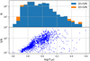 |
Fig. 1. Distribution of sources as a function of their effective temperature Teff. The upper diagram gives the histogram of sources while the lower one shows the signal-to-noise ratio (S/N) both in logarithmic scale. |
Since many sources were selected based on their near-infrared colors, the sample includes more than 100 late-type stars (see Fig. 1) with Teff in the range in which the Gaia DR2 database (Gaia Collaboration 2018a) provides radial velocities. A total of 63 common sources with both Gaia and FLAMES radial velocities were identified. A linear regression gave  . The velocities measured were corrected for this offset by adding 2.5 km s−1.
Absolute magnitudes and intrinsic colors for the sources were obtained from the Padova evolutionary tracks (Bressan et al. 2012; Marigo et al. 2017) using the Teff and g values derived. Models with metallicity Z = 0.03 were adopted. The VISTA filters were used as the best proxy for the VVV color system. The color index (Z − H) was used to obtain the largest wavelength difference of the bands while omitting Ks, which may be affected by Brγ emission. Extinctions were derived from the intrinsic colors using an extinction law λ−β with β = 1.517 (Schlafly & Finkbeiner 2011) yielding the excess E(Z − H) = 0.302 A(V) = 2.364 A(Ks). Distances were calculated from the Ks-band colors applying the A(Ks) extinction correction when positive. The 1″ aperture VVV magnitudes were used in order to reduce the contamination from nearby stars in the very crowded fields.
Although only five sources show clear double line profiles in their Balmer lines, we must assume that a large fraction of the sources are multiple-star systems (Duchêne & Kraus 2013). In the worst-case scenario where all systems are binaries with equal luminosity, the spectroscopic distances should be increased by 40%. In a more realistic case, the correct distances would be 10– 20% longer and potential features in the velocities as a function of distance would be smoothed.
The near-infrared extinction A(Ks) as a function of distance from the sun, d, is shown in Fig. 3 where the median values in radial bins of 0.5 kpc are also indicated with corresponding error bars. The extinction displays a large scatter, but its median increases to a distance of nearly 1.4 kpc, after which it remains nearly constant. The flat behavior at larger distances is likely a selection effect as only sources with a low extinction will appear in the current magnitude-limited sample. A second rise in the extinction at a distance of 4.3 kpc is suggested. Both of these step-wise increases may be caused by the star-forming regions in the arms.
Of the 1608 sources with Gaia parallaxes, 469 stars have reliable log(g) estimates (i.e., log(Teff) > 4.0) and therefore spectroscopic distances. These distances are, in general, consistent with the parallaxes (see Fig. 2) except for two groups of stars. One group with around 60 stars has significantly shorter distances than given by the Gaia parallaxes, likely caused by multiple-star systems. This group has on average larger errors which may be due to their multiplicity. Another set of almost 80 stars has much larger spectroscopic distances as the spectral fits suggested that they were giants, i.e., log(g) < 3.5. Distances calculated from the Gaia DR2 parallaxes were adopted for 1484 sources with parallaxes larger than 3.0 times their error. The error distribution of distances is skewed to longer distances assuming Gaussian errors for the parallaxes. This effect was estimated using a Monte Carlo simulation of errors which showed that the shift is less than 0.5 kpc for distances up to 3 kpc. Thus, in the worse-case scenario where all parallaxes have 33% relative errors, the distances will be underestimated by around 20%. In addition, spectroscopic distance were used for 45 main-sequence stars with log(Teff) > 4.0 and S/N > 10 yielding a total sample of 1529 sources. It should be noted that distances are correlated with the Teff estimates and therefore ages since the sample is magnitude limited.
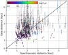 |
Fig. 2. Distances from Gaia DR2 parallaxes as a function of the distances determined from the spectra observed for stars with 4.0 < log(Teff). Stars with log(g) < 3.5 are indicated by crosses. |
The lower panel of Fig. 3 displays the barycentric radial velocities together with their median  as a function of their distance d, while the numeric values are listed in Table 2. The velocity distribution contains 12 outliers with velocities
  , all with positive residuals while 8 had S/N < 10. They were omitted as they are unlikely to be associated with the young stellar disk population. This left 1517 stars with a median velocity of −13.2 ± 0.7km s−1 and a dispersion of 26.8 km s−1. The former is consistent with the peculiar motion of the sun relative to LSR U⊙ = 11.1 ± 0.7km s−1 (Schönrich et al. 2010). The dispersion is slightly higher than that measured for the local young population (Yu & Liu 2018) due to the variation in the average as a function of distance and multiple-star systems. The mean radial velocities corrected to the LSR are negative close to the sun and then increase to positive values with a maximum at around 4 kpc. The peak-to-peak velocity variation is almost 8 km s−1.
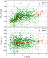 |
Fig. 3. Near-infrared extinction A(Ks) and barycentric radial velocity Vr as a function of distance d from the sun. |
List of the number of sources N, mean velocity  , standard deviation σ(Vr), and median velocity
  in km s−1 including their errors in distance bins centered on d (kpc).
4. Discussion
The statistics of the velocities were computed in 0.5 kpc radial bins in the range of 0.5–5.0 kpc containing a total of 1507 stars; they are listed in Table 2, where the two last bins were joined due to the small number of sources. The variation looks like a sinusoidal function (see Fig. 4a), as expected for a density wave perturbation (Lin & Shu 1964), with a maximum of around 4 kpc. This trend is consistent with that measured for older stars using RAVE and Gaia DR2 data (Siebert et al. 2012; Carrillo et al. 2018; Gaia Collaboration 2018b) in the overlapping range below a distance of 1.5 kpc in the plane. In a density wave scenario with Perseus and Sagittarius arms as major arms, the sun would lie in the inter-arm region with the LSR having a lower values of its U component than that measured close to the Sagittarius arm. There is no indication of a significant velocity peak close to the expected distance of the Sagittarius arm (i.e., 1.8 kpc). The mean velocity of the 608 stars within 0.5 kpc of the arm is −14.5 ± 1.2 kms, which is less than U⊙ = 11.1 ± 0.7km s−1 (Schönrich et al. 2010) at a 99% level of confidence.
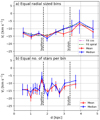 |
Fig. 4. Mean and median radial velocities relative to the sun as a function of distance d from the sun binned in 0.5 kpc bins (panel a), and in bins with 100 sources in each (panel b). Vertical lines indicate the locations of masers in the Sagittarius and Scutum arms. |
A weighted fit of the median values of the radial velocities toward the GC with the function Vr(d) = Av cos(2π(d − Dₒ)/lv) + Vₒ yields an amplitude Av = 3.4 ± 1.3km s−1, a maximum close to Dₒ = 4.0 ± 0.6 kpc, a wavelength lv = 4.8 ± 1.3 kpc, and a velocity offset Vₒ = −11.4 ± 1.2km s−1. Using a function for a logarithmic spiral Vr(d) = Av cos(ln(((R⊙ − d)/Rₒ)/tv) + Vₒ, we obtain Av = 3.9 ± 1.4km s−1, a maximum at ln(Rₒ/kpc) = 1.48 ± 0.08 with a scale tv = 0.13 ± 0.02, and an offset Vₒ = −10.7 ± 1.2km s−1. Amplitude and phase of the velocity variation are well determined; however, the wavelengths lv and tv depend critically on the last bins and are therefore less reliable. Furthermore, the wavelengths are likely to be underestimated due to the skewed error distribution of distances. The relative smooth variation of the median values as a function of radius suggests that the mass perturbation must have existed for a significant time as it otherwise could not have created such a regular velocity response. On the other hand, a more transient perturbation (Grand et al. 2015; Baba et al. 2018) cannot be excluded on the basis of the current data which only cover a small area of the Galactic plane.
To increase the radial resolution near the sun where the sources density is higher, bins with an equal number of sources were also used, as shown in Fig. 4b. This shows a general increase in the median velocity as a function of distance similar to that seen with fixed radial bins, but also two peaks at radii 1.7 kpc and 2.3 kpc. They are only marginally significant (i.e., at a 2–3σ level) and are reduced both if smaller or larger numbers of sources per bin are chosen. If they are real, they may be associated with minor mass concentrations in the vicinity of the Sagittarius arm. Furthermore, moving groups or stellar streams could be the origin since the stars have similar ages due to the distance–age correlation. The short distance between the peaks and their narrowness make it very unlikely that they are associated with a global density wave feature in the Galactic potential (e.g., a four-armed density wave is expected to have an inter-arm distance of at least 3 kpc).
A simple fit of an analytic function (e.g., a sinusoidal) does not account for possible nonlinear dynamical effects such as resonances. To include such nonlinear effects a grid of test-particle simulations was computed in a fixed axisymmetric potential with an imposed, density wave-like, spiral perturbation (Lin & Shu 1964; see Appendix A for details). Three spiral patterns were selected to agree with the observed locations of young sources in the Perseus arm at 9.9 kpc, the Sagittarius arm at 6.6 kpc, or the Scutum arm at 5.0 kpc (Reid et al. 2014; Wu et al. 2014). Two two-armed configurations were considered, one with arms corresponding to Perseus and Scutum with a pitch angle i = −12°̣3 (i.e., s2a) and the other using Perseus and Sagittarius as the major arms with i = −7°̣4 (i.e., s2b). For the four-armed model, a pattern going through the Perseus and Sagittarius arms with i = −14°̣5 was selected (i.e., s4a). In addition, models with a bar perturbation were computed with a bar mass equal to 10% of the bulge mass and a scale length of 4 kpc. The parameters for the models are summarized in Table 3 where m is the number of arms, ra the location of the next inner arm, Am the amplitude of the m-armed spiral, Ωb the bar pattern speed, while hb and nb are the bar shape parameters. Three two-armed models with a weaker m = 4 component were also considered to simulate the case of a higher harmonic response (i.e., sharper arms). Pattern speeds for the spirals were varied in the range 15–40 km s−1 kpc−1, while amplitudes up to 200 km2 s−2 were applied corresponding to a radial force perturbation relative to the axisymmetric field of dFr ≈ 6%. The models were integrated to a total time of 1 and 2 Gyr to ensure that an equilibrium was reached.
Parameters for the spiral potential models.
The radial velocity of the simulations were calculated in a polar coordinate system centered on the GC and with the phase θ increasing counterclockwise with zero in the direction toward the sun. To compare the simulations with the radial velocities measured, they were rebinned to match the data binned in equal radial bins (see first part of Table 2) and 2°̣8 in θ. The test variable ![$${T_{\rm{x}}}(\theta ) = \sum\nolimits_{n = 1}^{{N_{{\rm{bin}}}}} {{{([{V_{\rm{x}}}(n,\theta ) - {V^{\rm{m}}}(n) - {V_{\rm{o}}}]/\sigma ({V^{\rm{m}}}))}^2}} $$](/articles/aa/full_html/2018/11/aa33755-18/aa33755-18-eq8.gif) was computed where n is the radial bin, Nbin the number of bins, and x denotes the test-particle simulation including its amplitude and pattern speed. The value of Tx follows a χ2 distribution with Nbin − 2 degrees of freedom since the velocity offset Vo was estimated.
was computed where n is the radial bin, Nbin the number of bins, and x denotes the test-particle simulation including its amplitude and pattern speed. The value of Tx follows a χ2 distribution with Nbin − 2 degrees of freedom since the velocity offset Vo was estimated.
Acceptable models should have Tx < 9.12, which is the level estimated for models without spiral perturbations. Furthermore, the phase θm of the minimum Tx has to be close to zero in order to fit the distances observed for the Sagittarius or Scutum arm. The current distances to the arms refer to star-forming regions (e.g., masers), which may have an offset relative to the spiral potential minima. A phase offset of up to 30°, calculating 360° between arms, is possible if the star formation is concentrated close to a shock in the gas flowing through the spiral perturbation (Roberts 1969; Yuan & Grosbøl 1981; Gittins & Clarke 2004). Thus, models with |mθm| > 30θ should be rejected since they would not agree with the observed positions of star-forming regions in the arms defined by maser sources (Reid et al. 2014). Finally, the velocity offset Vo should be consistent with the solar peculiar motion of 11.1 km s−1 (Schönrich et al. 2010) within 3σ. The minimum Tx(|mθp| < 30°) values for models integrated to 1 Gyr are shown in Fig. 5 as a function of perturbation amplitude and pattern speed where the level of pure axisymmetric models is indicated by a dashed line. The actual values of Tx are listed in Table C.1 together with the velocity offset Vo and the phase of the minimum θm. The models integrated to 2 Gyr show very similar results.
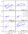 |
Fig. 5. Test variable Tx for models with phases |mθm| < 30° for the six models as a function of amplitude and pattern speed Ωp in km s−1 kpc−1. The horizontal dashed line indicates the Tx level for a model without spiral perturbations. |
The best models with these three criteria are two-armed spiral potentials with the Scutum arm as the next major, inner arm. Minimum Tx values are found for pattern speeds Ωp ≈ 20–30 km s−1 kpc−1 and amplitudes A2 ≈ 50 km2 s−2, which corresponds to dFr ≈ 1.5%. Two-armed models with an additional m = 4 harmonics (i.e., s2c–s2e) have slightly smaller Tx values. This corresponds to a slightly sharper spiral potential in azimuth. The amplitude of this m = 4 component depends on the steepness of the velocity profile near 4 kpc which is uncertain due to the small number of stars. Maps of relative surface density, radial velocity, and azimuthal velocity for the best model, s2c, with Ωp = 20 km s−1 kpc−1 and A2 = 40 km2 s−2 are shown in Fig. 6. This pattern speed places the 4:1 resonance region close to the solar radius which may explain some of the features seen in the velocity field in the solar neighborhood (Gaia Collaboration 2018b; Kawata et al. 2018; Antoja et al. 2018).
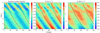 |
Fig. 6. Maps of the best test-particle simulation, s2c, with Ωp = 20 km s−1 kpc−1 and A2 = 40 km2 s−2: Panel a: relative surface density (normalized to unity in azimuth). Panel b: Vr = −v (i.e., positive for motion toward GC), and Panel c: Vθ. The imposed spiral potential minima are indicated by dashed lines. |
Although a few models with the Sagittarius as the next major arm (e.g., s2b and s4a) have Tx slightly smaller than a axisymmetric model, most of these models have |mθm| > 30° and can therefore be excluded. Models with an additional bar potential did not improve the match significantly as the main effect was a small shift of the radial velocities with no radial modulation except for resonance effects.
With Gaia DR2 proper motions, the tangential velocities of 1498 sources in the sample can be calculated using Johnson & Soderblom (1987) as seen in Fig. 7. The velocity component V in the direction of the Galactic rotation shows a flat distribution out to 2 kpc with 〈 V 〉 = −12.1 ± 0.8kms−1. At greater distances, a decline is seen due to the differential rotation of the Galaxy. A small peak near 2 kpc is consistent with the radial velocity variation, assuming a density wave perturbation (see Fig. 6c); however, the uncertainty on the Galactic rotation curve does not allow us to draw any conclusions. Similar variations are seen by Gaia Collaboration (2018b) and Kawata et al. (2018), also based on the Gaia DR2. The W component perpendicular to the Galactic plane also displayed a flat velocity distribution with 〈 W 〉 = 6.8 ± 0.5kms−1 to at least 2 kpc, after which a slow decline is observed. The lack of a significant variation in W makes it unlikely that the radial velocity changes observed are caused by an external source (i.e., a recent encounter with a dwarf galaxy) since such a perturber would also leave a trace in W velocities. The latter is likely an effect of the spatial distribution of the stars which are mainly located above the plane at large distances. The average values of all three velocity components are consistent with the solar peculiar motion relative to the LSR as determined by Schönrich et al. (2010).
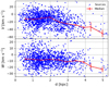 |
Fig. 7. Distribution of the velocity components V and W as a function of distance d from the sun. |
The U − V velocity distributions are shown in Fig. 8 grouped in radial bins. The closest bins display a marginal ellipsoidal distribution with angle offset of around 30° from the direction toward the GC, whereas the distributions at distances larger than 2.3 kpc become more circular. This may partly be due to the increasing errors in V as a function of distance. The angular offset is likely caused by the spiral perturbation which suggests that it is dynamically important to at least a distance of 3 kpc from the sun. Closer to the GC, interaction with the bar potential makes predictions uncertain. Some substructures can be seen in several bins (e.g., around 1.3 and 2.6 kpc). They may be caused by stellar streams or resonances, but the statistics are not sufficient for a detailed analysis.
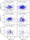 |
Fig. 8. U − V velocity ellipsoid as a function of distance d from the sun. |
5. Conclusion
The radial velocities of 1726 stars within 3° of the GC were measured with the FLAMES instrument at the VLT. The final sample consisted of 1507 sources with reliable velocities and distances (i.e., either from Gaia DR2 or main-sequence B-stars). The variation in the median radial velocities relative to the LSR as a function of distance from the sun shows a slow change from slightly negative values to a maximum close to 4 kpc. A least-squares fit of a sinusoidal function yields a velocity amplitude of 3.4±1.3kms−1 with a maximum at d = 4.0±0.6 kpc and a wavelength exceeding 4 kpc. This is consistent with the Scutum–Crux arm being the next major arm inside the sun. It should be noted that the velocity amplitude is likely to be underestimated as the average position of the stars is 40 pc from the plane. The larger number of sources close to the sun allowed a higher radial resolution which shows marginal velocity peaks at distances of 1.7 and 2.3 kpc. Although these peaks are in the range of the Sagittarius arm, their narrowness suggests that they are stellar streams near star-forming regions rather than global density wave-like perturbations. The mean radial velocity within 0.5 kpc of the arm is less than that of the LSR at a 99% level of confidence, which excludes it as a major, long-lived mass perturbation.
A fit of an analytic function to the velocity distribution does not account for possible nonlinear effects (e.g., resonances) which even at a relatively small amplitude may play a role. A set of test-particle simulations were computed in a fixed axisymmetric potential with imposed spiral and bar perturbations representing spiral patterns with either the Sagittarius or Scutum arm as the next major inner arm. The best agreement between the data and these models was found for a two-armed pattern having the Perseus and Scutum arms as major arms. Pattern speeds in the range of 20–30 km s−1 kpc−1 and amplitudes around 50 km2 s−2 (i.e., dFr ≈ 1.5%) were favored. Two-armed models with a sharper azimuthal perturbation (i.e., with an additional m = 4 harmonic term) gave slightly better fits, but depend on the shape of the velocity variation measured near 4 kpc, which is uncertain due to the small number of stars. The lifetime of the perturbation cannot be determined directly from the current data.
The current data suggest that the spiral potential of the Milky Way is two-armed with the Perseus and Scutum–Crux arms as majors. With a velocity amplitude of 3.4 km s−1 corresponding to dFr ≈ 1.5%, the perturbation is weak and in the linear domain (Grosbøl 1993). Marginal velocity peaks near the Sagittarius arm may be associated with star formation in the arm, but are too narrow to originate from a global perturbation. This favors a view of the Sagittarius arm as a weaker inter-arm feature with star formation excited either by the bar (Englmaier & Gerhard 1999, 2006) or a secondary shock (Yáñez et al. 2008).
Acknowledgments
We would like to acknowledge the detailed comments of the referee, which helped improve the paper. It is also a pleasure to thank Dr. V. Korchagin for useful and stimulating discussions. The ESO-MIDAS system and Python scripts with the SciPy package were used for the reduction and analysis of the data. This work has made use of data from the European Space Agency (ESA) mission Gaia (https://www.cosmos.esa.int/gaia), processed by the Gaia Data Processing and Analysis Consortium (DPAC, https://www.cosmos.esa.int/web/gaia/dpac/consortium). Funding for the DPAC has been provided by national institutions, in particular the institutions participating in the Gaia Multilateral Agreement.
References
- Antoja, T., Helmi, A., Romero-Góomez, M., et al. 2018, Nature, 561, 360 [NASA ADS] [CrossRef] [Google Scholar]
- Arenou, F., Luri, X., Babusiaux, C., et al. 2017, A&A, 599, A50 [NASA ADS] [CrossRef] [EDP Sciences] [Google Scholar]
- Baba, J., Kawata, D., Matsunaga, N., Grand, R. J. J., & Hunt, J. A. S. 2018, ApJ, 853, L23 [NASA ADS] [CrossRef] [Google Scholar]
- Bland-Hawthorn, J., & Gerhard, O. 2016, ARA&A, 54, 529 [NASA ADS] [CrossRef] [EDP Sciences] [Google Scholar]
- Block, D. L., Bertin, G., Stockton, A., et al. 1994, A&A, 288, 365 [NASA ADS] [Google Scholar]
- Bonnarel, F., Fernique, P., Bienaymé, O., et al. 2000, A&AS, 143, 33 [NASA ADS] [CrossRef] [EDP Sciences] [Google Scholar]
- Bressan, A., Marigo, P., Girardi, L., et al. 2012, MNRAS, 427, 127 [NASA ADS] [CrossRef] [Google Scholar]
- Carraro, G. 2015, BAAS, 57, 138 [Google Scholar]
- Carrillo, I., Minchev, I., Kordopatis, G., et al. 2018, MNRAS, 475, 2679 [NASA ADS] [CrossRef] [Google Scholar]
- Drimmel, R. 2000, A&A, 358, L13 [NASA ADS] [Google Scholar]
- Duchêne, G., & Kraus, A. 2013, ARA&A, 51, 269 [Google Scholar]
- Englmaier, P., & Gerhard, O. 1999, MNRAS, 304, 512 [NASA ADS] [CrossRef] [Google Scholar]
- Englmaier, P., & Gerhard, O. 2006, Celest. Mech. Dyn. Astron., 94, 369 [NASA ADS] [CrossRef] [Google Scholar]
- Eskridge, P. B., Frogel, J. A., Pogge, R. W., et al. 2002, ApJS, 143, 73 [NASA ADS] [CrossRef] [Google Scholar]
- Gaia Collaboration (Brown, A., et al.) 2016a, A&A, 595, A2 [NASA ADS] [CrossRef] [EDP Sciences] [Google Scholar]
- Gaia Collaboration (Prusti, T., et al.) 2016b, A&A, 595, A1 [NASA ADS] [CrossRef] [EDP Sciences] [Google Scholar]
- Gaia Collaboration (Brown, A., et al.) 2018a, A&A, 616, A1 [NASA ADS] [CrossRef] [EDP Sciences] [Google Scholar]
- Gaia Collaboration (Katz, D., et al.) 2018b, A&A, 616, A11 [NASA ADS] [CrossRef] [EDP Sciences] [Google Scholar]
- Gingerich, O. 1985, IAU Symp., 106, 59 [NASA ADS] [Google Scholar]
- Gittins, D. M., & Clarke, C. J. 2004, MNRAS, 349, 909 [NASA ADS] [CrossRef] [Google Scholar]
- Grand, R. J. J., Bovy, J., Kawata, D., et al. 2015, MNRAS, 453, 1867 [NASA ADS] [CrossRef] [Google Scholar]
- Grosbøl, P. 1993, PASP, 105, 651 [NASA ADS] [CrossRef] [Google Scholar]
- Grosbøl, P. 2016, A&A, 585, A141 [NASA ADS] [CrossRef] [EDP Sciences] [Google Scholar]
- Grosbøl, P., & Patsis, P. A. 1998, A&A, 336, 840 [NASA ADS] [Google Scholar]
- Hou, L. G., & Han, J. L. 2014, A&A, 569, A125 [NASA ADS] [CrossRef] [EDP Sciences] [Google Scholar]
- Husser, T.-O., von Berg, S. W., Dreizler, S., et al. 2013, A&A, 553, A6 [NASA ADS] [CrossRef] [EDP Sciences] [Google Scholar]
- Indebetouw, R., Mathis, J. S., Babler, B. L., et al. 2005, ApJ, 619, 931 [NASA ADS] [CrossRef] [Google Scholar]
- Johnson, D. R. H., & Soderblom, D. R. 1987, AJ, 93, 864 [NASA ADS] [CrossRef] [Google Scholar]
- Kawata, D., Baba, J., Ciucǎ, I., et al. 2018, MNRAS, 479, L108 [NASA ADS] [CrossRef] [Google Scholar]
- Lin, C. C., & Shu, F. H. 1964, ApJ, 140, 646 [NASA ADS] [CrossRef] [MathSciNet] [Google Scholar]
- Lin, C. C., Yuan, C., & Shu, F. H. 1969, ApJ, 155, 721 [NASA ADS] [CrossRef] [Google Scholar]
- Liszt, H. S. 1985, IAU Symp., 106, 283 [NASA ADS] [Google Scholar]
- Marigo, P., Girardi, L., Bressan, A., et al. 2017, ApJ, 835, 77 [NASA ADS] [CrossRef] [Google Scholar]
- Mark, J. W.-K. 1976, ApJ, 205, 363 [NASA ADS] [CrossRef] [Google Scholar]
- Monguió, M., Grosbøl, P., & Figueras, F. 2015, A&A, 577, A142 [NASA ADS] [CrossRef] [EDP Sciences] [Google Scholar]
- Palacios, A., Gebran, M., Josselin, E., et al. 2010, A&A, 516, A13 [NASA ADS] [CrossRef] [EDP Sciences] [Google Scholar]
- Pasquini, L., Avila, G., Blecha, A., et al. 2002, The Messenger, 110, 1 [NASA ADS] [Google Scholar]
- Reid, M. J., Menten, K. M., Brunthaler, A., et al. 2014, ApJ, 783, 130 [Google Scholar]
- Roberts, W. W. 1969, ApJ, 158, 123 [NASA ADS] [CrossRef] [Google Scholar]
- Rodríguez-Merino, L. H., Chavez, M., & Bertone, E. 2005, ApJ, 626, 411 [NASA ADS] [CrossRef] [Google Scholar]
- Russeil, D. 2003, A&A, 397, 133 [NASA ADS] [CrossRef] [EDP Sciences] [Google Scholar]
- Saito, R. K., Hempel, M., Minniti, D., et al. 2012, A&A, 537, A107 [NASA ADS] [CrossRef] [EDP Sciences] [Google Scholar]
- Schlafly, E. F., & Finkbeiner, D. P. 2011, ApJ, 737, 103 [NASA ADS] [CrossRef] [Google Scholar]
- Schönrich, R., Binney, J., & Dehnen, W. 2010, MNRAS, 403, 1829 [NASA ADS] [CrossRef] [Google Scholar]
- Shu, F. H. 1970, ApJ, 160, 99 [Google Scholar]
- Siebert, A., Famaey, B., Binney, J., et al. 2012, MNRAS, 425, 2335 [NASA ADS] [CrossRef] [Google Scholar]
- Visser, H. C. D. 1980a, A&A, 88, 149 [NASA ADS] [Google Scholar]
- Visser, H. C. D. 1980b, A&A, 88, 159 [NASA ADS] [Google Scholar]
- Wu, Y. W., Sato, M., Reid, M. J., et al. 2014, A&A, 566, A17 [NASA ADS] [CrossRef] [EDP Sciences] [Google Scholar]
- Yáñez, M. A., Norman, M. L., Martos, M. A., & Hayes, J. C. 2008, ApJ, 672, 207 [NASA ADS] [CrossRef] [Google Scholar]
- Yu, J., & Liu, C. 2018, MNRAS, 475, 1093 [NASA ADS] [CrossRef] [Google Scholar]
- Yuan, C., & Grosbøl, P. 1981, ApJ, 243, 432 [NASA ADS] [CrossRef] [Google Scholar]
Appendix A Galactic potential
Although it would be preferable to compute self-gravitating test-particle simulations, it is not currently feasible to initiate such models so that they generate a prescribed, stable spiral pattern. Thus, a set of test-particle simulations were calculated in a fixed galactic potential with an imposed spiral perturbation to estimate the velocity field of a stellar population with ages <2 Gyr. The axisymmetric potential consisted of three components: (1) a bulge with a Kuzmin potential with a total mass of 1.8 × 10⁹ M⊙ and a scale length of 1.0 kpc, (2) an exponential disk with a central surface density of 573.0 M⊙ pc−2 and a scale length of 2.5 kpc, and (3) a logarithmic potential for the halo with a maximum velocity of 220 km s−1 and a scale length of 2.0 kpc. This potential is consistent with the Milky Way model of Bland-Hawthorn & Gerhard (2016) and has a rotational speed of 244 km s−1 at the solar radius R⊙ = 8.36 kpc (Reid et al. 2014).
Although the length of the Galactic bar is less than 5 kpc (Bland-Hawthorn & Gerhard 2016), it may still affect the stellar velocity field at larger distances due to its quadruple moment. Thus, a bar potential with a pattern speed different from that of the spiral was included. The spiral perturbation was not truncated in the bar region which leads to an unrealistic potential in the very inner parts of the Galaxy. This is not an issue since the major objective of the models is to estimate the velocity field between the sun and the Scutum arm, which must be outside the bar region.
The models were populated with 2 × 10⁷ test particles in the radial range of 3.5–9.5 kpc from the GC with a uniform distribution in azimuth and a radial surface density variation given by the disk surface density. Due to the symmetry of the models, there are twice as many effective particles. The particles were given energies corresponding to circular orbits, while their velocity dispersion followed a Gaussian distribution with a dispersion of 10 km s−1. The amplitude of spiral and bar potentials was increased linearly from zero to the specified values over the first 0.6 Gyr, after which they were kept constant. The orbits of the particles were integrated to an age of 1 and 2 Gyr using a 4th-order Runge-Kutta predictor-corrector method with variable step ensuring a relative error of less than 10−6. This allows the models to be dynamically relaxed, but still have ages comparable to those of the stars measured.
The model of the Galactic potential Φ consists of the sum of three part and depends on radius r, phase θ, and time t

where Φ0 is the axisymmetric term; Φs is the spiral potential, which has no time dependence since the frame of reference is rotating with the angular speed of Ωp; and the last term Φb represents the bar potential, which may rotate with a different speed and therefore is dependent on time.
The axisymmetric potential has three terms representing a bulge (A.2), an exponential disk (A.3), and a halo (A.4),


where y = 0.5r/hd and G is the gravitational constant. The bulge was defined by its mass MB = 1.8 109 M⊙ and scale length hB = 1.0 kpc. The exponential disk had a central surface density Σd = 573 M⊙ pc−2 and a scale length hd = 2.5 kpc where the functions I and K are the Bessel functions. The halo had a maximum rotational speed of Vh = 220 km s−1 and the scale length hh = 2 kpc.
The spiral potential is defined by

where m is the number of arms, i is the pitch angle, and As is the amplitude. A scale length hs = 6.0 kpc was used to ensure a small radial variation of the radial force introduced by the spiral relative to the axisymmetric force.
The bar potential was allowed to rotate with a different angular speed Ωb compared to that of the reference frame Ωp and had the form

where Ab, θb, and hb are amplitude, initial phase, and scale length, respectively. The bar shape was determined by nb which was set to 4 giving a relative fast decline of the potential with radius. Models with nb = 2 or 6 were also computed, but showed no significant differences at the distances relevant for the current data. The amplitude was fixed to 10% of the bulge mass, i.e., Mb = 1.8 × 10⁸ M⊙ , while the scale length hb was set to 4 kpc. The exact analytical shape of the bar potential is not essential for the response at distances significant outside the bar region where the bar quadruple moment provides the main effect.
The Hamiltonian H of the system rotating with the angular speed Ωp is given as

where v is the radial velocity and J the angular momentum. The energy is only preserved for Ab = 0.
Models with pattern speeds Ωp in the range 15–40 km s−1 kpc−1 were computed, which placed the major resonances at the radii listed in Table A.1.
Distance from GC in kpc of stellar resonances in the axisymmetric potential as a function of pattern speed Ωp in km s−1 kpc−1.
Appendix B Catalog of radial velocities
The catalog of the observed radial velocities of stars with S/N > 10 is available through CDS as a FITS table with the columns listed in Table B.1. Values for log(g) and spectroscopic distances, d-spec, are given only for main-sequence B-stars, i.e., log(Teff) > 4.0 and log(g) > 3.5.
Column specifications for FITS table with radial velocity data.
Appendix C Probabilities for models
The test variables Tx for the observed radial velocity distribution to be taken from the distributions computed from the test-particle simulations are listed in the Table C.1. The model name is given together with pattern speed Ωp in km s−1 kpc−1, spiral amplitude in km2 s−2, velocity offset relative to the sun Vo in km s−1, phase offset θm in degrees, and the test variable Tx. Only models with Tx < 9.12 (i.e., less than that for a pure axisymmetric models), |Vo − 11.1| < 2.1 km s−1, and |mθm| < 30° are included.
List of test variables Tx for test-particle simulations with a value less than that of an unperturbed model.
All Tables
List of the number of sources N, mean velocity , standard deviation σ(Vr), and median velocity in km s−1 including their errors in distance bins centered on d (kpc).
Distance from GC in kpc of stellar resonances in the axisymmetric potential as a function of pattern speed Ωp in km s−1 kpc−1.
List of test variables Tx for test-particle simulations with a value less than that of an unperturbed model.
All Figures
|
Fig. 1. Distribution of sources as a function of their effective temperature Teff. The upper diagram gives the histogram of sources while the lower one shows the signal-to-noise ratio (S/N) both in logarithmic scale. |
| In the text | |
|
Fig. 2. Distances from Gaia DR2 parallaxes as a function of the distances determined from the spectra observed for stars with 4.0 < log(Teff). Stars with log(g) < 3.5 are indicated by crosses. |
| In the text | |
|
Fig. 3. Near-infrared extinction A(Ks) and barycentric radial velocity Vr as a function of distance d from the sun. |
| In the text | |
|
Fig. 4. Mean and median radial velocities relative to the sun as a function of distance d from the sun binned in 0.5 kpc bins (panel a), and in bins with 100 sources in each (panel b). Vertical lines indicate the locations of masers in the Sagittarius and Scutum arms. |
| In the text | |
|
Fig. 5. Test variable Tx for models with phases |mθm| < 30° for the six models as a function of amplitude and pattern speed Ωp in km s−1 kpc−1. The horizontal dashed line indicates the Tx level for a model without spiral perturbations. |
| In the text | |
|
Fig. 6. Maps of the best test-particle simulation, s2c, with Ωp = 20 km s−1 kpc−1 and A2 = 40 km2 s−2: Panel a: relative surface density (normalized to unity in azimuth). Panel b: Vr = −v (i.e., positive for motion toward GC), and Panel c: Vθ. The imposed spiral potential minima are indicated by dashed lines. |
| In the text | |
|
Fig. 7. Distribution of the velocity components V and W as a function of distance d from the sun. |
| In the text | |
|
Fig. 8. U − V velocity ellipsoid as a function of distance d from the sun. |
| In the text | |
Current usage metrics show cumulative count of Article Views (full-text article views including HTML views, PDF and ePub downloads, according to the available data) and Abstracts Views on Vision4Press platform.
Data correspond to usage on the plateform after 2015. The current usage metrics is available 48-96 hours after online publication and is updated daily on week days.
Initial download of the metrics may take a while.