| Issue |
A&A
Volume 619, November 2018
|
|
|---|---|---|
| Article Number | A62 | |
| Number of page(s) | 5 | |
| Section | Galactic structure, stellar clusters and populations | |
| DOI | https://doi.org/10.1051/0004-6361/201833723 | |
| Published online | 09 November 2018 | |
Exploring the space density of X-ray selected cataclysmic variables
Leibniz-Institut für Astrophysik Potsdam (AIP), An der Sternwarte 16, 14482 Potsdam, Germany
e-mail This email address is being protected from spambots. You need JavaScript enabled to view it.
Received:
26
June
2018
Accepted:
21
August
2018
Abstract
The space density of the various classes of cataclysmic variables (CVs) has up to now only been weakly constrained, due to the small number of objects in complete X-ray flux-limited samples and the difficulty in deriving precise distances to CVs. The former limitation still exists. Here the impact of Gaia parallaxes and implied distances on the space density of X-ray-selected complete, flux-limited samples is studied. These samples have been described in the literature: Those of non-magnetic CVs are based on ROSAT (RBS – ROSAT Bright Survey & NEP – North Ecliptic Pole) and that of the intermediate polars (IPs) stems from Swift/BAT. All CVs appear to be rarer than previously thought, although the new values are all within the errors of past studies. Upper limits at 90% confidence for the space densities of non-magnetic CVs are ρRBS < 1.1 × 10⁻⁶ pc−3 and ρRBS+NEP < 5.1 × 10⁻⁶ pc−3 for an assumed scale height of h = 260 pc and ρIPs < 1.3 × 10⁻⁷ pc−3 for the long-period IPs at a scale height of 120 pc. Most of the distances to the IPs have previously been under-estimated. The upper limits to the space densities are only valid in cases where CVs do not have lower X-ray luminosities than the lowest-luminosity member of the sample. These results require confirmation using larger sample sizes, soon to be established through sensitive X-ray all-sky surveys to be performed with eROSITA on the Spektrum-X-Gamma mission.
Key words: novae, cataclysmic variables / surveys / X-rays: binaries
© ESO 2018
1. Introduction
The space density of cataclysmic variable stars (CVs) is one of the bigger unknowns in the field. Being the outcome of binary star evolution through a common envelope and subsequent angular momentum loss, this value is important for several parameters and processes that are relevant to binary evolution, including the initial binary separation, the initial mass distribution, the common envelope efficiency, and the angular momentum loss in the post-common envelope phase and that in the CV stage. It is the most relevant value to compare with binary population synthesis. The simple question is: how many CVs are out there?
This question is relevant for stellar evolution but has implications for models of the total energy output of the Milky Way. One of the contenders to explain the infamous Galactic ridge X-ray emission (GRXE, Worrall et al. 1982) is CVs and in particular magnetic CVs of the intermediate polar type (IPs). Through a deep Chandra pointing close to the galactic centre, the apparently diffuse GRXE was largely resolved into point sources (Revnivtsev et al. 2009). The composition however remained uncertain and was discussed thoroughly in the recent past and sensitively depends on the space density and the luminosity functions of the main source classes (e.g. Warwick 2014; Nobukawa et al. 2016).
The second data release from the Gaia satellite (Gaia DR2) opens the opportunity to re-assess the space density of X-ray-selected cataclysmic variables. Past studies were hampered by small sample sizes and imprecisely determined distances. While the former limitation cannot presently be overcome, the latter has essentially vanished.
In this paper the non-magnetic CVs (dwarf nova and nova-like systems) and one class of the magnetic CVs, the IPs, are addressed. Both sub-classes have relatively well-understood X-ray spectra which results in a relatively clean selection of objects. The strongly magnetic CVs, the polars, are not addressed here. Polars are special due to their more complex X-ray spectra with a thermal plasma and a potentially strong soft component. ROSAT has uncovered many soft blackbody-like polars (Beuermann & Schwope 1994), but all new discoveries made with XMM-Newton lack the pronounced soft component (see e.g. Webb et al. 2018, and references therein). Whether or not the observed sample of polars can be regarded as representative of the parent population is therefore questionable.
2. Analysis
2.1. Basic assumptions
In the following we derive space densities for X-ray-selected samples of CVs. The samples are described in the literature and no new sample composition was undertaken. We make three basic assumptions per case: that the observed sample is representative of the intrinsic population, the sample is complete, and that the sample is flux-limited with a well-defined flux-limit. For further details, see for example Pretorius & Knigge (2012).
For the analyses in the following sections we make use of parallaxes that were found by archival cone searches in the Gaia archive using data from Gaia DR21. In case of multiple matches, the entry with the best matching brightness value was chosen. We do not invert parallaxes to infer distances but use the probabilistic distance estimates provided by Bailer-Jones et al. (2018)2. However, since most new parallaxes have very small relative errors, the use of directly inverted parallaxes gives almost the same results.
2.2. The V/Vmax method
We follow the approach used earlier (e.g. Hertz et al. 1990; Schwope et al. 2002; Pretorius et al. 2007) to estimate the space density of CVs using a V/Vmax method. Since many of the CVs used here are at high galactic latitude and some of them are at a distance in excess of the likely scale height of CVs, we use the modified method by Tinney et al. (1993). This method of calculation of a generic volume, Vgen, accounts for an exponential density distribution ρ ∝ exp[(−d| sin b|)/h] (d: distance, b: galactic latitude, h: galactic scale height). Vgen is calculated by
 (1)
(1)
with ξ = d| sin b|/h and Ω the solid angle of the survey. The maximum generic volume Vgen is computed using this formula with the maximum possible distance of the particular source which would allow its detection at the flux limit of the survey. One particular CV then contributes 1/Vgen to the space density ρX, that is, the space density is
 (2)
(2)
The derived numbers per object are given in the tables below.
Per observed sample one needs to specify the flux limit, which determines the maximum distance for an object still to be detected, the scale height of the distribution, and the solid angle of the survey.
Using Gaussian distributed parallax and flux errors per object, 90% confidence regions for the derived ρ per sample and per assumed scale height were computed by running approximately 50,000 simulated mock samples per case. The results with their confidence ranges are listed in Table 4.
X-ray luminosities in this paper are always computed via LX = 4πD2FX without any possible geometric correction factor. This leads to the revised luminosities given in the tables below.
2.2.1. The RBS sample of non-magnetic CVs
The ROSAT-sample of non-magnetic CVs described in Schwope et al. (2002) was drawn from the ROSAT Bright Survey (RBS, Schwope et al. 2000), an identification programme of all high-galactic latitude sources found in the RASS. It reached an identification rate as high as 99.7%. Based on the identification of two apparently close, low-luminosity systems, RBS0490 and RBS1955, Schwope et al. (2002) derived a space density of ~3 × 10⁻⁵ pc−3. Due to their assumed proximity they were the dominating terms in the sum of Eq. (2). When the two objects were removed from their sample, the density became ρX,RBS = 1.5 × 10⁻⁶ pc−3.
Triggered by this study, Thorstensen et al. (2006, 2009) revised the distances to RBS0490 and RBS1955 to ~300 pc and  pc, respectively, thus favouring the lower value of ρ which was later confirmed by Pretorius & Knigge (2012).
The original list of RBS-CVs is given in Table 1. For a re-determination of the space density some updates are necessary. Firstly, RBS0713 (=EI UMa) is now regarded as being an IP (Baskill et al. 2005) and will not be included in the analysis. On the other hand RBS0664 was regarded as an IP previously and was re-classified as a non-magnetic CV by Pretorius & Knigge (2012).
Non-magnetic CVs found in the RBS.
Secondly, the RASS was recently reprocessed by Boller et al. (2016) and count rates were updated. We read the revised count rates from the online version of the catalogue3 and convert those to fluxes using the same ECF (energy to count conversion factor) as in Schwope et al. (2002), ECF = 1.41 × 10⁻¹¹ erg cm−2 s−1/count.
Gaia distances are also listed in Table 1. All but one have errors <5%. The only exception, RBS1411, has a relative uncertainty of 23%.
The corresponding numbers for Vgen are listed in Table 1 together with the X-ray flux, the parallax (plus error), the estimated distance and the maximum distance that was used to compute the generic volume. The survey area used was 20 400 deg2.
Here and in the other subsections the generic volume was computed for three different scale heights, that is, those that were used in the original publications: 200 pc for the RBS-CVs, 260 pc for the RASS-CVs, and 120 pc for the IPs. All derived space densities are listed in Table 4.
A few of the non-magnetic RBS-CVs might have an uncertain classification, and therefore a final composition of the sample is subject to changes if newer information becomes available. One example is RBS1955 which is difficult to classify and could well be a magnetic CV (Schwope et al. 2014); if removed from the sample, one obtains a density 10% lower than that given in Table 4.
2.2.2. The RASS (RBS and NEP) sample of non-magnetic CVs
Pretorius & Knigge (2012) used the non-magnetic RBS-CVs and added four CVs from the ROSAT-NEP (North Ecliptic Pole, Pretorius et al. 2007) survey to study the space density and the X-ray luminosity function of CVs. They re-considered all distance determinations used previously to obtain  for an assumed scale height of 260 pc. Their error budget is based on Monte-Carlo simulations of the probability distribution function that find ρ for a large number of mock samples with properties that fairly sample the parameter space allowed by the data.
The list of objects with their newly determined distances, luminosities, and other parameters is given in Table 2. The survey area used is 20 400 deg2 at a limiting flux of 1.1 × 10⁻¹² erg cm−2 s−1 for the RBS part and 81 deg2 for the NEP part of the sample.
Non-magnetic CVs used by Pretorius & Knigge (2012) to obtain the space density of RASS-selected objects.
As a test for consistency we re-calculated the space density using their data as far as we were able to recover those. The limiting flux is not constant over the NEP area and Pretorius et al. (2007) describe how to correctly deal with the variable flux limit. It is not expected that the correct treatment makes a significant difference to the results achieved here. Following Henry et al. (2006) we therefore simply used the same limit of 2 × 10⁻¹⁴ erg cm−2 s−1 for the NEP survey area to obtain ρX,RASS = 4.1 × 10⁻⁶ pc−3 as a reference value assuming the same scale height of h = 260 pc as in Pretorius & Knigge (2012).
Pretorius & Knigge (2012) used a slightly different X-ray band to Schwope et al. (2002) and corrected their fluxes for interstellar extinction which explains the different derived values of ρX despite using the same objects. As we show below, the differences are small compared to other parameters affecting ρ. We therefore tested the influence of the sample composition and different flux convention used by Schwope et al. (2002) and Pretorius & Knigge (2012) by removing the four NEP-CVs from the RASS-sample and re-computing the space density. The results are listed in Table 4 in the row labelled “RASS (RBS-part)”.
2.2.3. The sample of intermediate polars from the Swift/BAT 70 month survey
The third sample to be studied here is the Swift/BAT sample of IPs presented by Pretorius & Mukai (2014). They list 15 IPs that were observed in the energy range 14–195 keV. This band is not affected by galactic foreground absorption. The limiting flux of this survey is FX = 2.5 × 10⁻¹¹ erg cm−2 s−1 and the survey was restricted to galactic latitudes bII > |5|°. The space density derived for long-period IPs with an assumed scale height of 120 pc was  .
.
The IPs used in this exercise with their newly determined distances and luminosities are listed in Table 3.
Intermediate polars used by Pretorius & Mukai (2014) to obtain the space density.
XY Ari is behind a dark cloud and has no optical counterpart, and is therefore without data from Gaia. We use the same distance as Pretorius & Mukai (2014). V2731 Oph has a relative parallax error of 13%, and V1062 Tau a relative error of 12%. Most other parallax errors are below 3%.
3. Results and discussion
The space densities of X-ray-selected samples of magnetic and non-magnetic CVs was redetermined using recently published parallaxes and distances from Gaia DR2. The results are summarized in Table 4 and Figs. 1 and 2. Figure 2 shows distributions of the original and the revised luminosities found for the RASS-CVs and the IPs, while Fig. 1 shows the weight per object (inverse of the generic volume) over its luminosity.
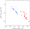 |
Fig. 1. Scatter plot showing the X-ray luminosities and the weights (inverse of the generic volumes) per object studied here. The Swift/BAT selected IPS are shown in red for a scale height of 120 pc, the RASS CVs are shown in blue, and the NEP-CVs in the RASS sample in cyan. Assumed scale height for RASS-CVs was 260 pc. |
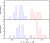 |
Fig. 2. Published (upper panel, adapted from Pretorius & Knigge 2012; Pretorius & Mukai 2014) and revised (lower panel) luminosity distributions of the RASS-CVs (blue-shaded histogram) and the Swift/BAT-selected IPs (red). The bin width is 0.2 dex. |
Space densities of the X-ray-selected CV samples as a function of assumed scale height.
Just as a reference, the published values of ρ for the RBS, the RASS, and the IP samples were  ,
,  and
and  , for scale heights of 200 pc, 260 pc, and 120 pc, respectively (Schwope et al. 2002; Pretorius & Knigge 2012; Pretorius & Mukai 2014). The comparison with the values listed in Table 4 shows that all newly derived densities are smaller than published ones but still within the published errors.
The statistical errors of ρ of the non-magnetic CVs could be reduced very significantly thanks to precise Gaia data. The statistical error of ρ for the IP sample is still large due to the shallow flux limit.
For the RBS-CVs, the space density is safely below 1.8 × 10⁻⁶ pc−3 at 90% confidence but could be smaller than 1.1 × 10⁻⁶ pc−3 if the scale height were found to be as high as 260 pc as assumed by Pretorius & Knigge (2012). This result remains unchanged if the fluxes in the band 0.5−2.0 keV are used (third row in Table 4). The RBS-sample consists of long- and short-period CVs. It therefore appears possible that not all objects belong to the same galactic population. The use of just one scale to characterise the sample is likely an oversimplification.
The RASS-CVs (RBS+NEP) are compatible with a significantly higher space density thanks to the lower flux limit of the NEP. The inclusion of just four CVs from the NEP-survey implies a space density that is larger than without this inclusion by a factor ranging from 4 to 7. Figure 1 illustrates that at a given luminosity each of those CVs has a higher weight than a corresponding RBS-CV by a factor of approximately ten. The whole sample is dominated by just one CV, the low-luminosity object EX Dra, log LX = 29.8 erg s−1, a rather unhealthy situation for the whole analysis.
The pre-Gaia distances of the RASS-CVs were quite reliable, hence the median X-ray luminosity of the RASS sample remained unchanged at log LX = 31.2 erg s−1. The distribution of luminosities is less dispersed in the centre but slightly more fuzzy at the outskirts (Fig. 4). The standard deviation of log LX was 0.54 dex and is now 0.57 dex; omitting the highest and lowest values it was 0.46 dex and is now 0.38 dex.
For the IPs, the first important thing to note is that all but one object, GK Per, have larger distances than previously assumed. They are therefore more luminous than thought; the median luminosity is shifted from log LX = 33.1 erg s−1 to 33.5 erg s−1. Furthermore, the survey volume becomes larger and the space density conversely smaller. An upper limit to the space density of the IPs is ρ < 1.3 × 10⁻⁷ pc−3 at 90% confidence, a significant reduction compared to the published value. The most likely value at  is at 74% of the published one.
Distances to the IPs used by Pretorius & Mukai (2014) were either taken from the literature (3 trigonometric and 4 photometric parallaxes from the donor star) or were newly determined and based on WISE IR-magnitudes combined with the semi-empirical donor sequence by Knigge (2006). Not surprisingly, the mean distance ratio new/old is reasonably small: drat = 1.12 for the three IPs which previously had a trigonometric parallax – among them GK Per with a Gaia distance smaller than published. The IPs with photometric parallaxes of the donor have drat = 1.33 and those with estimated distances from WISE and the empirical donor sequence have a mean ratio drat = 1.74. This leaves the two possibilities that either the IR donor sequence is somehow biased or that an additional emission component (dust, cyclotron radiation, free-free emission) mimics brighter secondaries.
Otherwise the IP sample appears more homogeneous than the sample of non-magnetic CVs. There is not one object or subgroup of objects that dominates the space density. However, given the relatively high flux limit the number for ρ derived here is valid only for the potentially rare objects with high luminosities. The putative class of low-luminosity IPs remains to be uncovered (see e.g. Worpel et al. 2018).
This present study provides an update on the space density of X-ray-selected CVs. Cataclysmic variables appear to be rarer than previously thought. While the limitations due to uncertain distances are overcome thanks to Gaia, major obstacles remain preventing further progress. These are the small sample sizes that are due to shallow flux limits of past X-ray surveys and a lack of information regarding the proper scale heights of the samples. It also appears likely that the existing samples are inhomogeneously composed as far as their scale height is concerned; they contain long-and short-period objects. Further, some of them lack determinations of their orbital period, which could be used to assign class membership, that is, membership of an older or younger population with corresponding scale height. The limitation caused by the small sample sizes will hopefully soon be overcome as a result of the upcoming eROSITA all-sky surveys (Merloni et al. 2012; Schwope 2012) with an all-sky flux limit comparable to the ROSAT-NEP survey but with enlarged energy coverage, 0.3−10 keV, and better spatial resolution compared to ROSAT. Performing the survey is just the first step on a longer journey, eventually involving spectroscopic identification, classification, and detailed follow-up to determine orbital periods.
Acknowledgments
I thank Fabian Emmerich for help with type-setting and Hauke Wörpel for useful hints regarding Gaia distances. I thank an anonymous referee whose comments helped to improve the quality and clarity of the paper. This work has made use of data from the European Space Agency (ESA) Gaia (https://www.cosmos.esa.int/gaia), processed by the Gaia Data Processing and Analysis Consortium (DPAC, https://www.cosmos.esa.int/web/gaia/dpac/consortium). Funding for the DPAC has been provided by national institutions, in particular the institutions participating in the Gaia Multilateral Agreement.
References
- Bailer-Jones, C. A. L., Rybizki, J., Fouesneau, M., Mantelet, G., & Andrae, R. 2018, AJ, 156, 58 [NASA ADS] [CrossRef] [Google Scholar]
- Baskill, D. S., Wheatley, P. J., & Osborne, J. P. 2005, MNRAS, 357, 626 [NASA ADS] [CrossRef] [Google Scholar]
- Beuermann, K., & Schwope, A. D. 1994, ASP Conf. Ser., 56, 119 [NASA ADS] [Google Scholar]
- Boller, T., Freyberg, M. J., Trümper, J., et al. 2016, A&A, 588, A103 [NASA ADS] [CrossRef] [EDP Sciences] [Google Scholar]
- Henry, J. P., Mullis, C. R., Voges, W., et al. 2006, ApJS, 162, 304 [NASA ADS] [CrossRef] [Google Scholar]
- Hertz, P., Bailyn, C. D., Grindlay, J. E., et al. 1990, ApJ, 364, 251 [NASA ADS] [CrossRef] [Google Scholar]
- Knigge, C. 2006, MNRAS, 373, 484 [NASA ADS] [CrossRef] [Google Scholar]
- Merloni, A., Predehl, P., Becker, W., et al. 2012, ArXiv e-prints [arXiv:1209.3114] [Google Scholar]
- Nobukawa, M., Uchiyama, H., Nobukawa, K. K., Yamauchi, S., & Koyama, K. 2016, ApJ, 833, 268 [NASA ADS] [CrossRef] [Google Scholar]
- Pretorius, M. L., & Knigge, C. 2012, MNRAS, 419, 1442 [NASA ADS] [CrossRef] [Google Scholar]
- Pretorius, M. L., & Mukai, K. 2014, MNRAS, 442, 2580 [NASA ADS] [CrossRef] [Google Scholar]
- Pretorius, M. L., Knigge, C., O’Donoghue, D., et al. 2007, MNRAS, 382, 1279 [NASA ADS] [CrossRef] [Google Scholar]
- Revnivtsev, M., Sazonov, S., Churazov, E., et al. 2009, Nature, 458, 1142 [NASA ADS] [CrossRef] [PubMed] [Google Scholar]
- Schwope, A. 2012, Mem. Soc. Astron. It., 83, 844 [NASA ADS] [Google Scholar]
- Schwope, A., Hasinger, G., Lehmann, I., et al. 2000, Astron. Nachr., 321, 1 [NASA ADS] [CrossRef] [Google Scholar]
- Schwope, A. D., Brunner, H., Buckley, D., et al. 2002, A&A, 396, 895 [NASA ADS] [CrossRef] [EDP Sciences] [Google Scholar]
- Schwope, A. D., Scipione, V., Traulsen, I., et al. 2014, A&A, 561, A121 [NASA ADS] [CrossRef] [EDP Sciences] [Google Scholar]
- Thorstensen, J. R., Lépine, S., & Shara, M. 2006, PASP, 118, 1238 [NASA ADS] [CrossRef] [Google Scholar]
- Thorstensen, J. R., Schwarz, R., Schwope, A. D., et al. 2009, PASP, 121, 465 [NASA ADS] [CrossRef] [Google Scholar]
- Tinney, C. G., Reid, I. N., & Mould, J. R. 1993, ApJ, 414, 254 [NASA ADS] [CrossRef] [Google Scholar]
- Warwick, R. S. 2014, MNRAS, 445, 66 [NASA ADS] [CrossRef] [Google Scholar]
- Webb, N. A., Schwope, A., Zolotukhin, I., Lin, D., & Rosen, S. R. 2018, A&A, 615, A133 [NASA ADS] [CrossRef] [EDP Sciences] [Google Scholar]
- Worpel, H., Schwope, A., Traulsen, I., Mukai, K., & Ok, S. 2018, A&A, 617, A52 [NASA ADS] [CrossRef] [EDP Sciences] [Google Scholar]
- Worrall, D. M., Marshall, F. E., Boldt, E. A., & Swank, J. H. 1982, ApJ, 255, 111 [NASA ADS] [CrossRef] [Google Scholar]
All Tables
Non-magnetic CVs used by Pretorius & Knigge (2012) to obtain the space density of RASS-selected objects.
Intermediate polars used by Pretorius & Mukai (2014) to obtain the space density.
Space densities of the X-ray-selected CV samples as a function of assumed scale height.
All Figures
|
Fig. 1. Scatter plot showing the X-ray luminosities and the weights (inverse of the generic volumes) per object studied here. The Swift/BAT selected IPS are shown in red for a scale height of 120 pc, the RASS CVs are shown in blue, and the NEP-CVs in the RASS sample in cyan. Assumed scale height for RASS-CVs was 260 pc. |
| In the text | |
|
Fig. 2. Published (upper panel, adapted from Pretorius & Knigge 2012; Pretorius & Mukai 2014) and revised (lower panel) luminosity distributions of the RASS-CVs (blue-shaded histogram) and the Swift/BAT-selected IPs (red). The bin width is 0.2 dex. |
| In the text | |
Current usage metrics show cumulative count of Article Views (full-text article views including HTML views, PDF and ePub downloads, according to the available data) and Abstracts Views on Vision4Press platform.
Data correspond to usage on the plateform after 2015. The current usage metrics is available 48-96 hours after online publication and is updated daily on week days.
Initial download of the metrics may take a while.