| Issue |
A&A
Volume 619, November 2018
|
|
|---|---|---|
| Article Number | A54 | |
| Number of page(s) | 7 | |
| Section | Stellar structure and evolution | |
| DOI | https://doi.org/10.1051/0004-6361/201833352 | |
| Published online | 07 November 2018 | |
Fast and slow winds from supergiants and luminous blue variables
1 Armagh Observatory and Planetarium, College Hill, Armagh BT61 9DG, UK
e-mail: This email address is being protected from spambots. You need JavaScript enabled to view it.
2 Kavli Institute for Theoretical Physics, University of California, Santa Barbara, CA 93106, USA
Received:
3
May
2018
Accepted:
20
August
2018
Abstract
We predict quantitative mass-loss rates and terminal wind velocities for early-type supergiants and luminous blue variables (LBVs) using a dynamical version of the Monte Carlo radiative transfer method. First, the observed drop in terminal wind velocity around spectral type B1 is confirmed by the Monte Carlo method at the correct effective temperature of about 21 000 K. This drop in wind velocity is much steeper than would be expected from the drop in escape speed for cooler stars. The results may be particularly relevant for slow winds inferred for some high-mass X-ray binaries. Second, the strength of the mass-loss bi-stability jump is found to be significantly greater than previously assumed. This could this make bi-stability braking more efficient in massive star evolution; in addition, a rotationally induced version of the bi-stability mechanism may now be capable of producing the correct density of outflowing disks around B[e] supergiants, although multi-dimensional modelling including the disk velocity structure is still needed. For LBVs we find that the bi-stability jump becomes larger at higher metallicities, but perhaps surprisingly also larger at lower Eddington parameters. This may have consequences for the role of LBVs in the evolution of massive stars at different metallicities and cosmic epochs. Finally, our predicted low wind velocities may be important for explaining the slow outflow speeds of supernova type IIb/IIn progenitors, for which the direct LBV-SN link was first introduced.
Key words: radiation: dynamics / stars: variables: S Doradus / stars: early-type / supergiants / stars: mass-loss
© ESO 2018
1. Introduction
Mass loss is an important driver of massive star evolution (Chiosi & Maeder 1986; Langer 2012). This is thought to occur via stationary stellar winds on and off the main sequence (Vink & Gräfener 2012; Groh et al. 2014), and possibly also in eruptive mode during luminous blue variable (LBV) events (Shaviv 2000; Smith & Owocki 2006; Owocki 2015). Although detailed stationary wind models of LBVs have been constructed by Vink & de Koter (2002) using the Abbott & Lucy (1985) Monte Carlo radiative transfer approach, the predicted mass-loss rates (Ṁ) were semi-empirical in nature, and assumed terminal wind velocities (v∞). Dynamical modelling has yet to be explored. In this paper, we will employ the dynamically consistent approach of Müller & Vink (2008) to predict velocity structures and mass-loss rates for a range of OB supergiants and LBV models, as well as their metallicity (Z) dependence.
Pauldrach & Puls (1990) first encountered the bi-stability jump in modelling the wind of the LBV P Cygni. Lamers et al. (1995) subsequently found observational evidence for the bi-stability jump through a drop in wind velocities by a factor of two for a sample of supergiants around spectral type B1 at an effective temperature of about 21 000 K (see also Crowther et al. 2006). It was originally assumed that the jump was caused by the optical depth of the Lyman continuum, until Vink et al. (1999) showed that the recombination of the main line-driving element iron (Fe) caused an increased amount of line acceleration from Fe III – and an increase in the mass-loss rate by a factor of five. As these models were semi-empirical in nature, the drop in terminal wind velocity has yet to be theoretically modelled.
The issue of whether the mass-loss rate increases at the bi-stability location, as predicted, or whether it drops instead, as suggested by empirical results (Trundle et al. 2004; Crowther et al. 2006; Benaglia et al. 2007; Markova & Puls 2008; Morford et al. 2016), remains unresolved, and may depend on the question of whether the discrepancy can be attributed to macro-clumping, as Petrov et al.(2014) showed that the Hα line changes its character completely from an optically thin to an optically thick line below the bi-stability jump.
In the current paper, we present new dynamically consistent mass-loss predictions on both sides of the bi-stability jump, and we find that we are indeed able to confirm the observed drop in terminal wind velocities. Moreover, we predict a jump in the mass-loss rate of a factor of 10, even stronger than the factor of ∼5 that we found originally, with relevant consequences for massive star evolution, including the efficiency of bi-stability braking (Vink et al. 2010), the possible formation of B[e] supergiant disks (Lamers & Pauldrach 1991), the slow winds in high-mass X-ray binaries (HMXBs), LBVs as supernova (SN) progenitors (Trundle et al. 2008; Groh & Vink 2011), and very massive stars (VMS) as the possible origin of observed chemical anti-correlations in globular clusters (Vink 2018).
In Sect. 2 we briefly describe the Monte Carlo modelling and physical assumptions. In Sect. 3 mass-loss rates and wind terminal velocities are presented for a canonical 60 M⊙ supergiant across the temperature regime of the bi-stability jump, whilst Sect. 4 describes similar results for LBVs, characterized by a larger Eddington Γ parameter. The Z dependence is discussed in Sect. 5, before ending with a summary in Sect. 6.
2. Physical assumptions and Monte Carlo modelling
We simultaneously predict mass-loss rates and wind velocity structures on the basis of the line-driven wind model of Lucy & Solomon (1970) and Castor et al. (1975; hereafter CAK) including multi-line scattering physics (Abbott & Lucy 1985). In the first part of the paper, we expand on the supergiant results of Vink et al. (1999), and we subsequently move on to LBV models, improving the Vink & de Koter (2002) results. The dynamical improvements are based on the Müller & Vink (2008) approach.
The underlying model atmosphere is the Improved Sobolev Approximation code, ISA-WIND (de Koter et al. 1993), in which the effects of the diffuse radiation field are included in the line resonance zones. It computes H, He, C, N, O, S, Si, and Fe explicitly in non-local thermodynamic equilibrium (non-LTE), but as we only found minor differences when treating Fe in the modified nebular approximation (Schmutz et al. 1991), we decided to treat Fe approximately. ISA-WIND treats the star (“core”) and wind (“halo”) in a unified manner, i.e. there is no core–halo approximation. The temperature is calculated using radiative equilibrium in an extended grey LTE atmosphere, and is not allowed to drop below a value of half the effective temperature.
In the Monte Carlo part the lines are described in the Sobolev approximation, which is an excellent approximation in the outer parts of the winds where velocity gradients are substantial. This may provide confidence in our aim of predicting the outer wind dynamics and terminal wind velocity correctly. However, if subtle non-Sobolev effects in the inner wind are relevant, this may have relevant implications for the predicted values of our mass-loss rates (see Krtička & Kubát 2017). Observational and theoretical line transitions have been adopted from Kurucz as previously (Kurucz & Bell 1995).
The abundances are taken from Anders & Grevesse (1989). Although it has been argued that the overall solar metallicity is lower than it was thought to be about a decade ago, the Fe abundance does not appear to have changed during this time. Although the effect of a lower overall solar metallicity might lead to lower mass-loss predictions, given the dominance of Fe in setting the mass-loss rate, the expected differences may turn out to be relatively small. In any case, the prime reason to keep the abundances the same as in previous predictions (Vink et al. 1999, 2000, 2001) is that this approach allows for more straight-forward comparisons.
Our 1D wind models are spherically symmetric and homogeneous, although wind clumping (micro-clumping) may result in a downward adjustment of empirical mass-loss rates of a factor of ≃3 (Hillier 1991; Moffat & Robert 1994; Davies et al. 2007, Puls et al. 2008; Hamann et al. 2008; Sundqvist et al. 2014; Ramírez-Agudelo et al. 2017), whilst it may also affect the driving itself (Muijres et al. 2011).
As LBVs find themselves in close proximity to the observed Humphreys–Davidson limit, which is thought to be associated with the theoretical Eddington limit, additional physics may lead to the development of porous structures (van Marle et al. 2008; Gräfener et al. 2012; Jiang et al. 2015). Porosity effects on massloss predictions were also investigated by Muijres et al.(2011), where it was noted that it is unlikely that predictions would change dramatically. However, porosity (or macro-clumping) may have important implications on observational indicators (Oskinova et al. 2007; Šurlan et al. 2013; Sundqvist et al. 2014; Petrov et al. 2014).
3. A dynamically consistent bi-stability jump
Table 1 lists the Monte Carlo predictions for our canonical 60 M⊙ supergiant over a range of effective temperatures. The stellar parameters are identical to model series #10 in Vink et al. (2000). They are listed in Cols. (1)–(5), whilst predicted wind terminal velocities, new mass-loss rates, and wind acceleration parameter β from v(r) = v∞(1 − r/R)β are listed in Cols. (6)–(8). The mass-loss predictions are also shown in Fig. 1, and the predicted terminal wind velocities are displayed in Fig. 2.
Wind predictions for a 60 M⊙ model with stellar parameters identical to model series #10 from Vink et al. (2000).
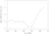 |
Fig. 1. Predicted mass-loss rates (Ṁ) vs Teff for a 60 M⊙ model. |
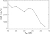 |
Fig. 2. Predicted wind velocity (v∞) vs Teff for a 60 M⊙ model. |
Figure 1 shows that the mass-loss rates increase dramatically by an order of magnitude between 25 000 and 20 000 K. Moreover, the terminal wind velocity is found to drop significantly over the same temperature range (Fig. 2). This second result is new, whilst the first result is more dramatic than the factor of five found from the semi-empirical Vink et al. (1999) models, although the overall mass-loss rates are in reasonable agreement with the Vink et al. (1999, 2000, 2001) rates.
Figure 2 shows relatively low terminal wind velocities on the cool side of the bi-stability jump down to 400 km s−1, instead of values in the range of 2000–3500 km s−1 for hotter objects. As the stellar escape velocity also drops at lower Teff, due to the larger stellar radii, it is more insightful to consider the ratio of v∞ to vesc instead. This ratio is plotted in Fig. 3. It can be seen that the ratio drops rather steeply from values greater than 3 at hot temperatures to values below 1 on the cool side of the bi-stability jump.
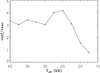 |
Fig. 3. Predicted ratio between the wind velocity (v∞) and the escape velocity (vesc) vs Teff for the 60 M⊙ model. |
We note that observationally Crowther et al. (2006) found somewhat lower values for this ratio with an average value of 3.4 on the hot side of the bi-stability range, and somewhat higher values on the cool side (an average value of 1.9). This raises the question of whether our predicted wind velocities are too high on the hot side of the bi-stability jump and too low on the cool side, which would have consequences for our predicted massloss rates as well. For this reason it is helpful to consider the wind momentum efficiency number η which is defined as the ratio between the wind momentum per unit time (Ṁv∞) over the momentum of the radiation field per unit time (L/c), or η = Ṁv∞/(L/c), and displayed in Fig. 4. Similar to the earlier computations of Vink et al. (2000), the η behaviour shows an increase in the wind efficiency by a factor of 2–3 from 25 000 K onwards, now peaking at 20 000 K. This bi-stability temperature is in agreement with the peak temperature of our alternative CMFGEN approach of Petrov et al. (2016), as well as the observed bi-stability location around spectral type B1 (Lamers et al. 1995; Crowther et al. 2006).
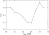 |
Fig. 4. Predicted wind efficiency ratio η vs Teff for the 60 M⊙ model. |
As the mass-loss rate discrepancy is considered to be unresolvable at the current time until appropriate atmosphere modelling including macro-clumping becomes a reality, the issue of the wind terminal velocity deserves extra attention as it is generally considered to be the more robust empirical wind parameter. The velocity values are generally derived from the maximum blue-shifted absorption in resonance lines in the ultraviolet part of the spectrum. Systematic errors may work in both directions, and it may be difficult to see how empirical values could be underestimated on the hot side of the bi-stability jump, whilst being overestimated on the cool side of the jump.
However, it is not inconceivable that this would indeed be the case when the wind physics completely changes at 21 000 K. It is very possible, for instance, that for the faster winds on the hot side of the bi-stability jump the measured lines have not yet reached their predicted terminal wind speeds resulting in an underestimation of v∞, whilst the slower winds on the cool side of the jump may be overestimated due to an increased wind turbulence. This is rather speculative, and would require further investigation to find out whether the outflow speeds on the cool side of the jump are indeed as fast as derived empirically, or as slow as predicted by our Monte Carlo modelling.
A stronger bi-stability jump may have important consequences for bi-stability braking (Vink et al. 2010; Markova et al. 2014; Keszthelyi et al. 2017) and for the formation of dense disks around B[e] supergiants via the rotationally induced bi-stability jump mechanism of Lamers & Pauldrach (1991). The basic idea of this model is that the cooler stellar equator has a higher mass flux and lower wind velocity than the hotter pole, due to the Von Zeipel effect. In the updated computations of Pelupessy et al. (2000) that employed the wind parameters of Vink et al. (1999) this resulted in a density contrast between the equator and the pole of a factor of 10. At the time this was deemed insufficient to explain the dense disks of B[e] supergiants, which lead Curé et al. (2005) to combine the bi-stability mechanism with slow wind solutions at very high rotation speeds.
Our new bi-stability models here predict both an order of magnitude increase in the mass-loss rate and an order of magnitude drop in the wind velocity. In the 2D models of Pelupessy et al. (2000) and Müller & Vink (2014) this implies a density contrast of a factor of 100 between the stellar equator and the pole which may be sufficient to explain the disk density of B[e] supergiants (Kraus 2017). Future multi-dimensional computations are needed in order to determine whether the disk can remain at this high density in the presence of non-radial line forces (Owocki et al. 1996), whilst we also require an explanation for the outflow speeds of just tens of km s−1 (Kraus et al. 2010, 2016; Cidale et al. 2012).
Another interesting puzzle regarding wind velocities in massive stars involves the obscured supergiant HMXB IGR J17252-3616 uncovered by INTEGRAL. Manousakis et al. (2012) performed hydro-dynamical modelling which appears similar to the unobscured classical system Vela X-1, but the authors could only explain the obscured system with a slow wind of the order of 500 km s−1. A possible explanation for the low terminal velocity in IGR J17252-3616 and other HMXBs such as Vela X1 (see Sander et al. 2018) would be that the supergiant donor star might be located on the cool side of the bi-stability jump where the outflow velocity is found to be lower. However, more work is needed to study the ionization and wind physics in the donor stars of HMXBs.
4. Mass loss from luminous blue variables
For the second part of the paper we extend the supergiant computations to models characteristic of LBVs. The defining property of LBVs is their S Doradus variability on timescales of years (Humphreys & Davidson 1994; Vink 2012), which might be explained by stellar radius inflation (Gräfener et al. 2012). This property enables individual stars to cross the bi-stability jump on relatively short evolutionary timescales.
We adopt similar hydrogen (X = 0.38) and helium (Y = 0.60) fractions to those we adopted in Vink & de Koter (2002), and as a representative model set we chose a set of mass, luminosity, and associated Eddington Γ factors similar to those used in that paper. For the first model set in Table 2 we chose a much lower mass (35 M⊙) for the same luminosity of log(L/L⊙) = 6.0, as in the previous section, resulting in an Eddington factor of 0.5, whilst the next series of models were chosen to have masses of 25 and 23 solar masses – for the same fixed luminosity – resulting in Eddington factors of 0.7 and 0.8, respectively. We note that these Eddington Γ values only include the opacity of electron scattering, and for a discussion on the total opacity, we refer the reader to Vink et al. (2011). The relevance of the Eddington parameter for mass-loss rates was highlighted for VMS in the VLT Flames Tarantula Survey (Bestenlehner et al. 2014).
Wind models for a range of three series of LBV models.
The results from Table 2 are plotted in Figs. 5–9, showing the mass-loss rates, wind terminal velocities, ratio of wind velocity to escape velocity, wind structure parameter β, and wind efficiency number η, respectively. The results are qualitatively similar to the earlier 60 M⊙ supergiant model. We note that the jumps for these LBV models are steeper than for the supergiant model, and that in contrast to previous globally consistent predictions in Vink & de Koter (2002) the jump for LBVs has now shifted to the correct effective temperature of approximately 21 000 K. It is thought that the reason for the onset of the bi-stability jump at a lower temperature than previously is that for the stars on the hot side of the jump the winds are now thinner (due to the lower mass-loss rates and higher wind velocities) and that the lower density causes the Fe IV to III recombination of Vink et al. (1999) to occur at a lower effective temperature.
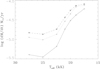 |
Fig. 5. Predicted mass-loss rates (Ṁ) vs Teff for three different mass and Eddington Γ values. The solid line is for M = 35 M⊙, the dotted line for M = 25 M⊙, whilst the dashed line is for M = 23 M⊙, representing Γ values of respectively 0.5, 0.7, and 0.8. |
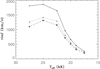 |
Fig. 6. Predicted wind velocity (v∞) vs Teff for the three different LBV mass models. The solid line is for M = 35 M⊙, the dotted line for M = 25 M⊙, whilst the dashed line is for M = 23 M⊙, representing Γ values of respectively 0.5, 0.7, and 0.8. |
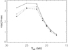 |
Fig. 7. Predicted ratio of the wind velocity (v∞) to the escape velocity (vesc) for the three different LBV mass models. The solid line is for M = 35 M⊙, the dotted line for M = 25 M⊙, whilst the dashed line is for M = 23 M⊙, representing Γ values of respectively 0.5, 0.7, and 0.8. |
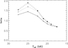 |
Fig. 8. Predicted wind structure parameter βeff for the three different LBV mass models. The solid line is for M = 35 M⊙, the dotted line for M = 25 M⊙, whilst the dashed line is for M = 23 M⊙, representing Γ values of respectively 0.5, 0.7, and 0.8. |
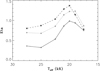 |
Fig. 9. Predicted wind efficiency number η vs Teff for the three different LBV mass models. The solid line is for M = 35 M⊙, the dotted line for M = 25 M⊙, whilst the dashed line is for M = 23 M⊙, representing Γ values of respectively 0.5, 0.7, and 0.8. |
An additional finding is that the size of the bi-stability jump, perhaps unexpectedly, is less pronounced at higher Γ values. We interpret this to be the result of saturation. Higher Γ models already show higher mass-loss rates (and associated lower terminal wind velocities) than lower Γ models on the hot side of the bi-stability jump, so there is less opportunity for a dramatic increase in Ṁ on the cool side of the bi-stability jump.
The absolute values of the terminal wind velocities are now down to 200 km s−1, which is in the correct range for S Doradus type LBVs (Vink 2012). These slow winds are consistent with LBVs being the direct progenitors of Type IIb and IIn supernovae inferred from the the slow outflows (Kotak & Vink 2006; Trundle et al. 2008; Smith et al. 2008; Groh & Vink 2011; Groh 2014; Gräfener & Vink 2016), and inconsistent with the fast outflows expected from Wolf–Rayet stars (Soderberg et al. 2006; Gal-Yam et al. 2014).
The steepest part of the increase in the mass-loss rate is seen in the temperature range 22–20 kK, i.e. at lower values of Teff than suggested in the Vink et al. (2000, 2001) mass-loss recipe. These lower Teff values of the bi-stability agree well with the observed drop in terminal wind velocity around spectral type B1 (Lamers et al. 1995; Crowther et al. 2006) and with CMFGEN modelling by Petrov et al. (2014, 2016). This means that our earlier attribution of the bi-stability jump temperature offset to the use of the modified nebular approximation was not correct. The reason for the discrepancy was the semi-empirical nature of the earlier approach.
Figure 8 shows the behaviour of the wind structure parameter β as a function of temperature. Whilst values on both the cool and the hot side of the bi-stability jump are in the range 0.7–1.5, and are in general agreement with earlier CAK-type models (Pauldrach et al. 1986; Müller & Vink 2008; Muijres et al. 2012, at the bi-stability jump the β parameter peaks at higher values of the order of 1.5–2. We attribute this to several ionization stages of the driving ions playing a role, and in more sophisticated modelling a β law would not be appropriate to describe the dynamical wind behaviour in detail (see e.g. Sander et al. 2018). We note that for models on the cool side of the bi-stability jump below 20 kK the derived β values are no higher than for O star models, i.e. in the range 0.7–1. This contrasts with the high β values of up to 2–3 derived from empirical Hα modelling (Trundle et al. 2004; Crowther et al. 2006), which may be artificially high due to the neglect of optically thick (macro) clumping in the atmosphere modelling (Petrov et al. 2014).
Finally, we note that we did not converge dynamical models at Teff values in the range of the second bi-stability jump around 10 000 K (Lamers et al. 1995; Petrov et al. 2016).
5. Metallicity dependence of the bi-stability jump for LBVs
As a next step in our modelling we vary the metal content Z in order to investigate whether the size of the bi-stability jump is expected to be different in lower Z galaxies, which are also representative of massive stars at earlier Cosmic times. For this purpose we zoom in on the relevant Teff range for the bi-stability jump over a Z range varying from solar, to values as low as 1% solar, with results listed in Table 3 and plotted in Figs. 10 and 11.
Wind models for the same three LBV mass ranges as shown before, but now as a function of Z.
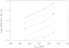 |
Fig. 10. Predicted LBV mass-loss rates ( Ṁ)vs Teff for five metallicities. The solid line is for solar metallicity, whilst the dotted, dashed, dot– dashed, and dot–dot–dot–dashed lines are for 33%, 10%, 3.33%, and 1% solar metallicity, respectively. |
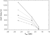 |
Fig. 11. Predicted LBV wind velocities (v∞)vs Teff for five metallicities. The symbols are the same as in Fig. 10. |
As expected, mass-loss rates generally drop with lower Z (Fig. 10), whilst terminal wind velocities display the opposite behaviour with Teff (Fig. 11). At Teff values below the bi-stability jump, terminal velocities seem to converge to similar values for all metallicities (see also Vink 2018). The size of the bi-stability jump indeed appears to be a function of Z, with higher Z giving rise to a larger bi-stability jump, due to an increase in the role of Fe in the line driving at higher Z (Vink et al. 2001).
Kalari et al.(2018) recently investigated the incidence of S Doradus variability amongst normal B supergiants in the low metallicity environment of the Small Magellanic Cloud (SMC), finding a surprisingly low number of S Dor variables in the SMC. This may be related to our finding of lower Z leading to a smaller bi-stability jump.
6. Summary
We presented mass-loss predictions from Monte Carlo radiative transfer models for early-type supergiants and LBVs. Our findings can be summarized as follows:
The previously discovered observed drop in terminal wind velocities at spectral type B1 is confirmed by our dynamically consistent supergiant models;
The bi-stability jump in mass-loss rate is stronger than was derived in previous Monte Carlo modelling;
This would imply that within the rotationally induced bi-stability model of Pelupessy et al. (2000) for B[e] supergiants, the expected density contrast between the hotter pole and cooler equator could increase by up to one order of magnitude – to a factor of 100 – which may be sufficient to account for the disk densities of B[e] supergiants, although the disk velocity structure would still need to be explained;
Our wind predictions may have relevance for the slow wind inferred for the HMXB IGR J17252-3616 or other HMXBs;
The temperature of the bi-stability jump is now at the observed location of 21 000 K, in agreement with CMFGEN models. This boosts confidence in the applicability of the modified nebular approximation;
The bi-stability jump is larger at lower Eddington Γ values; – The bi-stability jump is larger at higher metallicity.
Acknowledgments
I would like to thank the anonymous referee for a constructive report. I acknowledge the hospitality of the Kavli Institute for Theoretical Physics (KITP), Santa Barbara, and thank Ed van den Heuvel for introducing me to the problem of the slow wind in IGR J17252-3616 during my stay at KITP, which was supported by the National Science Foundation under Grant No. NSF PHY11-25915.
References
- Abbott, D. C., & Lucy, L. B. 1985, ApJ, 288, 679 [NASA ADS] [CrossRef] [Google Scholar]
- Anders, E., & Grevesse, N. 1989, GeCoA, 53, 197 [Google Scholar]
- Benaglia, P., Vink, J. S., Martí, J., et al. 2007, A&A, 467, 1265 [NASA ADS] [CrossRef] [EDP Sciences] [Google Scholar]
- Bestenlehner, J. M., Gräfener, G., Vink, J. S., et al. 2014, A&A, 570, A38 [NASA ADS] [CrossRef] [EDP Sciences] [Google Scholar]
- Castor, J., Abbott, D. C., & Klein, R. I. 1975, ApJ, 195, 157 [NASA ADS] [CrossRef] [Google Scholar]
- Chiosi, C., & Maeder, A. 1986, ARA&A, 24, 329 [NASA ADS] [CrossRef] [Google Scholar]
- Cidale, L. S., Borges Fernandes, M., Andruchow, I., et al. 2012, A&A, 548, A72 [NASA ADS] [CrossRef] [EDP Sciences] [Google Scholar]
- Crowther, P. A., Lennon, D. J., & Walborn, N. R. 2006, A&A, 446, 279 [NASA ADS] [CrossRef] [EDP Sciences] [Google Scholar]
- Curé, M., Rial, D. F., & Cidale, L. 2005, A&A, 437, 929 [NASA ADS] [CrossRef] [EDP Sciences] [Google Scholar]
- Davies, B., Vink, J. S., & Oudmaijer, R. D. 2007, A&A, 469, 1045 [NASA ADS] [CrossRef] [EDP Sciences] [Google Scholar]
- de Koter, A., Schmutz, W., & Lamers, H. J. G. L. M. 1993, A&A, 277, 561 [NASA ADS] [Google Scholar]
- Gal-Yam, A., Arcavi, I., Ofek, E. O., et al. 2014, Nature, 509, 471 [NASA ADS] [CrossRef] [Google Scholar]
- Gräfener, G., & Vink, J. S. 2016, MNRAS, 455, 112 [NASA ADS] [CrossRef] [Google Scholar]
- Gräfener, G., Owocki, S. P., & Vink, J. S. 2012, A&A, 538, A40 [NASA ADS] [CrossRef] [EDP Sciences] [Google Scholar]
- Groh, J. H. 2014, A&A, 572, L11 [NASA ADS] [CrossRef] [EDP Sciences] [Google Scholar]
- Groh, J. H., & Vink, J. S. 2011, A&A, 531, L10 [NASA ADS] [CrossRef] [EDP Sciences] [Google Scholar]
- Groh, J. H., Meynet, G., Ekström, S., & Georgy, C. 2014, A&A, 564, A30 [NASA ADS] [CrossRef] [EDP Sciences] [Google Scholar]
- Hamann, W.-R., Feldmeier, A., & Oskinova, L. M. 2008, Clumping in Hot-Star Winds [Google Scholar]
- Hillier, D. J. 1991, A&A, 247, 455 [NASA ADS] [Google Scholar]
- Humphreys, R. M., & Davidson, K. 1994, PASP, 106, 1025 [NASA ADS] [CrossRef] [Google Scholar]
- Jiang, Y.-F., Cantiello, M., Bildsten, L., Quataert, E., & Blaes, O. 2015, ApJ, 813, 74 [NASA ADS] [CrossRef] [Google Scholar]
- Kalari, V. M., Vink, J. S., Dufton, P. L., & Fraser, M. 2018, A&A, 618, A17 [NASA ADS] [CrossRef] [EDP Sciences] [Google Scholar]
- Keszthelyi, Z., Puls, J., & Wade, G. A. 2017, A&A, 598, A4 [NASA ADS] [CrossRef] [EDP Sciences] [Google Scholar]
- Kotak, R., & Vink, J. S. 2006, A&A, 460, L5 [NASA ADS] [CrossRef] [EDP Sciences] [Google Scholar]
- Kraus, M. 2017, The B[e] Phenomenon: Forty Years of Studies, 508, 219 [NASA ADS] [Google Scholar]
- Kraus, M., Borges Fernandes, M., & de Araújo, F. X. 2010, A&A, 517, A30 [NASA ADS] [CrossRef] [EDP Sciences] [Google Scholar]
- Kraus, M., Cidale, L. S., Arias, M. L., et al. 2016, A&A, 593, A112 [NASA ADS] [CrossRef] [EDP Sciences] [Google Scholar]
- Krtička, J., & Kubát, J. 2017, A&A, 606, A31 [NASA ADS] [CrossRef] [EDP Sciences] [Google Scholar]
- Kurucz, R. L., & Bell, B. 1995, Atomic Line Data Kurucz CD-ROM No. 23 (Cambridge, MA: Smithsonian Astrophysical Observatory) [Google Scholar]
- Lamers, H. J. G. L. M., & Pauldrach, A. W. A. 1991, A&A, 244, L5 [NASA ADS] [Google Scholar]
- Lamers, H. J. G. L. M., Snow, T. P., & Lindholm, D. M. 1995, ApJ, 455, 269 [NASA ADS] [CrossRef] [Google Scholar]
- Langer, N. 2012, ARA&A, 50, 107 [NASA ADS] [CrossRef] [Google Scholar]
- Lucy, L. B., & Solomon, P. M. 1970, ApJ, 159, 879 [NASA ADS] [CrossRef] [Google Scholar]
- Manousakis, A., Walter, R., & Blondin, J. M. 2012, A&A, 547, A20 [NASA ADS] [CrossRef] [EDP Sciences] [Google Scholar]
- Markova, N., & Puls, J. 2008, A&A, 478, 823 [NASA ADS] [CrossRef] [EDP Sciences] [Google Scholar]
- Markova, N., Puls, J., Simón-Díaz, S., et al. 2014, A&A, 562, A37 [NASA ADS] [CrossRef] [EDP Sciences] [Google Scholar]
- Moffat, A. F. J., & Robert, C. 1994, ApJ, 421, 310 [NASA ADS] [CrossRef] [Google Scholar]
- Morford, J. C., Fenech, D. M., Prinja, R. K., Blomme, R., & Yates, J. A. 2016, MNRAS, 463, 763 [NASA ADS] [CrossRef] [Google Scholar]
- Muijres, L. E., de Koter, A., Vink, J. S., et al. 2011, A&A, 526, A32 [Google Scholar]
- Muijres, L. E., Vink, J. S., de Koter, A., Müller, P. E., & Langer, N. 2012, A&A, 537, A37 [NASA ADS] [CrossRef] [EDP Sciences] [Google Scholar]
- Müller, P. E., & Vink, J. S. 2008, A&A, 492, 493 [NASA ADS] [CrossRef] [EDP Sciences] [Google Scholar]
- Müller, P. E., & Vink, J. S. 2014, A&A, 564, A57 [NASA ADS] [CrossRef] [EDP Sciences] [Google Scholar]
- Oskinova, L. M., Hamann, W.-R., & Feldmeier, A. 2007, A&A, 476, 1331 [NASA ADS] [CrossRef] [EDP Sciences] [Google Scholar]
- Owocki, S. P. 2015, Very Massive Stars in the Local Universe, 412, 113 [NASA ADS] [CrossRef] [Google Scholar]
- Owocki, S. P., Cranmer, S. R., & Gayley, K. G. 1996, ApJ, 472, L115 [NASA ADS] [CrossRef] [Google Scholar]
- Pauldrach, A. W. A., & Puls, J. 1990, A&A, 237, 409 [NASA ADS] [Google Scholar]
- Pauldrach, A. W. A., Puls, J., & Kudritzki, R. P. 1986, A&A, 164, 86 [Google Scholar]
- Pelupessy, I., Lamers, H. J. G. L. M., & Vink, J. S. 2000, A&A, 359, 695 [NASA ADS] [Google Scholar]
- Petrov, B., Vink, J. S., & Gräfener, G. 2014, A&A, 565, A62 [NASA ADS] [CrossRef] [EDP Sciences] [Google Scholar]
- Petrov, B., Vink, J. S., & Gräfener, G. 2016, MNRAS, 458, 1999 [NASA ADS] [CrossRef] [Google Scholar]
- Puls, J., Vink, J. S., & Najarro, F. 2008, A&ARv, 16, 209 [NASA ADS] [CrossRef] [EDP Sciences] [Google Scholar]
- Ramírez-Agudelo, O. H., Sana, H., de Koter, A., et al. 2017, A&A, 600, A81 [NASA ADS] [CrossRef] [EDP Sciences] [Google Scholar]
- Sander, A. A. C., Fürst, F., Kretschmar, P., et al. 2018, A&A, 610, A60 [Google Scholar]
- Shaviv, N. J. 2000, ApJ, 532, L137 [NASA ADS] [CrossRef] [PubMed] [Google Scholar]
- Smith, N., & Owocki, S. P. 2006, ApJ, 645, L45 [NASA ADS] [CrossRef] [Google Scholar]
- Smith, N., Chornock, R., Li, W., et al. 2008, ApJ, 686, 467 [NASA ADS] [CrossRef] [Google Scholar]
- Schmutz, W. 1991, in Stellar Atmospheres: Beyond Classical Models, eds. L. Crivellari, I. Hubeny, & D. G. Hummer, NATO ASI Ser. C, 341, 191 [Google Scholar]
- Soderberg, A. M., Chevalier, R. A., Kulkarni, S. R., & Frail, D. A. 2006, ApJ, 651, 1005 [NASA ADS] [CrossRef] [Google Scholar]
- Sundqvist, J. O., Puls, J., & Owocki, S. P. 2014, A&A, 568, A59 [NASA ADS] [CrossRef] [EDP Sciences] [Google Scholar]
- Šurlan, B., Hamann, W.-R., Aret, A., et al. 2013, A&A, 559, A130 [NASA ADS] [CrossRef] [EDP Sciences] [Google Scholar]
- Trundle, C., Lennon, D. J., Puls, J., & Dufton, P. L. 2004, A&A, 417, 217 [NASA ADS] [CrossRef] [EDP Sciences] [Google Scholar]
- Trundle, C., Kotak, R., Vink, J. S., & Meikle, W. P. S. 2008, A&A, 483, L47 [NASA ADS] [CrossRef] [EDP Sciences] [Google Scholar]
- van Marle, A. J., Owocki, S. P., & Shaviv, N. J. 2008, MNRAS, 389, 1353 [NASA ADS] [CrossRef] [Google Scholar]
- Vink, J. S. 2012, Eta Carinae and the Supernova Impostors, 384, 221 [Google Scholar]
- Vink, J. S. 2018, A&A, 615, A119 [NASA ADS] [CrossRef] [EDP Sciences] [Google Scholar]
- Vink, J. S., & de Koter, A. 2002, A&A, 393, 543 [NASA ADS] [CrossRef] [EDP Sciences] [Google Scholar]
- Vink, J. S., & Gräfener, G. 2012, ApJ, 751, L34 [NASA ADS] [CrossRef] [Google Scholar]
- Vink, J. S., de Koter, A., & Lamers, H. J. G. L. M. 1999, A&A, 345, 109 [Google Scholar]
- Vink, J. S., de Koter, A., & Lamers, H. J. G. L. M. 2000, A&A, 362, 295 [NASA ADS] [Google Scholar]
- Vink, J. S., de Koter, A., & Lamers, H. J. G. L. M. 2001, A&A, 369, 574 [NASA ADS] [CrossRef] [EDP Sciences] [Google Scholar]
- Vink, J. S., Brott, I., Gräfener, G., et al. 2010, A&A, 512, L7 [NASA ADS] [CrossRef] [EDP Sciences] [Google Scholar]
- Vink, J. S., Muijres, L. E., Anthonisse, B., et al. 2011, A&A, 531, A132 [NASA ADS] [CrossRef] [EDP Sciences] [Google Scholar]
All Tables
Wind predictions for a 60 M⊙ model with stellar parameters identical to model series #10 from Vink et al. (2000).
Wind models for the same three LBV mass ranges as shown before, but now as a function of Z.
All Figures
|
Fig. 1. Predicted mass-loss rates (Ṁ) vs Teff for a 60 M⊙ model. |
| In the text | |
|
Fig. 2. Predicted wind velocity (v∞) vs Teff for a 60 M⊙ model. |
| In the text | |
|
Fig. 3. Predicted ratio between the wind velocity (v∞) and the escape velocity (vesc) vs Teff for the 60 M⊙ model. |
| In the text | |
|
Fig. 4. Predicted wind efficiency ratio η vs Teff for the 60 M⊙ model. |
| In the text | |
|
Fig. 5. Predicted mass-loss rates (Ṁ) vs Teff for three different mass and Eddington Γ values. The solid line is for M = 35 M⊙, the dotted line for M = 25 M⊙, whilst the dashed line is for M = 23 M⊙, representing Γ values of respectively 0.5, 0.7, and 0.8. |
| In the text | |
|
Fig. 6. Predicted wind velocity (v∞) vs Teff for the three different LBV mass models. The solid line is for M = 35 M⊙, the dotted line for M = 25 M⊙, whilst the dashed line is for M = 23 M⊙, representing Γ values of respectively 0.5, 0.7, and 0.8. |
| In the text | |
|
Fig. 7. Predicted ratio of the wind velocity (v∞) to the escape velocity (vesc) for the three different LBV mass models. The solid line is for M = 35 M⊙, the dotted line for M = 25 M⊙, whilst the dashed line is for M = 23 M⊙, representing Γ values of respectively 0.5, 0.7, and 0.8. |
| In the text | |
|
Fig. 8. Predicted wind structure parameter βeff for the three different LBV mass models. The solid line is for M = 35 M⊙, the dotted line for M = 25 M⊙, whilst the dashed line is for M = 23 M⊙, representing Γ values of respectively 0.5, 0.7, and 0.8. |
| In the text | |
|
Fig. 9. Predicted wind efficiency number η vs Teff for the three different LBV mass models. The solid line is for M = 35 M⊙, the dotted line for M = 25 M⊙, whilst the dashed line is for M = 23 M⊙, representing Γ values of respectively 0.5, 0.7, and 0.8. |
| In the text | |
|
Fig. 10. Predicted LBV mass-loss rates ( Ṁ)vs Teff for five metallicities. The solid line is for solar metallicity, whilst the dotted, dashed, dot– dashed, and dot–dot–dot–dashed lines are for 33%, 10%, 3.33%, and 1% solar metallicity, respectively. |
| In the text | |
|
Fig. 11. Predicted LBV wind velocities (v∞)vs Teff for five metallicities. The symbols are the same as in Fig. 10. |
| In the text | |
Current usage metrics show cumulative count of Article Views (full-text article views including HTML views, PDF and ePub downloads, according to the available data) and Abstracts Views on Vision4Press platform.
Data correspond to usage on the plateform after 2015. The current usage metrics is available 48-96 hours after online publication and is updated daily on week days.
Initial download of the metrics may take a while.