| Issue |
A&A
Volume 619, November 2018
|
|
|---|---|---|
| Article Number | A75 | |
| Number of page(s) | 6 | |
| Section | Extragalactic astronomy | |
| DOI | https://doi.org/10.1051/0004-6361/201833332 | |
| Published online | 09 November 2018 | |
Focusing on the extended X-ray emission in 3C 459 with a Chandra follow-up observation
1
Dipartimento di Fisica, Universitydegli Studi di Cagliari, Complesso Universitario di Monserrato, S. P. Monserrato-Sestukm 0.700, 09042 Monserrato CA, Italy
e-mail: This email address is being protected from spambots. You need JavaScript enabled to view it.
2
Harvard – Smithsonian Astrophysical Observatory, Cambridge, MA 02138, USA
3
Dipartimento di Fisica, University degli Studi di Torino. via Pietro Giuria 1, 10125 Torino, Italy
4
Istituto Nazionale di Fisica Nucleare, Sezione di Torino, 10125, Torino, Italy
5
Istituto Nazionale di Astrofisica, Sezione di Torino, 10125 Torino, Italy
6
Consorzio Interuniversitario per la Fisica Spaziale (CIFS), via Pietro Giuria 1, 10125 Torino, Italy
7
School of Physics, Astronomy and Mathematics, University of Hertfordshire, College Lane, Hatfield AL10 9AB, UK
Received:
1
May
2018
Accepted:
25
August
2018
Abstract
Aims. We investigated the X-ray emission properties of the powerful radio galaxy 3C 459 revealed by a recent Chandra follow-up observation carried out in October 2014 with a 62 ks exposure.
Methods. We performed an X-ray spectral analysis from a few selected regions on an image obtained from this observation and also compared the X-ray image with a 4.9 GHz VLA radio map available in the literature.
Results. The dominant contribution comes from the radio core but significant X-ray emission is detected at larger angular separations from it, surrounding both radio jets and lobes. According to a scenario in which the extended X-ray emission is due to a plasma collisionally heated by jet-driven shocks and not magnetically dominated, we estimated its temperature to be ∼0.8 keV. This hot gas cocoon could be responsible for the radio depolarization observed in 3C 459, as recently proposed also for 3C 171 and 3C 305. On the other hand, our spectral analysis and the presence of an oxygen K edge, blueshifted at 1.23 keV, cannot exclude the possibility that the X-ray radiation originating from the inner regions of the radio galaxy could be intercepted by some outflow of absorbing material intervening along the line of sight, as already found in some BAL quasars.
Key words: galaxies: active / galaxies: clusters: individual: 3C 459 / radio continuum / galaxies: X-rays: general
© ESO 2018
1. Introduction
Recent developments in both theory and observations have highlighted the role of feedback from radio-loud active galactic nuclei (AGNs) in the evolution of galaxies (e.g., Silk & Rees 1998; Di Matteo et al. 2005; Morganti et al. 2013). The interaction between radio jets and the interstellar medium (ISM) inhibits the growth of the supermassive black hole and affects the star formation rate. Jets drive large-scale outflows of neutral (e.g., Morganti et al. 2003) and ionized (e.g., Crenshaw et al. 2003) gas, which strips away raw materials needed for star formation. Moreover, jets would induce turbulence and shocks into the ISM creating less favorable conditions for the formation of new stars (Wagner & Bicknell 2011). A considerable amount of gas surrounding jets and lobes, heated and ionized by shocks in the ISM, is also responsible for the depolarization observed at radio frequencies (e.g., Heckman et al. 1982; Hardcastle 2003). This hot and ionized gas is often associated with the extended emission line regions (EELR) detected in the optical band and generally aligned with radio jets (e.g., McCarthy et al. 1996); deviations from such an alignment were found in radio galaxies at z < 0.5 extending for more than 150 kpc whose emitting line regions show a filamentary structure extending for a few tens of kiloparsecs (Baum & Heckman 1989).
According to this picture, jets are therefore an efficient mechanism to convert the energy output from the AGN core into an energy input into the ISM (Guillard et al. 2012). However, detailed descriptions of the shock’s behavior have only been performed for a limited number of nearby sources to date (see, e.g., the analysis carried out by Kraft et al. (2003) for Centaurus A). Therefore, the details of this jet-ISM interaction are not yet firmly established. Multifrequency observations of nearby active galaxies are the key to shedding light on this process.
Important contributions have recently come from X-ray observations. During Chandra Cycle 9 a snapshot survey was started to complete the multifrequency database of the revised Third Cambridge catalog (3CR) with X-ray observations (Massaro et al. 2010, 2012, 2013). In addition, recent observations were carried out with the Swift satellite to increase the completeness of the sample (Maselli et al. 2016). All 3CR radio sources with z ≤ 1.5 have at least an X-ray snapshot observation present in the Chandra archive to date (Massaro et al. 2015, 2018; Stuardi et al. 2018). This X-ray database is also enriched by observations that have comparable angular resolution and performed in the radio, infrared, and optical bands (see, e.g., Werner et al. 2012; Dicken et al. 2014; Buttiglione et al. 2009, 2011; Madrid et al. 2006; Privon et al. 2008; Tremblay et al. 2009; Hilbert et al. 2016).
The Chandra snapshot survey of 3CR sources at low red-shift (Massaro et al. 2010) was also used to plan follow-up observations of selected targets showing extended X-ray emission (Massaro et al. 2012) or with peculiar features, as is the case for 3C 305 (Massaro et al. 2009; Hardcastle et al. 2012) and 3C 171 (Hardcastle et al. 2010). This is also the case for 3C 459, for which we present here the results of our Chandra follow-up observation.
A brief summary of the multifrequency properties of 3C 459 is presented in Sect. 2, while details of the X-ray data reduction are reported in Sect. 3. The analysis is then presented in Sect. 4, with Sect. 5 finally devoted to the discussion of our results and conclusions.
We assume hereafter a flat cosmology with H0 = 72 km s−1, Mpc−1, ΩM = 0.26, and ΩΛ = 0.74 (Dunkley et al. 2009). 3C 459 lies at z = 0.22 (Holt et al. 2008) where 1 arcsec corresponds to 3.476 kpc and its luminosity distance is 1067.2 Mpc (Wright 2006).
2. The peculiar radio galaxy 3C 459
Source 3C 459 is a powerful radio galaxy included in the revised Third Cambridge Catalog (Spinrad et al. 1985) as well as in the 2 Jy sample (Wall & Peacock 1985). The first detailed radio morphological analysis on this source, carried out by Ulvestad (1985), showed a steep-spectrum core and two edge-brightened lobes with an evident asymmetric profile, for a total extension of 8.2″ (i.e., 28.5 kpc). The angular separation between the western lobe and the core is about five times larger than that from the eastern one (1.3″). On the basis of its radio morphology, 3C 459 has also been classified as a compact steep-spectrum (CSS) source (see, e.g., Gelderman & Whittle 1994; see also O’Dea 1998 for a review on these objects) though it is not included in the CSS sample originally assembled by Spencer et al. (1989). Thomasson et al. (2003) presented a very long baseline interferometry (VLBI) image of the central core showing a complex structure consistent with a strongly bent jet, attributed to the impact of the eastern jet with a large amount of gas in the ISM. The eastern lobe appears to be significantly depolarized while the western lobe is not. This source is thus characterized by a high degree of asymmetry in both its morphology and depolarization (Ulvestad 1985; Morganti et al. 1999; Thomasson et al. 2003). Evidence of fast and massive outflows of neutral gas was also reported by Morganti et al. (2005); Guillard et al. (2012) confirmed this result and traced the presence of ionized gas.
Source 3C 459 has also been intensively observed at higher frequencies. In the far-infrared, it is about an order of magnitude brighter than other objects in the 2 Jy sample at similar redshift (Tadhunter et al. 2002; Dicken et al. 2009).
Miller (1981) first published an optical-ultraviolet (UV) spectrum and noticed the presence of the Balmer break and higher Balmer absorption lines. This was interpreted as due to photospheres of A-type stars rather than ISM (Tadhunter et al. 1996), an interpretation that was later found to be in agreement with spectral synthesis modeling (Wills et al. 2008). The detection in this spectrum of several emission lines, with no clear evidence of broad permitted lines, led Heckman et al. (1994) to classify 3C 459 as a narrow-line radio galaxy.
In Jackson & Rawlings (1997), 3C 459 was also classified as a high excitation radio galaxy (HERG; see, e.g., Best & Heckman 2012) from the analysis of the optical spectrum published by Eracleous & Halpern (1994). This classification was confirmed by Buttiglione et al. (2010) by computing the value of the excitation index (EI), a spectroscopic indicator that measures the relative intensity of low and high excitation lines, using the spectrum published in Buttiglione et al. (2009). In addition, due to the broad shape of the Ha line in this spectrum, Buttiglione et al. (2010) marked 3C 459 as a broad line object (BLO). In their search for extended soft X-ray emission in HERG and BLO, Balmaverde et al. (2012) reported 3C 459 as one of 2 galaxies, among 18 BLOs, showing evidence of such emission and suggested a need for further investigation.
The host galaxy of 3C 459 shows a disturbed optical morphology, with two broad symmetrical fan-like protrusions dominated by continuum emission and extending to the east and the south (Heckman et al. 1986; Ramos Almeida et al. 2011).
The information so far collected in the literature for this source is consistent with a model in which a gas-rich merger episode heated gas and triggered starburst activity (see Wills etal. 2008; Tadhunter et al. 2011). Subsequently, following the coalescence of the nuclei of the merging galaxies, the observed radio jets and the overall AGN activity were also triggered. Thomasson et al. (2003) suggested that the denser gas, responsible for the bending of the eastern jet, could be the result of this merging process.
3. X-ray data reduction
The ∼62 ks follow-up observation presented here (ObsID 16044) was performed on October 12, 2014, with the Chandra ACIS-S camera operating in VERY FAINT mode. The data reduction was carried out following the standard procedures described in the Chandra Interactive Analysis of Observations (CIAO) threads1, and adopted in other analyses (see, e.g., Massaro et al. 2018). We used the CIAO software package version 4.8 and the Chandra Calibration Database (CALDB) version 4.7.2 to process all files. Level 2 event files were generated using the ACIS PROCESS EVENTS task, after removing the hot pixels with ACIS RUN HOTPIX. Events were filtered for grades 0, 2, 3, 4, 6 and pixel randomization was removed. Astrometric registration was carried out by changing the appropriate keywords in the fits header so that the nuclear X-ray position was aligned with the radio one. The 0.5-7.0 keV count map that we obtained following this procedure is shown in the left panel of Fig. 1. The same map, although with a different pixel size, is shown in the right panel of Fig. 2 emphasizing the different energy of the detected counts. For this purpose we distinguished soft (0.5–1.0keV), medium (1.0–2.0 keV), and hard (2.0–7.0 keV) energy bands.
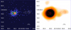 |
Fig. 1. Left panel: unsmoothed map of the Chandra count rate in the 0.5–7.0 keV band, each pixel corresponding to 0.246″, that is half the native Chandra pixel size. The radio contours from a VLA map in the C band have been overlaid (white line): they start at 0.48 mJy beam−1 and stop at 0.24 Jy beam−1 in correspondence of the core. Right panel: Chandra flux map in the same energy band: a circle with a radius of 2″ is centered at the coordinates of the core. |
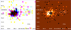 |
Fig. 2. Left panel: composite RGB image of the X-ray count map of 3C 459. The native pixel size, corresponding to 0.492 arcsec, is shown. Different colors distinguish three energy bands: cyan (0.5–1.0 keV), magenta (1.0–2.0 keV), and yellow (2.0–7.0 keV). The contours of adopted extraction regions as described in Sect. 4.1 are marked with black dashed lines. Right panel: map of the hardness ratio obtained adopting 0.5–2.0 keV and 2.0–7.0 keV as the soft (white points) and the hard (black points) X-ray bands, respectively. A smoothing with a Gaussian (σ = 0.123″) has been applied. |
These same bands were used to create flux maps; a global map in the 0.5–7.0 keV energy range, shown in the right panel of Fig. 1, was also built. Flux maps were corrected for exposure time and effective area, and our implementation used monochromatic exposure maps. We fixed the values for the nominal energies assigned to the soft, medium, and hard bands to 0.8, 1.4, and 4 keV, respectively; the exposure maps were built for these nominal values. Since the natural units of X-ray flux maps are counts in cm−2 s−1, we converted them to cgs units by multiplying each event by the nominal energy of its band, thereby assuming that each event in the band has the same energy. Subsequently, when performing photometry, we applied the correction factor required to recover the observed units of erg cm−2 s−1. The “nominal energy” was used only to obtain the correct units. The total energy for any particular region was recovered by applying a correction factor of E(average)/E(nominal) to the photometric measurement. To derive E(average), the actual values were measured with the CIAO tool DMSTAT. This correction typically ranged from a few percent to 15%. A hardness ratio map in the soft (0.5–2.0 keV) and hard (2.0–7.0 keV) X-ray bands (see Fig. 2) was also constructed.
We extracted spectra in the 0.5–7.0 keV energy range using the CIAO SPECEXTRACT script for a few selected regions (see Sect. 4 for details). All spectra were binned to obtain a minimum number of 20 counts per bin after background subtraction, and were analyzed with XSPEC 12. Uncertainties are reported with a 90% level of confidence.
4. X-ray data analysis
4.1. Imaging analysis
To carry out the X-ray analysis we selected three regions as described immediately below and shown in Fig. 2 (left panel). These were chosen by overlaying 4.9 GHz radio contours on to the X-ray image as described in Sect. 3.
A circle C with a radius of 2″, centered at the coordinates used for the astrometric registration and matching the core;
a rectangle W of size 3.44″ × 1.48″ (21 pixels) matching both the western jet and lobe;
a wider rectangle D of size 11.80″ × 6.40″ (312 pixels) encompassing the whole radio structure.
The angular separation between a point along the lowest radio contour and the nearest point on the D perimeter is in the 1.3″–3.5″ range. The region resulting from the difference between D and C (hereinafter labeled as D–C) was used to study the extended X-ray emission only.
The detection significance of the X-ray emission within C, W, and D–C was evaluated comparing their surface brightness (number of X-ray counts per unit area) with that computed in a 50″ radius circle B, centered at 90″ east of the core and lacking any clear X-ray emission due to background sources. In the 0.5–7.0 keV band the surface brightness in C, W, and D–C is (47.8 ± 1.9), (1.2 ± 0.5), and (1.1 ± 0.1) ct arcsec−2, respectively. The values computed in W and D–C, which are very similar to each other, are more than an order of magnitude higher than in B, thus resulting in a significant detection. All details corresponding to this and other energy ranges are reported in Table 1.
Number of counts, and the corresponding surface brightness (counts · arcsec−2), computed in different energy bands within a 2″ radius circle C matching the radio core, a rectangle W matching the western radio jet and lobe, the D–C region matching the extended emission, and a 50″ radius circle B taking into account the background contribution.
4.2. Spectral analysis
For the spectral analysis we assumed that the X-ray emission from 3C 459 has two main components: the former related to its radio core and the latter arising from extended emission. We first describe the analysis of the spectrum extracted from C, where both components are present, and then consider the D spectrum. All models adopted in our analysis include Galactic absorption with column density NH = 5.24 × 1020 cm−2 (Kalberla et al. 2005).
4.2.1. X-ray spectrum extracted from C
The fit of the X-ray spectrum from C with a single unabsorbed power law model was not acceptable (i.e., χ2 of 68.33 for 26 d.o.f.). Fitting with a single, intrinsically absorbed power law did not lead to any significant improvements. In both cases we found clear evidence of a soft excess below 1 keV, as shown in Fig. 3). A fitting procedure with both components improved the χ2 (i.e., 26.47/23 d.o.f.), but led to a high value of the photon index  for the unabsorbed power law. We found
  cm−2 and
  for the absorbed component: the ΓA value, though poorly constrained, is consistent within the errors with ⟨Γ⟩ = 1.7 computed considering most radio-loud AGNs (see, e.g., Hardcastle et al. 2006).
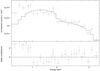 |
Fig. 3. Fit to the X-ray spectrum of 3C 459 (and corresponding residuals) extracted from C in the 0.5–7.0 keV band adopting a single, intrinsically absorbed, power law; a soft excess at energies lower than 1 keV is evident. |
To test the hypothesis that the origin of the soft excess is due to collitionally ionized plasma, we fitted the spectrum with a model including both an Astrophysical Plasma Emission Code (APEC) and an intrinsically absorbed power law. Leaving all parameters free to vary we obtained a good description of the spectrum (χ2 = 22.32, 22 d.o.f.) but some parameter values were poorly constrained: in particular, no improvement was obtained for  while the abundance of elements in the plasma with respect to solar values was equal to 0.07, and consistent with zero. However, such subsolar abundances have already been found in similar spectral analysis carried out for 3C 171 (Hardcastle et al. 2010) and 3C 305 (Hardcastle et al. 2012). Subsequently, we fixed ΓA = 1.7 and the abundance to 0.15 solar, a value that is in line with the results obtained by Hardcastle et al. (2012; see their Table 3). In this way we obtained a plasma temperature
  keV and a hydrogen column density
  cm−2 (χ2 = 25.23, 24 d.o.f.); this fit and the corresponding residuals are shown in the left panel of Fig. 4.
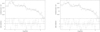 |
Fig. 4. Left panel: fit to the X-ray spectrum of 3C 459 (and corresponding residuals) extracted from C in the 0.5–7.0 keV band with a model including both the APEC and the absorbed power law. Right panel: fit to the same spectrum using an ABSORI component. |
In light of the distribution of residuals shown in Fig. 3, we decided to replace the ZWABS component in our fitting model with ZEDGE, a redshifted absorption edge. This component could be interpreted as due to the presence of an absorbing material intercepting a relativistic outflow along the line of sight. As a result, we obtained an acceptable fit (χ2 = 27.47, 24 d.o.f.) with the absorption edge at energy  keV and the photon index at
  . We further replaced an absorption component from ionized material (i.e., ABSORI) with that arising from a neutral absorber (i.e., ZEDGE). Following this fitting procedure we found indications of high values for both the temperature T abs of the absorbing material and the ionization parameter Freezing them at Tabs = 106 K and ξ = 100, respectively, the fit improves for increasing values of the Fe abundance. Fixing also this last parameter to twice the Solar value, we found χ2 = 25.25 (25 d.o.f.), with NH = (5.7 ± 1.3) × 1022 cm−2 and
  . Results of this fit are shown in the right panel of Fig. 4.
Finally, we also tested a photoionization scenario to describe the ISM thermal emission adding up to three emission lines with a Gaussian profile, with σ at the value of 10−3 keV, to the simple power-law component. Following this procedure, the best result in terms of χ2 (19.25 with 22 d.o.f.) was obtained including two emission lines at energies corresponding to the transitions of heavily photoionized elements (Fe XVII and Ne X). However, the value of the photon index was extremely low (ΓU = 0.89 ± 0.15).
4.2.2. X-ray spectrum extracted from D
Assuming the (APEC + absorbed power law) description for the C region, we fitted the X-ray spectrum extracted from the D region with a similar model but fixing the ΓA ≡ 1.7 and NH to the value that we obtained from the fit of the C spectrum. As a result, we found a reliable description of the spectrum (χ2 = 28.08 with 26 d.o.f.) with the same low value for the abundance as in the C case, but better constrained  , and a lower value of the plasma temperature
  keV; the APEC normalization was
  cm−5.
cm−5.
5. Discussion and conclusions
Here we present results of an X-ray analysis of the follow-up Chandra observation of 3C 459 performed in October 2014 for a total of 62 ks exposure time. Our analysis was carried out selecting several regions, as described in Sect. 4. In particular, the C region takes into account the X-ray emission mainly from the radio core; any eventual contribution from the eastern lobe could not be disentangled from the core emission due to the small angular separation (1.3″) between them. The D–C region takes into account the extended emission surrounding the whole radio galaxy: ∼11% of all the counts detected in D correspond to D–C. In this region, the X-ray emission follows the direction traced by the radio jets, as more clearly visible for the western one (right panel of Fig. 1). The distribution of the X-ray photons is not confined within the lowest radio flux density contour, suggesting that they could come from a plasma that almost uniformly wraps around the whole radio structure.
In recent years, significant efforts have been made to investigate the X-ray emission of compact radio galaxies such as CSS and Gigahertz Peaked Spectrum (GPS; O’Dea et al. 2006; Guainazzi et al. 2006; Vink et al. 2006; Siemiginowska et al. 2008, 2016; Tengstrand et al. 2009; Kunert-Bajraszewska et al. 2014), and are still ongoing. Examining the results from a sample of nine bona fide CSS radio galaxies detected until then in the X rays, O’Dea etal. (2017) found convincing evidence for hot shocked gas for just two of them (3C 303.1 and 3C 305). However, they noticed that both were not exceptional in their overall properties, compared to the total sample ofnine. This led them to speculate that hot shocked gas is typical in CSS sources and would be revealed by performing deeper observations; in this sense, our results on 3C 459 validate this hypothesis.
In line with a scenario where the extended X-ray emission is due to a plasma collisionally heated by jet-driven shocks, we estimated a temperature of 0.78 keV with subsolar abundances. Assuming a cylindrical geometry with r = 3.2″ and h = 11.8″ for the plasma distribution, which is a three-dimensional equivalent of the D rectangle, from the APEC normalization we derived a hydrogen density nH = 5.2 × 10⁻² cm−3. Under the simple assumption that this plasma is not magnetically dominated, implying that the energy density in the magnetic field B2/2μ0 is lower than the thermal energy density in the gas (3/2) nkT, this value provides an upper limit for the magnetic field strength that is B < 55 μG, in agreement with the results already found for other 3C sources observed with Chandra such as 3C 171 (Hardcastle et al. 2010) and 3C 305 (Hardcastle et al. 2012). The assumption that the gas is not magnetically dominated is supported by the fact that radio lobes tend to be close to the equipartition and the magnetic field B is of the order of a few μG (see, e.g., Croston et al. 2005; Duffy & Blundell 2012). Typical B values in radio lobes are similar to BCMB, the magnetic field having equivalent energy density to the cosmic microwave background (CMB) at the source redshift (Massaro & Ajello 2011). For 3C 459 , BCMB is ≈ 5 μG, and therefore has an energy density about one order of magnitude lower than the thermal one.
This hot gas cocoon could be responsible for the radio depolarization observed in 3C 459. Therefore, excluding the contribution from the radio core, whose emission is expected to be unpolarized, a good spatial match is seen between the Chandra image and the radio polarization map (see middle panel of Fig. 1 in Thomasson et al. 2003). Only a hint of polarization for the radio emission was found for the eastern lobe, where a significant number of X-ray counts were detected (see Fig. 1), while a much higher polarization level was found towards the western lobe where X-ray emission is fainter.
X-ray emission from the core is considerably absorbed, having a best fit value of the hydrogen column density  cm−2 obtained for the absorbed power law component. This result is also consistent with a scenario, suggested by our spectral analysis, in which the X-ray radiation, originating from the inner regions of the radio galaxy, could be intercepted and filtered from some outflow of absorbing material intervening along the line of sight. This possibility has already been discussed by Hasinger et al. (2002) for the broad absorption line (BAL) quasar APM 08279+5255 reporting the detection of an ionized Fe K Edge in the spectrum of an XMM-Newton observation. Similar absorbing features in the X-ray spectrum, in the form of lines rather than edges, have also been detected in a Chandra observation on the same source (Chartas et al. 2002) and in an XMM-Newton observation on another BAL quasar, PG 1115+080 (Chartas et al. 2003). In the case of 3C 459, the energy at which we detected the edge is consistent with a blueshifted oxygen K edge (0.533 keV); following Lindegren & Dravins (2003) and assuming purely radial motion, we computed the radial velocity vr of the plasma needed to produce this shift in frequency and found | vr | = 0.68 c. Although a redshifted iron K edge (7.112 keV) cannot be excluded a priori, it would imply much higher outflow velocities.
Under the assumption that the gas constituting the outflow is ionized, considerably high values of both the temperature Tabsand the ionization parameter ξ would be requested. Furthermore, the Fe abundance – higher than the Solar one – estimated by our spectral analysis could be expected according to the possible merging event proposed for the 3C 459 evolution and its high star formation rate. We note that even higher values, up to approximately five times the Solar abundance, were reported by Hasinger et al. (2002) in their analysis (see their Fig. 3) for a much farther (z = 3.91) and therefore younger source.
Our analysis confirms that 3C 459 is a very complex and interesting source that is worthy of further investigation, also supported by new multi-frequency observations. In particular, a detailed map in the 5007 Å optical filter, corresponding to [OIII], with HSTwould reveal the possible presence of extended emission line regions (EELRs). Radiation at this particular frequency is expected to be robust in a HERG such as 3C 459 (see, e.g., Buttiglione et al. 2010). The detection of EELRs would provide useful information on their distribution with respect to the X-ray emitting regions that we have revealed, improving our knowledge on the complex multi-phase medium plausibly permeating the whole radio galaxy. We also note that, unfortunately, no spectrum at rest-frame wavelengths shorter than 3500 Å is found in the literature: new observations in this UV range would be useful to complement the already rich multi-wavelength information available for this very peculiar source.
Acknowledgments
A. M. is grateful to Christine Jones and William Forman for valuable discussions and the time spent together during his visit at the Harvard-Smithsonian Astrophysical Observatory. F. M. acknowledges financial contribution from the agreement ASI-INAF n.2017-14-H.0. This investigation is supported by the NASA grants GO4-15096X, GO6-17081X and GO4-15097X. This work is supported by the “Departments of Excellence 2018–2022” Grant awarded by the Italian Ministry of Education, University and Research (MIUR) (L. 232/2016). This research has made use of resources provided by the Compagnia di San Paolo for the grant awarded on the BLENV project (S1618_L1_MASF_01) and by the Ministry of Education, Universities and Research for the grant MASF_FFABR_17_01. The authors also thank the anonymous referee for valuable comments that improved this paper.
References
- Balmaverde, B., Capetti, A., Grandi, P., et al. 2012, A&A, 545, A143 [NASA ADS] [CrossRef] [EDP Sciences] [Google Scholar]
- Baum, S. A., & Heckman, T. 1989, ApJ, 336, 702 [NASA ADS] [CrossRef] [Google Scholar]
- Best, P. N., & Heckman, T. M. 2012, MNRAS, 421, 1569 [NASA ADS] [CrossRef] [Google Scholar]
- Buttiglione, S., Capetti, A., Celotti, A., et al. 2009, A&A, 495, 1033 [NASA ADS] [CrossRef] [EDP Sciences] [Google Scholar]
- Buttiglione, S., Capetti, A., Celotti, A., et al. 2010, A&A, 509, A6 [NASA ADS] [CrossRef] [EDP Sciences] [Google Scholar]
- Buttiglione, S., Capetti, A., Celotti, A., et al. 2011, A&A, 525, A28 [NASA ADS] [CrossRef] [EDP Sciences] [Google Scholar]
- Chartas, G., Brandt, W. N., Gallagher, S. C., & Garmire, G. P. 2002, ApJ, 579, 169 [NASA ADS] [CrossRef] [Google Scholar]
- Chartas, G., Brandt, W. N., & Gallagher, S. C. 2003, ApJ, 595, 85 [NASA ADS] [CrossRef] [Google Scholar]
- Crenshaw, D. M., Kraemer, S. B., & George, I. M. 2003, ARA&A, 41, 117 [NASA ADS] [CrossRef] [Google Scholar]
- Croston, J. H., Hardcastle, M. J., Harris, D. E., et al. 2005, ApJ, 626, 733 [NASA ADS] [CrossRef] [Google Scholar]
- Dicken, D., Tadhunter, C., Axon, D., et al. 2009, ApJ, 694, 268 [NASA ADS] [CrossRef] [Google Scholar]
- Dicken, D., Tadhunter, C., Morganti, R., et al. 2014, ApJ, 788, 98 [NASA ADS] [CrossRef] [Google Scholar]
- Di Matteo, T., Springel, V., & Hernquist, L. 2005, Nature, 433, 604 [NASA ADS] [CrossRef] [PubMed] [Google Scholar]
- Duffy, P., & Blundell, K. M. 2012, MNRAS, 421, 108 [NASA ADS] [Google Scholar]
- Dunkley, J., Komatsu, E., Nolta, M. R., et al. 2009, ApJS, 180, 306 [NASA ADS] [CrossRef] [Google Scholar]
- Eracleous, M., & Halpern, J. P. 1994, ApJS, 90, 1 [NASA ADS] [CrossRef] [Google Scholar]
- Gelderman, R., & Whittle, M. 1994, ApJS, 91, 491 [NASA ADS] [CrossRef] [Google Scholar]
- Guainazzi, M., Siemiginowska, A., Stanghellini, C., et al. 2006, A&A, 446, 87 [NASA ADS] [CrossRef] [EDP Sciences] [Google Scholar]
- Guillard, P., Ogle, P. M., Emonts, B. H. C., et al. 2012, ApJ, 747, 95 [NASA ADS] [CrossRef] [Google Scholar]
- Hardcastle, M. J. 2003, MNRAS, 339, 360 [NASA ADS] [CrossRef] [Google Scholar]
- Hardcastle, M. J., Evans, D. A., & Croston, J. H. 2006, MNRAS, 370, 1893 [NASA ADS] [CrossRef] [Google Scholar]
- Hardcastle, M. J., Massaro, F., & Harris, D. E. 2010, MNRAS, 401, 2697 [NASA ADS] [CrossRef] [Google Scholar]
- Hardcastle, M. J., Massaro, F., Harris, D. E., et al. 2012, MNRAS, 424, 1774 [NASA ADS] [CrossRef] [Google Scholar]
- Hasinger, G., Schartel, N., & Komossa, S. 2002, ApJ, 573, L77 [NASA ADS] [CrossRef] [Google Scholar]
- Heckman, T. M., Miley, G. K., Balick, B., van Breugel, W. J. M., & Butcher, H. R. 1982, ApJ, 262, 529 [NASA ADS] [CrossRef] [Google Scholar]
- Heckman, T. M., Smith, E. P., Baum, S. A., et al. 1986, ApJ, 311, 526 [NASA ADS] [CrossRef] [Google Scholar]
- Heckman, T. M., O’Dea, C. P., Baum, S. A., & Laurikainen, E. 1994, ApJ, 428, 65 [NASA ADS] [CrossRef] [Google Scholar]
- Hilbert, B., Chiaberge, M., Kotyla, J. P., et al. 2016, ApJS, 225, 12 [NASA ADS] [CrossRef] [Google Scholar]
- Holt, J., Tadhunter, C. N., & Morganti, R. 2008, MNRAS, 387, 639 [NASA ADS] [CrossRef] [Google Scholar]
- Jackson, N., & Rawlings, S. 1997, MNRAS, 286, 241 [NASA ADS] [CrossRef] [Google Scholar]
- Kalberla, P. M. W., Burton, W. B., Hartmann, D., et al. 2005, A&A, 440, 775 [NASA ADS] [CrossRef] [EDP Sciences] [Google Scholar]
- Kraft, R. P., Vázquez, S. E., Forman, W. R., et al. 2003, ApJ, 592, 129 [NASA ADS] [CrossRef] [Google Scholar]
- Kunert-Bajraszewska, M., Labiano, A., Siemiginowska, A., & Guainazzi, M. 2014, MNRAS, 437, 3063 [NASA ADS] [CrossRef] [Google Scholar]
- Lindegren, L., & Dravins, D. 2003, A&A, 401, 1185 [NASA ADS] [CrossRef] [EDP Sciences] [Google Scholar]
- Madrid, J. P., Chiaberge, M., Floyd, D., et al. 2006, ApJS, 164, 307 [NASA ADS] [CrossRef] [Google Scholar]
- Maselli, A., Massaro, F., Cusumano, G., et al. 2016, MNRAS, 460, 3829 [NASA ADS] [CrossRef] [Google Scholar]
- Massaro, F., & Ajello, M. 2011, ApJ, 729, L12 [NASA ADS] [CrossRef] [Google Scholar]
- Massaro, F., Chiaberge, M., Grandi, P., et al. 2009, ApJ, 692, L123 [NASA ADS] [CrossRef] [Google Scholar]
- Massaro, F., Harris, D. E., Tremblay, G. R., et al. 2010, ApJ, 714, 589 [NASA ADS] [CrossRef] [Google Scholar]
- Massaro, F., Tremblay, G. R., Harris, D. E., et al. 2012, ApJS, 203, 31 [NASA ADS] [CrossRef] [Google Scholar]
- Massaro, F., Harris, D. E., Tremblay, G. R., et al. 2013, ApJS, 206, 7 [NASA ADS] [CrossRef] [Google Scholar]
- Massaro, F., Harris, D. E., Liuzzo, E., et al. 2015, ApJS, 220, 5 [NASA ADS] [CrossRef] [Google Scholar]
- Massaro, F., Missaglia, V., Stuardi, C., et al. 2018, ApJS, 234, 7 [NASA ADS] [CrossRef] [Google Scholar]
- McCarthy, P. J., Baum, S. A., & Spinrad, H. 1996, ApJS, 106, 281 [NASA ADS] [CrossRef] [Google Scholar]
- Miller, J. S. 1981, PASP, 93, 681 [NASA ADS] [CrossRef] [Google Scholar]
- Morganti, R., Oosterloo, T., Tadhunter, C. N., et al. 1999, A&AS, 140, 355 [NASA ADS] [CrossRef] [EDP Sciences] [Google Scholar]
- Morganti, R., Oosterloo, T. A., Emonts, B. H. C., van der Hulst, J. M., & Tadhunter, C. N. 2003, ApJ, 593, L69 [NASA ADS] [CrossRef] [Google Scholar]
- Morganti, R., Tadhunter, C. N., & Oosterloo, T. A. 2005, A&A, 444, L9 [NASA ADS] [CrossRef] [EDP Sciences] [Google Scholar]
- Morganti, R., Fogasy, J., Paragi, Z., Oosterloo, T., & Orienti, M. 2013, Science, 341, 1082 [NASA ADS] [CrossRef] [Google Scholar]
- O’Dea, C. P. 1998, PASP, 110, 493 [NASA ADS] [CrossRef] [Google Scholar]
- O’Dea, C. P., Mu, B., Worrall, D. M., et al. 2006, ApJ, 653, 1115 [NASA ADS] [CrossRef] [Google Scholar]
- O’Dea, C. P., Worrall, D. M., Tremblay, G. R., et al. 2017, ApJ, 851, 87 [NASA ADS] [CrossRef] [Google Scholar]
- Privon, G. C., O’Dea, C. P., Baum, S. A., et al. 2008, ApJS, 175, 423 [NASA ADS] [CrossRef] [Google Scholar]
- Ramos Almeida, C., Tadhunter, C. N., Inskip, K. J., et al. 2011, MNRAS, 410, 1550 [NASA ADS] [Google Scholar]
- Siemiginowska, A., LaMassa, S., Aldcroft, T. L., Bechtold, J., & Elvis, M. 2008, ApJ, 684, 811 [NASA ADS] [CrossRef] [Google Scholar]
- Siemiginowska, A., Sobolewska, M., Migliori, G., et al. 2016, ApJ, 823, 57 [NASA ADS] [CrossRef] [Google Scholar]
- Silk, J., & Rees, M. J. 1998, A&A, 331, L1 [NASA ADS] [Google Scholar]
- Spencer, R. E., McDowell, J. C., Charlesworth, M., et al. 1989, MNRAS, 240, 657 [NASA ADS] [CrossRef] [Google Scholar]
- Spinrad, H., Marr, J., Aguilar, L., & Djorgovski, S. 1985, PASP, 97, 932 [NASA ADS] [CrossRef] [Google Scholar]
- Stuardi, C., Missaglia, V., Massaro, F., et al. 2018, ApJS, 235, 32 [NASA ADS] [CrossRef] [Google Scholar]
- Tadhunter, C. N., Dickson, R. C., & Shaw, M. A. 1996, MNRAS, 281, 591 [NASA ADS] [Google Scholar]
- Tadhunter, C., Dickson, R., Morganti, R., et al. 2002, MNRAS, 330, 977 [NASA ADS] [CrossRef] [Google Scholar]
- Tadhunter, C., Holt, J., Gonzáalez Delgado, R., et al. 2011, MNRAS, 412, 960 [NASA ADS] [Google Scholar]
- Tengstrand, O., Guainazzi, M., Siemiginowska, A., et al. 2009, A&A, 501, 89 [NASA ADS] [CrossRef] [EDP Sciences] [Google Scholar]
- Thomasson, P., Saikia, D. J., & Muxlow, T. W. B. 2003, MNRAS, 341, 91 [NASA ADS] [CrossRef] [Google Scholar]
- Tremblay, G. R., Chiaberge, M., Sparks, W. B., et al. 2009, ApJS, 183, 278 [NASA ADS] [CrossRef] [Google Scholar]
- Ulvestad, J. S. 1985, ApJ, 288, 514 [NASA ADS] [CrossRef] [Google Scholar]
- Vink, J., Snellen, I., Mack, K.-H., & Schilizzi, R. 2006, MNRAS, 367, 928 [NASA ADS] [CrossRef] [Google Scholar]
- Wagner, A. Y., & Bicknell, G. V. 2011, ApJ, 728, 29 [NASA ADS] [CrossRef] [Google Scholar]
- Wall, J. V., & Peacock, J. A. 1985, MNRAS, 216, 173 [NASA ADS] [CrossRef] [Google Scholar]
- Werner, M. W., Murphy, D. W., Livingston, J. H., et al. 2012, ApJ, 759, 86 [NASA ADS] [CrossRef] [Google Scholar]
- Wills, K. A., Tadhunter, C., Holt, J., et al. 2008, MNRAS, 385, 136 [NASA ADS] [CrossRef] [Google Scholar]
- Wright, E. L. 2006, PASP, 118, 1711 [NASA ADS] [CrossRef] [Google Scholar]
All Tables
Number of counts, and the corresponding surface brightness (counts · arcsec−2), computed in different energy bands within a 2″ radius circle C matching the radio core, a rectangle W matching the western radio jet and lobe, the D–C region matching the extended emission, and a 50″ radius circle B taking into account the background contribution.
All Figures
|
Fig. 1. Left panel: unsmoothed map of the Chandra count rate in the 0.5–7.0 keV band, each pixel corresponding to 0.246″, that is half the native Chandra pixel size. The radio contours from a VLA map in the C band have been overlaid (white line): they start at 0.48 mJy beam−1 and stop at 0.24 Jy beam−1 in correspondence of the core. Right panel: Chandra flux map in the same energy band: a circle with a radius of 2″ is centered at the coordinates of the core. |
| In the text | |
|
Fig. 2. Left panel: composite RGB image of the X-ray count map of 3C 459. The native pixel size, corresponding to 0.492 arcsec, is shown. Different colors distinguish three energy bands: cyan (0.5–1.0 keV), magenta (1.0–2.0 keV), and yellow (2.0–7.0 keV). The contours of adopted extraction regions as described in Sect. 4.1 are marked with black dashed lines. Right panel: map of the hardness ratio obtained adopting 0.5–2.0 keV and 2.0–7.0 keV as the soft (white points) and the hard (black points) X-ray bands, respectively. A smoothing with a Gaussian (σ = 0.123″) has been applied. |
| In the text | |
|
Fig. 3. Fit to the X-ray spectrum of 3C 459 (and corresponding residuals) extracted from C in the 0.5–7.0 keV band adopting a single, intrinsically absorbed, power law; a soft excess at energies lower than 1 keV is evident. |
| In the text | |
|
Fig. 4. Left panel: fit to the X-ray spectrum of 3C 459 (and corresponding residuals) extracted from C in the 0.5–7.0 keV band with a model including both the APEC and the absorbed power law. Right panel: fit to the same spectrum using an ABSORI component. |
| In the text | |
Current usage metrics show cumulative count of Article Views (full-text article views including HTML views, PDF and ePub downloads, according to the available data) and Abstracts Views on Vision4Press platform.
Data correspond to usage on the plateform after 2015. The current usage metrics is available 48-96 hours after online publication and is updated daily on week days.
Initial download of the metrics may take a while.