| Issue |
A&A
Volume 619, November 2018
|
|
|---|---|---|
| Article Number | A132 | |
| Number of page(s) | 10 | |
| Section | Galactic structure, stellar clusters and populations | |
| DOI | https://doi.org/10.1051/0004-6361/201833082 | |
| Published online | 14 November 2018 | |
Pseudo-photometric distances of 30 open clusters⋆
1
Laboratoire Lagrange, Observatoire de la Côte d’Azur, CNRS, Bld. de l’Observatoire, 06304 Nice, France
e-mail: This email address is being protected from spambots. You need JavaScript enabled to view it.
2
Univ. Grenoble Alpes, CNRS, IPAG, 38000 Grenoble, France
Received:
23
March
2018
Accepted:
5
June
2018
Abstract
Aims. We demonstrate that reliable photometric distances of stellar clusters, and more generally of stars, can be obtained using pseudomagnitudes and rough spectral type without having to correct for visual absorption.
Methods. We determine the mean absolute pseudomagnitude of all spectral (sub)types between B and K. Distances are computed from the difference between the star’s observed pseudomagnitude and its spectral type’s absolute pseudomagnitude. We compare the distances of 30 open clusters thus derived against the distances derived from TGAS parallaxes.
Results. Our computed distances, up to distance modulus 12, agree within 0.1 mag rms with those obtained from TGAS parallaxes, proving excellent distance estimates. We show additionally that there are actually two markedly different distances in the cluster NGC 2264.
Conclusions. We suggest that the pseudomagnitude distance estimation method, which is easy to perform, can be routinely used in all large-scale surveys where statistical distances on a set of stars, such as an open cluster, are required.
Key words: stars: distances / methods: observational / methods: data analysis / techniques: photometric
Pseudo-photometric distances of selected stars are only available at the CDS via anonymous ftp to cdsarc.u-strasbg.fr (130.79.128.5) or via http://cdsarc.u-strasbg.fr/viz-bin/qcat?J/A+A/619/A132
© ESO 2018
 Open Access article, published by EDP Sciences, under the terms of the Creative Commons Attribution License (http://creativecommons.org/licenses/by/4.0), which permits unrestricted use, distribution, and reproduction in any medium, provided the original work is properly cited.
1. Introduction
Accurate measurements of distances in the universe are arguably a pillar of Astrophysics, and astronomers are all conscious of the fundamental importance of accuracy for the first steps of the cosmic distance ladder: distances to the nearby stars and star clusters of our Galaxy. Following the first detection of gravitation waves emitted by merging black holes (Abbott et al. 2017), today’s extragalactic scales seem to be measurable with high precision (Lang & Hughes 2008), provided there is simultaneous detection of optical counterparts of these “standard sirens”. Until such detections are common enough, however, the near future will be marked by the new knowledge of our local environment brought by the Gaia (Gaia Collaboration 2016a,b) mission and in particular the refinement of distances in our corner of the Galaxy.
Gaia’s astrometry pertains to the short list of “direct” methods for measuring the distance of stars, which include parallax measurements by ground- or space-based instruments, and observation of a few adequate binary systems. Those direct methods are robust and model-independent, but are bound by the sensitivity of the instruments and are thus distance-limited. The complementary “indirect” photometric methods use modeling and therefore introduce some amount of a priori, at least relative to the star’s emission and the interstellar extinction. In counterpart, the main interest of these methods is their volume coverage, far more extended than for direct methods, that permits us to fill the gap between galactic and inter-galactic distances.
Here, we examine the effects of using a new reddening-free observable, the pseudomagnitude, that partially removes the model-dependency of photometric distance estimates. We used the pseudomagnitude concept to estimate the apparent diameter of nearly half a million stars with a precision of 1.5% and a systematic error of 2% (Chelli et al. 2014, 2016). We further used the parallaxes of the stars surveyed by the HIPPARCOS satellite (ESA 1997; van Leeuwen 2007) and their pseudomagnitudes to estimate the mean absolute pseudomagnitudes ( ) of main sequence (MS) stars as a function of spectral type. This served us to derive, as an example, the distance of the Pleiades open cluster: 139 ± 1.2 pc (Chelli & Duvert 2016) from 360 stars, in good agreement with the recent values of 136.2 ± 1.2 (Melis et al. 2014) and 133.7 ± 4.5 pc (Gaia Collaboration 2017; hereafter fvl17) based on the first results of the Gaia satellite, TGAS (Gaia Collaboration 2016a,b).
The statistical estimate of the  in our previous work was directly impacted by the precision of HIPPARCOS measurements. Here we recompute the
  of MS stars using the more precise TGAS parallaxes and compare our estimate of the distances of 30 open clusters with the TGAS distances. As in Chelli & Duvert (2016), this cluster distance derivation is purely statistical and makes use of only Virtual Observatory (VO) techniques for stellar data (identification, photometries, parallaxes, proper motions). Section 2 describes the (absolute) pseudomagnitude concept. Section 3 describes how the cluster candidates were selected using VO techniques and Sect. 4 shows how we computed the cluster distances. We compare our results with the TGAS distances in Sect. 5.
2. Absolute pseudomagnitudes of main sequence stars
The pseudomagnitude pm{i,j}, of an astrophysical object is a reddening-free luminosity quantity that has been defined by Chelli et al. (2016) as a key quantity for their estimate of a nearly half a million stars apparent diameters (Bourges et al. 2017). It is similar to the Wesenheit magnitudes (van den Bergh 1975; Madore 1982) sometimes used for the analysis of period-luminosity relations of Cepheids. Reiterating Chelli et al. (2016), the pseudomagnitude with respect to two photometric bands i and j is:
 (1)
(1)
where mi and mj are the magnitudes measured in the photometric bands i and j, and ci (resp. cj) is the ratio of the interstellar extinction coefficients Ri and Rv between band i and the visible band. This makes pm{i,j} independent of any reddening that can be described by the two constants ci and cj.
One can rewrite pm{i,j} as a function of absolute magnitudes Mi and Mj and distance modulus DM:
 (2)
(2)
Which leads to the definition of the absolute pseudomagnitude APM{i,j}:
 (3)
(3)
Computing the absolute pseudomagnitude (APM) of a star requires the knowledge of only two magnitudes and a distance. This is a reddening-free quantity identical for all stars of the same spectral type and luminosity class, or, more precisely, of all stars sharing similar physical quantities (mass, chemical composition, age, effective temperature, radius, etc.). In contrast with the exquisite care employed to derive absolute magnitudes,  can be statistically derived as the mean value of the measured APMs of a large sample of stars sharing the same physical properties, whose distance modulus and magnitudes are known. Conversely, given a group of stars at similar distance, for example, in an open cluster,
  can be used to derive the distance modulus of all of these stars and permit one to measure, or refine, the group distance (the cluster distance). This is what Chelli & Duvert (2016) did for the Pleiades Cluster, with
  based on HIPPARCOS (ESA 1997; van Leeuwen 2007) parallaxes.
In this paper, we use the newly available TGAS parallaxes to re-estimate  for spectral types B to K, and test the validity of the pseudo-photometric distances on 30 open clusters. We use the spectral type and the magnitude pairs (V,J), (V,H) and (V,Ks) provided by Simbad (see Sect. 3) and we adopt the interstellar extinction coefficients determined by Fitzpatrick (1999). This leads to the following expressions for the pseudomagnitudes:
 (4)
(4)
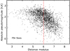 |
Fig. 1. Observed (V,Ks) APMs of 2533 TGAS F5V stars with a parallax error of less than 10%, as a function of their distance modulus. For the stars located at a distance modulus of less than six, the dispersion of the APMs is five times larger than the dispersion due to the photometric and the astrometric noises. Beyond a distance modulus of six, indicated by the vertical red broken line, the APMs begin to decrease. This behavior together with the large APM dispersion may be explained by both multiplicity and observational bias (see text). |
2.1. APM-distance relationship in practice
To derive  from the distribution of APMs, one needs to assert the statistics of the distribution of APMs as a function of distance.
One would naively expect a Gaussian distribution around a value independent of distance. However, as in the example of Fig. 1, this is not the case. Figure 1 shows the observed (V,Ks) APMs of 2533 F5V stars from the TGAS catalog. We selected the stars with a parallax error of less than 10% in order to avoid numerical biases in the conversion process of parallax in distance modulus. Clearly, the APMs have a very large dispersion. For the stars located at a distance modulus smaller than six, the measured dispersion is of the order of 0.5 mag, that is, five times larger than the dispersion induced by the statistical noise, photometric and astrometric, which is of the order of 0.1 mag. This phenomenon can easily be explained by the presence of a large number of multiple stars, mainly twins and triplets, whose effect is to decrease the APMs and therefore to broaden their distribution (see Sect. 2.2). In addition, beyond a distance modulus of six, all the APMs appear to decrease. This decrease is observed for nearly all spectral types and the distance at which it occurs increases with the effective temperature. This effect is mainly due to an observational bias related to the sensitivity limit of the system which detects less and less single stars to the benefit of multiple stars as the distance increases, coupled with an increasing inaccuracy of spectral type identification.
2.2.  estimate procedure
To estimate the  of MS stars, we proceed as follows.
Select all the TGAS MS stars with a parallax error of less than 10%, with or without luminosity class selection depending on the degree of confusion;
for each spectral type, keep only the stars located at a distance smaller than that at which the APMs start to decrease;
fit the resulting APM distributions with a set of three (eventually two or one) Gaussian functions of the same variance;
of the three Gaussian positions, keep that of the single stars, i.e., the highest value, as the
 ’s value.
The model of APM distribution considered at step (3) does not represent the real distribution, as we expect that of multiple stars not to be Gaussian, and with a variance larger than that of single stars. However, it has the great advantage of producing very stable Gaussian positions against the maximum distance of the samples. In this framework, only the ratio between the number of single and multiple stars will vary with the maximum distance. Also, we have made no distinction of age and metallicity as their influence on the APMs is small, in any case smaller than the statistical and systematic errors managed in this work.
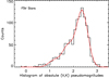 |
Fig. 2. (V,Ks) APM distribution of the 1141 TGAS F5V stars located at a distance modulus smaller than six. The red curve represents the fit of the distribution with three Gaussian functions of the same variance. In this case, the positions of the secondary and the tertiary Gaussian functions are smaller by 0.63 and 1.26 mag with respect to that of the primary Gaussian function. |
We computed the (V,J), (V,H) and (V,Ks)  of MS stars for spectral types B1 to K7, based on the analysis of about 10 000 stars. The median statistical error is of the order of 0.02 mag, but we estimate the systematic error to be 0.05 mag for F, G, and K stars, and 0.1 mag for B and A stars. As an example, Fig. 2 shows the (V,Ks) APM distribution of the selected F5V stars, located at a distance modulus less than six, together with the triple Gaussian fit. Figure 3 represents the (V,Ks) APM distribution for all selected MS stars from B1 to K7 spectral types, the APM distribution of each spectral type having been previously shifted to that of F5V stars. The shape of of the distribution, with a main peak and an extended component on the left, is typical for nearly all spectral types. This is the kind of morphology we expect for the pseudo-photometric distance distribution of a complete open cluster, assuming that the multiplicity frequency is the same as the solar neighborhood.
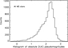 |
Fig. 3. (V,Ks) APM distribution for all spectral types from B1 to K7, the APM distribution of each spectral type having been previously shifted to that of F5V stars. The morphology of this distribution, with a main peak and an extended component to the left, is what we expect for the pseudo-photometric distance distribution of a complete open cluster. |
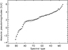 |
Fig. 4. Full circles: (V,Ks) |


Thirty three spectral-type distributions have been fitted with three Gaussian functions. On average, the secondary and the tertiary Gaussians are shifted down by 0.63 ± 0.09 and 1.35 ± 0.24 mag, respectively, with respect to the main Gaussian. These values compare fairly well with 0.75 and 1.19 mag, the maximum downward shifts expected from exact twins and star triplets with respect to single stars. This tends to confirm that the extended component on the left of the main peak is mainly due to multiplicity.
Figure 4 shows the computed (V,Ks)  from O9 to M4 (filled circles). (The values for O9, B0, and K8 to M4 spectral types are taken from our HIPPARCOS data analysis Chelli & Duvert 2016). The broken line represents the HIPPARCOS calibration. The larger differences between the two calibrations, from −0.2 to 0.3 mag, mainly occur for B and A stars.
3. Cluster data retrieval procedures
Our statistical estimate of open cluster distances using pseudomagnitudes is based on the retrieval, cluster per cluster, of a few measurements that must be present for each star: the VJHKs photometries and a spectral type of a relatively high level of precision (one subclass or better). To do this, we first select a list of stars pertaining to each cluster, and then query SIMBAD for each of these stars. As SIMBAD does not provide a compendium of all measurements on stars but only a bibliography-based list of properties, only a subset of all measurements made on open clusters can be retrieved using this procedure. The information returned by SIMBAD is therefore potentially poorer than what one could retrieve from a dedicated database such as WEBDA. We use SIMBAD because it nevertheless provides homogeneous and uniform answers, not to mention its facility of query.
We started with the list of open clusters of Dias et al. (2002) which lists the approximate center coordinates αcl and δcl and angular radius R of 2167 open clusters. Of these, 239 have more than five stars were identified by SIMBAD as pertaining to a stellar cluster: one of the Object Types (OTypes) associated to the star is “*inCl”. Our selection procedure is therefore as follows:
Find in a cone search of radius R around αcl and δcl all the stars known by SIMBAD;
for each star, retrieve V, J, H, Ks spectral type, position, proper motions (the latter preferably using a cross-match with Gaia’s first release Gaia Collaboration 2016a), and the list of associated OTypes;
retain only stars tagged “In Cluster”;
sort the clusters by the number of stars thus returned;
check, by comparing a “finding chart” of the result with one of the cluster’s maps available in WEBDA1, that the circular field of view is not polluted by another cluster’s stars2.
At that point, we obtain only the stars identified as “in Cluster” by SIMBAD. This is not, however, a sure sign of cluster membership. It only means that this star is cited in a publication related to a star cluster. The probability of membership, usually present along with the star’s identification in these publications, is not kept in the process. It is therefore normal that some of the stars retrieved by our procedure do not belong to a cluster. It is easy, nonetheless, based on our pseudo-photometric distances, to find these outliers.
To facilitate the comparison with the distance measurements of fvl17, we merged our lists with the object lists of their 19 clusters. Also, in view of the somewhat poor returns from SIMBAD on some well-known clusters, we searched the Vizier3 catalogs for surveys of particular clusters containing both V photometries and spectral classifications, and merged their object list with the one returned by SIMBAD. This permitted us to add objects to the Praesepe (Patience et al. 2002; Adams et al. 2002), NGC2264 (Venuti et al. 2014), NGC6811 (Peña et al. 2011), Trumpler 16(Wolk et al.2011),NGC2232(Currie et al.2008)and M29 (Milašius et al. 2013) lists. In the case ofM29, the 1774 stars of Milašius et al. (2013) are not specifically identified as belonging to the cluster; in the following, we show that indeed most are field stars at various distances, but we kept this cluster to illustrate that one can make a distance measurement as soon as the histogram of distances exhibits a well-defined peak; see Fig. 8.
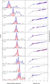 |
Fig. 5. Top: pseudo-photometric distances of 29 open clusters as a function TGAS distances. The black circles represent the clusters of the fvl17 list, except NGC 6633 (18 clusters); the red circles concern 11 additional clusters. The green straight line is the statistical linear fit with the equation ppdm = (0.023 ± 0.047) + (0.999 ± 0.007) × tgdm. Bottom: difference between pseudo-photometric and TGAS distances. |
Comparison between the pseudo-photometric and TGAS distances for the 19 fvl17 clusters.
Comparison between the pseudo-photometric and TGAS distances for 11 additional clusters.
4. Distances of 30 open clusters
In order to derive the distances of our open clusters, we assume that all selected stars are on the MS and we adopt the basic hypothesis of photometric methods. Thereby, we also assume that all the stars share the same photometric properties as their solar neighborhood counterparts in the V, J, H and Ks bands. Large deviations may occur, but only for M stars and those cooler than this. As a consequence, we suppress all M stars from our database.
4.1. Methodology
For each star with known spectral type and VJHKs magnitudes, we compute the three pseudo-photometric distances (V,J), (V,H), and (V,Ks), and their dispersion. We exclude all stars with a distance dispersion larger than 0.1 mag, which allows us to partially filter the sample from non-twin multiples, and we perform a simple average of the three distances. For each cluster, we compute the distances distribution that we fit with one or more Gaussian functions, and then we select the main peak of the distribution. The distance of the cluster is set equal to the mean distance of the stars located within two to three standard deviations (hereafter sd) from the Gaussian position of the selected peak, depending on whether the peak is well isolated or not, and its error is set to the dispersion of the distances divided by the square root of the number of stars.
We compute two distance distributions; the first one (hereafter dd1, 30 clusters) is only based on the pseudo-photometric distances as described above, and the second one (hereafter dd2, 25 clusters) is based on the restricted sample of stars whose proper motion is, within the noise, in agreement with the cluster mean proper motion. For this purpose, we first compute the proper motion distributions in right ascension and declination and we fit these distributions with one or more Gaussian functions. Then, we select the stars located within 3 sd of the main Gaussian peak of the distributions in right ascension and declination, and we continue with the procedure described above. Therefore, for each cluster, we compute two mean pseudo-photometric distances: ppdm1 without, and ppdm2 with, proper motion constraint. The mean positions and the mean proper motions of the clusters are computed from a simple average of the selected ppdm2 stars, or, if the proper motion information is not robust enough to estimate ppdm2 (5 clusters), they are computed from the stars selected to estimate the TGAS distance (see Sect. 5).
For ppdm2 estimates, we first try to use the proper motion measurements from TGAS. When the dd2s contain multiple peaks with no clear choice for the right one and/or when there are too few data for a robust distance estimate, we use HIPPARCOS proper motion. This is the case for Praesepe, NGC 6475, IC 4665, Collinder 140, NGC 2422, NGC 1647, NGC 2264, and M 67. In five cases, NGC 6811, M 29, NGC 869, NGC 884 and Trumpler 16, the proper motion information was not robust enough to estimate ppdm2.
4.2. Distances distribution morphologies
Tables 1 and 2 show the computed pseudo-photometric distances of thirty open clusters, selected from the analysis of more than 200 clusters, and their TGAS distances. The left columns of Figs. 6–8 show the dd1 for the 30 clusters (black histogram) and dd2 (red histogram) for 25 clusters, together with their multiple Gaussian fit; the right columns show the corresponding (V,Ks) pseudomagnitudes as a function of the spectral type and the (V,Ks)  calibration curve shifted at the computed distance (full curve). Most of the distance distributions exhibit a complex structure with extended components and/or multiple peaks. The distance distributions dd1 and/or dd2 of 29 clusters show a clear main peak that we selected to estimate the mean distance moduli. For NGC 2264 data, we find two clusters at different distances (see below).
The dd2s with proper motion constraints (and also dd1) of the Pleiades and Praesepe (Fig. 6), and M 67 (Fig. 8, middle) have a morphology similar to that of the recentered (V,Ks) APM distribution from all TGAS spectral types (see Sect. 2.2 and Fig. 3), that is, a main peak and an extended structure on the left. In addition, if we fit a Gaussian function to the TGAS parallaxes distribution of the stars within and outside 2.5 sd from the main narrow peak, we find comparable mean parallaxes of (7.49 ± 0.04 and 7.50 ± 0.04) and (5.57 ± 0.06 and 5.41 ± 0.05) mas, for the Pleiades and Praesepe, respectively. On the other hand, the dd2s of the two clusters NGC 3532 and NGC 1647 exhibit a triple-peaked structure with secondary and tertiary peaks shifted down by 0.64 and 0.59 mag, 1.27 and 1.11 mag from the main peak, respectively. These shifts are comparable to those expected for twin stars and triplets, that is, 0.75 and 1.19 mag (see Sect. 2.1). In the case of NGC 3532, if we fit with a Gaussian function the TGAS parallax distributions of the stars located within 1.5 sd of each of the three peaks, we find similar parallaxes with Gaussian positions of 2.23 ± 0.02, 2.30 ± 0.03, and 2.19 ± 0.02 mas, for the primary, secondary, and tertiary peaks, respectively. All these results confirm that the extended components and the secondary peaks present in dd2 (and often in dd1 also) are the signature of multiple stars.
The dd2s (eventually dd1s) of some clusters (i.e., the Hyades, IC 2391, IC 2602, NGC 2451, Blanco 1, NGC 2232, and NGC 2547) only show a single, more or less clean peak with a Gaussian sd varying from 0.18 to 0.46 mag. The morphology of the distance distributions of the other clusters is more complex and often intermediate between a single main peak with an extended component at the left and a multiple peaked structure. This is the case for Coma Ber, NGC 6475, NGC 7092, NGC 6633, IC 4665, NGC 2516, Collinder 140, NGC 2422, Stock 2, Collinder 70, NGC 7243, NGC 6811, NGC 869, NGC 884 and Trumpler 16. These morphology differences are probably not due to physical differences between the clusters, but simply to incomplete samples. For M 29, although the list of stars used comes from a survey of a large region around the cluster, the small percentage of genuine M 29 stars is visible as a narrow peak at the cluster’s distance; see also the dd1s of Coma Ber and Collinder 70. At last, we note that the cluster NGC 7092 represents the limit of the exercise, with a small number of sources and multiple peaks. Our derived distance for this cluster, 7.42 ± 0.02, should be considered with caution.
The cluster NGC 2264 has particularly retained our attention because there is some controversy about its distance; see the discussion of Dzib et al. (2014). The dd1, but also dd2, of this cluster exhibit two clear peaks at the two distances 7.49 ± 0.09 and 9.17 ± 0.07 (Fig. 8). As these peaks are too far apart to be due to multiplicity, they must represent two distinct clusters which share the same average position and proper motion (see Table 2).
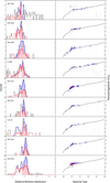 |
Fig. 6. Left: pseudo-photometric distance distributions of open clusters from the list of fvl17 (first part: 10 clusters); black and red histograms: dd1 and dd2, without and with proper motion constraints, respectively (see text); full blue and red lines: Gaussian fits; the blue and red hatched regions correspond to the selected stars used to compute ppdm1 and ppdm2, respectively. Right: black points: (V,Ks) pseudomagnitudes as a function of spectral type; blue and red points: stars used to compute ppdm1 and ppdm2, respectively. |
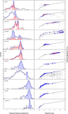 |
Fig. 7. Left: pseudo-photometric distance distributions of open clusters from the list of fvl17 (second part: 9 clusters). Right: (V,Ks) pseudomagnitudes as a function of spectral type. See caption of Fig. 6 for details. |
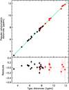 |
Fig. 8. Pseudo-photometric distance distributions of 11 additional open clusters. Left: pseudo-photometric distance distributions. Right: (V,Ks) pseudomagnitudes as a function of spectral type. See caption of Fig. 6 for details. |
4.3. Comparison between distances ppdm1 and ppdm2
The dispersion of the difference between ppdm1 and ppdm2 for the 25 clusters with measured ppdm2 is about 0.04 mag. This small root mean square (rms) difference shows that the selection of the stars labeled “In Cluster” by Simbad, without checking for proper motion, together with the methodology adopted in this paper, allows us, in general, to infer relatively accurate cluster distances. The largest differences are for NGC 3532 (0.13 mag) and, quite strikingly, the Hyades (0.12 mag), which is the closest cluster. For the Hyades, the difference may be explained by its complexity, its very large physical size, and the presence in the sample of stars that even though tagged “In Cluster” do not belong to the cluster. In the following, we retain the pseudo-photometric distances ppdm2 (25 clusters) and, in their absence, ppdm1 (5 clusters); indicated in bold characters in Tables 1 and 2.
4.4 Influence of PMS stars on distance estimates
We have recomputed the pseudo-photometric distances ppdm2s (ppdm1 for the last five clusters) excluding stars whose time of arrival on the main sequence (TAMS) is larger than the age of the cluster. Taking the age of the clusters from the WEBDA database and estimating a typical TAMS in each spectral type bin from the values published in Jung & Kim (2007), we found a ppdm difference smaller than 0.01 mag for 20 clusters containing mainly early type stars. For the other 10 clusters, the distance differences vary between −0.08 (Collinder 70) and 0.04 (Alpha Persei) mag, with a rms value of 0.02 mag. We conclude from the selected samples that stars whose TAMS is larger than the age of the cluster have no or little influence on our distance estimates, the largest deviations being of the order of the systematic errors (see below).
The systematic errors on the cluster distances are mainly due to multiplicity, systematic errors associated with absolute pseudomagnitudes calibration, mismatches between our simple Gaussian model and the real pseudo-photometric distance distributions, spectral type mismatches, and the presence in our samples of stars whose TAMS is larger than the age of the cluster. However, the last point merits a more detailed study with larger samples. We estimate that this systematic error is in general of the order of 0.05 mag.
5. Comparison with TGAS distances
The mean parallaxes of the 19 clusters of Table 1 have been computed from TGAS data by fvl17. The last column of the table represents the equivalent TGAS distance moduli (tgdm) and the associated statistical errors. If we except the cluster NGC 6633, the minimum and maximum differences between the tgdm and our ppdm2 estimates are −0.24 and 0.20 mag, for NGC 2516 and NGC 2451, respectively, and the rms difference (18 clusters) is about 0.10 magnitudes. For NGC 6633, our measured position and proper motion correspond to those of fvl17, but the tgdm and ppdm2 values disagree: 8.13 ± 0.03 and 7.44 ± 0.03, respectively. In addition, there is no peak in the dd2 and dd1 distributions at the position computed by fvl17 (Fig. 7). If we assume that the TGAS distance estimate is correct, this discrepancy may be explained by our poor data sample of NGC 6633 and multiplicity.
We also computed the distance moduli of 11 additional clusters listed in Table 2. For these clusters we were able to estimate a mean TGAS distance as follows: we filtered each sample for proper motion using the procedure described in Sect. 4.1, and we fitted the TGAS parallaxes distribution of the selected stars with one or two Gaussian functions. The parallax of the cluster was set equal to the statistical average of the parallax of the stars located within two or three sd from the position of the main Gaussian, and its error was set to the statistical error. We did not try to apply the sophisticated processing used by fvl17. To evaluate the robustness of our simple approach, we computed the statistical average of the TGAS parallaxes of the 19 clusters of Table 1 from fvl samples, and we compared the corresponding distance moduli to the tgdm values, ending with a rms difference of the order of 0.07 mag. To take into account this difference, we quadratically added a systematic error of 0.07 mag to the statistical error of the 11 clusters considered.
Excluding the cluster NGC 6633, Fig. 5 shows the pseudo-photometric distance modulus estimates ppdm of 29 clusters (24 ppdm2 and 5 ppdm1) as a function of the tgdm derived from TGAS parallaxes (18 tgdm from fvl17 and 11 tgdm from this paper). The equation of the fitted straight line is:
 (5)
(5)
The chi-squared of the fit is 2.5, but if we quadratically add a systematic error of 0.05 mag, it decreases to 1.2. Finally, we found a rms difference of 0.10 mag for the 29 clusters, between the two sets of data. Our distance estimates are in excellent agreement with those derived from TGAS astrometry, which confirms the robustness of the pseudo-photometric distances.
6. Conclusion
Pseudomagnitudes are distance indicators free of interstellar reddening effects. From a statistical analysis of TGAS parallax measurements of about 10 000 stars, we have computed the mean absolute pseudomagnitudes (V,J), (V,H), and (V,K) of MS stars as a function of the spectral type. We used SIMBAD to extract photometric and spectral classification information for stars cataloged as pertaining to ≈200 open clusters. We were able to secure sufficient data to compute the pseudo-photometric distance of 30 open clusters. Except for one cluster, our distances are in good agreement with the TGAS distances within a rms of 0.10 mag. Our approach to estimate distances does not require sophisticated modeling. It is a based on a statistical analysis of quasi purely observational quantities. It can be routinely used in all large-scale surveys where statistical distances on a set of stars, such as an open cluster, are required. This approach may also be advantageously used to study the frequency of multiplicity among stars. The coming release of Gaia DR2 will allow to refine the absolute pseudomagnitude estimates of MS stars and to extend the pseudomagnitude concept to other luminosity classes and larger distances.
Acknowledgments
We wish to thank our anonymous referee for insightful comments. This research has made use of 1) the WEBDA database, operated at the Department of Theoretical Physics and Astrophysics of the Masaryk University, 2) data from the European Space Agency (ESA) mission Gaia (https://www.cosmos.esa.int/gaia), processed by the Gaia Data Processing and Analysis Consortium (DPAC, https://www.cosmos.esa.int/web/gaia/dpac/consortium), 3) NASA’s Astrophysics Data System, 4) the SIMBAD database (Wenger et al. 2000), 5) VizieR catalog access tool (Ochsenbein et al. 2000), CDS, Strasbourg, France and 6) data products from the Two Micron All Sky Survey, which is a joint project of the University of Massachusetts and the Infrared Processing and Analysis Center/California Institute of Technology, funded by the National Aeronautics and Space Administration and the National Science Foundation. We used the TOPCAT4 (Taylor 2005) and STILTS5 (Taylor 2006) tools to easily manipulate the star databases used.
In the rare cases it happened, a spatial handmade selection with TopCat removed the spurious stars.
Available at http://www.starlink.ac.uk/topcat
Available at http://www.starlink.ac.uk/stilts
References
- Abbott, B. P., Abbott, R., Abbott, T. D., et al. 2017, ApJ, 851, L35 [NASA ADS] [CrossRef] [Google Scholar]
- Adams, J. D., Stauffer, J. R., Skrutskie, M. F., et al. 2002, AJ, 124, 1570 [NASA ADS] [CrossRef] [Google Scholar]
- Bourges, L., Mella, G., Lafrasse, S., et al. 2017, VizieR Online Data Catalog: II/346 [Google Scholar]
- Chelli, A., Bourges, L., Duvert, G., et al. 2014, in Proc. SPIE, 9146, 91462Z [CrossRef] [Google Scholar]
- Chelli, A., & Duvert, G. 2016, A&A, 593, L18 [NASA ADS] [CrossRef] [EDP Sciences] [Google Scholar]
- Chelli, A., Duvert, G., Bourgès, L., et al. 2016, A&A, 589, A112 [NASA ADS] [CrossRef] [EDP Sciences] [Google Scholar]
- Currie, T., Plavchan, P., & Kenyon, S. J. 2008, ApJ, 688, 597 [NASA ADS] [CrossRef] [Google Scholar]
- Dias, W. S., Alessi, B. S., Moitinho, A., & Lépine, J. R. D. 2002, A&A, 389, 871 [NASA ADS] [CrossRef] [EDP Sciences] [Google Scholar]
- Dzib, S. A., Loinard, L., Rodríguez, L. F., & Galli, P. 2014, ApJ, 788, 162 [NASA ADS] [CrossRef] [Google Scholar]
- ESA 1997, The Hipparcos and Tycho Catalogues, ESA SP-1200, 1 [Google Scholar]
- Fitzpatrick, E. L. 1999, PASP, 111, 63 [NASA ADS] [CrossRef] [Google Scholar]
- Gaia Collaboration (Brown, A. G. A., et al.) 2016a, A&A, 595, A2 [NASA ADS] [CrossRef] [EDP Sciences] [Google Scholar]
- Gaia Collaboration (Prusti, T., et al.) 2016b, A&A, 595, A1 [NASA ADS] [CrossRef] [EDP Sciences] [Google Scholar]
- Gaia Collaboration (van Leeuwen, F., et al.) 2017, A&A, 601, A19 [NASA ADS] [CrossRef] [EDP Sciences] [Google Scholar]
- Jung, Y. K., & Kim, Y.-C. 2007, J. Astron. Space Sci., 24, 1 [NASA ADS] [CrossRef] [Google Scholar]
- Lang, R. N., & Hughes, S. A. 2008, ApJ, 677, 1184 [NASA ADS] [CrossRef] [Google Scholar]
- Madore, B. F. 1982, ApJ, 253, 575 [NASA ADS] [CrossRef] [Google Scholar]
- Melis, C., Reid, M. J., Mioduszewski, A. J., Stauffer, J. R., & Bower, G. C. 2014, Science, 345, 1029 [NASA ADS] [CrossRef] [PubMed] [Google Scholar]
- Milašius, K., Boyle, R. P., Vrba, F. J., et al. 2013, Baltic Astron., 22, 181 [NASA ADS] [Google Scholar]
- Ochsenbein, F., Bauer, P., & Marcout, J. 2000, A&AS, 143, 23 [NASA ADS] [CrossRef] [EDP Sciences] [Google Scholar]
- Patience, J., Ghez, A. M., Reid, I. N., & Matthews, K. 2002, AJ, 123, 1570 [NASA ADS] [CrossRef] [Google Scholar]
- Peña, J. H., Fox Machado, L., García, H., et al. 2011, RM&AC, 47, 309 [Google Scholar]
- Taylor, M. B. 2005, in ASP Conf. Ser., 347, 29 [Google Scholar]
- Taylor, M. B. 2006, in ASP Conf. Ser., 351, 666 [Google Scholar]
- van den Bergh, S. 1975, The Extragalactic Distance Scale, eds. Sandage, A. Sandage, M. & Kristian J. (University of Chicago Press), 509 [Google Scholar]
- van Leeuwen, F. 2007, A&A, 474, 653 [NASA ADS] [CrossRef] [EDP Sciences] [Google Scholar]
- Venuti, L., Bouvier, J., Flaccomio, E., et al. 2014, A&A, 570, A82 [NASA ADS] [CrossRef] [EDP Sciences] [Google Scholar]
- Wenger, M., Ochsenbein, F., Egret, D., et al. 2000, A&AS, 143, 9 [NASA ADS] [CrossRef] [EDP Sciences] [Google Scholar]
- Wolk, S. J., Broos, P. S., Getman, K. V., et al. 2011, ApJS, 194, 12 [NASA ADS] [CrossRef] [Google Scholar]
All Tables
Comparison between the pseudo-photometric and TGAS distances for the 19 fvl17 clusters.
Comparison between the pseudo-photometric and TGAS distances for 11 additional clusters.
All Figures
|
Fig. 1. Observed (V,Ks) APMs of 2533 TGAS F5V stars with a parallax error of less than 10%, as a function of their distance modulus. For the stars located at a distance modulus of less than six, the dispersion of the APMs is five times larger than the dispersion due to the photometric and the astrometric noises. Beyond a distance modulus of six, indicated by the vertical red broken line, the APMs begin to decrease. This behavior together with the large APM dispersion may be explained by both multiplicity and observational bias (see text). |
| In the text | |
|
Fig. 2. (V,Ks) APM distribution of the 1141 TGAS F5V stars located at a distance modulus smaller than six. The red curve represents the fit of the distribution with three Gaussian functions of the same variance. In this case, the positions of the secondary and the tertiary Gaussian functions are smaller by 0.63 and 1.26 mag with respect to that of the primary Gaussian function. |
| In the text | |
|
Fig. 3. (V,Ks) APM distribution for all spectral types from B1 to K7, the APM distribution of each spectral type having been previously shifted to that of F5V stars. The morphology of this distribution, with a main peak and an extended component to the left, is what we expect for the pseudo-photometric distance distribution of a complete open cluster. |
| In the text | |
|
Fig. 4. Full circles: (V,Ks) |
| In the text | |
|
Fig. 5. Top: pseudo-photometric distances of 29 open clusters as a function TGAS distances. The black circles represent the clusters of the fvl17 list, except NGC 6633 (18 clusters); the red circles concern 11 additional clusters. The green straight line is the statistical linear fit with the equation ppdm = (0.023 ± 0.047) + (0.999 ± 0.007) × tgdm. Bottom: difference between pseudo-photometric and TGAS distances. |
| In the text | |
|
Fig. 6. Left: pseudo-photometric distance distributions of open clusters from the list of fvl17 (first part: 10 clusters); black and red histograms: dd1 and dd2, without and with proper motion constraints, respectively (see text); full blue and red lines: Gaussian fits; the blue and red hatched regions correspond to the selected stars used to compute ppdm1 and ppdm2, respectively. Right: black points: (V,Ks) pseudomagnitudes as a function of spectral type; blue and red points: stars used to compute ppdm1 and ppdm2, respectively. |
| In the text | |
|
Fig. 7. Left: pseudo-photometric distance distributions of open clusters from the list of fvl17 (second part: 9 clusters). Right: (V,Ks) pseudomagnitudes as a function of spectral type. See caption of Fig. 6 for details. |
| In the text | |
|
Fig. 8. Pseudo-photometric distance distributions of 11 additional open clusters. Left: pseudo-photometric distance distributions. Right: (V,Ks) pseudomagnitudes as a function of spectral type. See caption of Fig. 6 for details. |
| In the text | |
Current usage metrics show cumulative count of Article Views (full-text article views including HTML views, PDF and ePub downloads, according to the available data) and Abstracts Views on Vision4Press platform.
Data correspond to usage on the plateform after 2015. The current usage metrics is available 48-96 hours after online publication and is updated daily on week days.
Initial download of the metrics may take a while.