© ESO 2018

1. Introduction

For about a decade, the modern time-delay cosmography, namely the cosmological parameter inferences from time delay measurements in strong gravitational lensing, have been achieved with an increasingly competitive precision (for a recent review, Treu & Marshall 2016; see and references therein). A crucial step of this technique relies upon a robust characterization of the gravitational potential, which produces the multiply imaged configuration of a background bright quasar (see, e.g., Keeton 2003; Fassnacht et al. 2006; Suyu et al. 2010, 2013; Wong et al. 2011; Wong et al. 2017; Birrer et al. 2016). This gravitational potential is essentially produced by a main deflector but also by any mass distributions lying along the line of sight to the source (Seljak 1994; Bar-Kana 1996). Unfortunately, modeling the main lens mass distribution faces a major hurdle, namely the existence of degeneracies between plausible lens density profiles. In fact, significant freedom exists in choosing lens models that produce the same image configurations but predict different products of time delays and Hubble constant, H₀ Δt (Schneider & Sluse 2013). Thus, these degeneracies translate into systematic errors that propagate to H₀.

Now well-known to the lensing community, the first lensing invariance to have been pointed out is the mass-sheet degeneracy (MSD; Falco et al. 1985). A dimensionless surface mass density κ(θ) and all the modified κ_λ(θ) under the mass-sheet transformation (MST) defined as

$$\begin{array}{c}\hfill {\kappa }_{\lambda }(\mathit{\theta })=\lambda \kappa (\mathit{\theta })+(1-\lambda ),\end{array}$$(1)

along with the corresponding unobservable source rescaling β → λ β, lead to identical lensing observables with the exception of time delays, which transform as in Δt → λ Δt. This pure mathematical degeneracy has nothing to do with the gravitational perturbations caused by external masses along the line of sight. Whereas various solutions have been already proposed to reduce the impact of the MST on time-delay cosmography (see, e.g., Sect. 3 in Treu & Marshall 2016; and references therein), none of them succeed in unambiguously breaking the MSD. The source position transformation (SPT), a more general class of degeneracies which includes the MST as a special case, has been introduced in Schneider & Sluse (2014) and carried forward in Unruh et al. (2017). The SPT defines a new mathematical framework that includes degeneracies that have been neither described nor considered in time-delay cosmography before. The first estimation of its impact on time delays is given in Schneider & Sluse (2014) where the authors show experimentally that predictions for H₀ can deviate by ∼20% when comparing a softened power law (SPL) with a composite (baryons + dark matter) lens models. However, this value has been overestimated owing to a bug in the software used by the author. We address this issue in Sect. 5 and show that the predictions for H₀ can deviate by ∼7% instead.

Recently, a detailed analysis of how the SPT may affect the time-delay cosmography has been presented in Wertz et al. (2018). To address this question, we started by developing a flexible numerical framework that encompasses well-tested and efficient implementations of most of the analytical results published in Schneider & Sluse (2014) and Unruh et al. (2017). Numerous additional features were then added, giving rise to pySPT, an easy-to-use and well-documented python package dedicated to the SPT. We used pySPT to draw the conclusions presented in Wertz et al. (2018). Thus, our package is released as open source, making our results easy to reproduce. Beyond that, we also hope that it will be useful to the time-delay cosmography community to quantify the systematic errors that are introduced by the SPT when inferring H₀.

This paper is organized as follows. We outline the basic principles of SPT in Sect. 2. Section 3 gives an overall description of the package design and features, and details are provided in Sect. 4. In Sect. 5, we present the corrected version of some results presented in Schneider & Sluse (2014). We summarize our findings in Sect. 6.

2. Principle of source position transformation

This section focuses on the basic idea underlying the SPT and its mathematical framework. A detailed discussion is provided in Schneider & Sluse (2014) and Unruh et al. (2017). In this paper we adopt the standard gravitational lensing notation (see Schneider 2006).

The relative lensed image positions θ_i(θ₁) of a background point-like source located at the unobservable position β constitute the lensing observables that we measure with the highest accuracy and precision. As a typical example, just a few mas can be achieved with deep HST observations. When n images are observed, the mapping θ_i(θ₁) only provides the constraints

$$\begin{array}{c}\hfill {\mathit{\theta }}_i-\mathit{\alpha }({\mathit{\theta }}_i)={\mathit{\theta }}_j-\mathit{\alpha }({\mathit{\theta }}_j),\forall 1\le i<j\le n,\end{array}$$(2)

where α(θ) corresponds to the deflection law caused by a foreground surface mass density κ(θ), the so-called lens. The SPT addresses the question of whether we define an alternative deflection law, denoted as $\widehat{\mathit{\alpha }}(\mathit{\theta })$, which preserves the mapping θ_i(θ₁) for a unique source? If such a deflection law exists, the alternative source position $\widehat{\mathit{\beta }}$ differs in general from β. Furthermore, it defines the new lens mapping $\widehat{\mathit{\beta }}=\mathit{\theta }-\widehat{\mathit{\alpha }}(\mathit{\theta })$, which leads to

$$\begin{array}{c}\hfill \mathit{\theta }=\mathit{\beta }+\mathit{\alpha }(\mathit{\theta })=\widehat{\mathit{\beta }}+\widehat{\mathit{\alpha }}(\mathit{\theta }).\end{array}$$(3)

An SPT consists in a global transformation of the source plane formally defined by a one-to-one mapping $\widehat{\mathit{\beta }}(\mathit{\beta })$, unrelated to any physical contribution such as the external convergence (Schneider & Sluse 2013). To preserve the mapping θ_i(θ₁), the alternative deflection law is thus written

$$\begin{array}{c}\hfill \widehat{\mathit{\alpha }}(\mathit{\theta })=\mathit{\alpha }(\mathit{\theta })+\mathit{\beta }-\widehat{\mathit{\beta }}(\mathit{\beta })=\mathit{\alpha }(\mathit{\theta })+\mathit{\beta }-\widehat{\mathit{\beta }}(\mathit{\theta }-\mathit{\alpha }(\mathit{\theta })),\end{array}$$(4)

where in the first step we used Eq. (3) and in the last step we inserted the original lens equation. As defined, the deflection laws α(θ) and $\widehat{\mathit{\alpha }}(\mathit{\theta })$ yield exactly the same image positions of the source β and $\widehat{\mathit{\beta }}$, respectively.

Because $\widehat{\mathit{\alpha }}$ is in general not a curl-free field, it cannot be expressed as the gradient of a deflection potential caused by a mass distribution κ̂. Provided its curl component is sufficiently small, Unruh et al. (2017) have established that one can find a curl-free deflection law ᾶ = ∇ψ̃ that is similar to $\widehat{\mathit{\alpha }}$ in a finite region. In other words, ᾶ yields the same sets of multiple images up to the astrometric accuracy ε_acc of current observations. Two image configurations are considered indistinguishable when they satisfy

$$|\Delta \theta |\hspace{0.17em}:=\left|\tilde{\theta }-\theta \right|<{\epsilon }_{\text{acc}},$$(5)

for all images θ of the source β, and corresponding images θ̃ of the source $\widehat{\mathit{\beta }}$ with $\tilde{\mathit{\theta }}=\widehat{\mathit{\beta }}+\tilde{\mathit{\alpha }}(\tilde{\mathit{\theta }})$. In Unruh et al. (2017), the adopted similarity criterion is written

$$|\Delta \alpha (\theta )|\hspace{0.17em}:=\hspace{0.17em}|\tilde{\alpha }(\theta )-\widehat{\alpha }(\theta )|\hspace{0.17em}<{\epsilon }_{\text{acc}},$$(6)

in a finite region of the lens plane denoted as 𝒰 where multiple images occur. Even though this criterion cannot actually guarantee |Δθ|< ε_acc over 𝒰, there exists in general a subregion 𝒰′⊂𝒰 that includes image configurations for which Eq. (5) is satisfied (see Sect. 4.1 in Wertz et al. 2018). Thus, an SPT $\widehat{\mathit{\beta }}(\mathit{\beta })$ leads to an alternative lens profile κ̂, which gives rise to the SPT-transformed deflection law $\widehat{\mathit{\alpha }}$, then its curl-free counterpart ᾶ is defined based upon the criterion Eq. (6), and may lead to indistinguishable image configurations produced by α. To conclude this section, we note that the deflection law ᾶ is produced by a surface mass density κ̃ := ∇ · ᾶ/2, which equals κ̂ by construction.

3. Package overview

The pySPT program was developed in python (Watters et al. 1996) and only relies on packages included in the python standard library¹ and the proven open-source libraries numpy (Van Der Walt et al. 2011), scipy (Jones et al. 2001), and matplotlib (Hunter 2007). The code design and development follow effective practices for scientific computing such as using test cases and a profiler to identify bugs and bottlenecks, keeping an effective collaboration thanks to a version control system (git), and providing an extensive documentation (Wilson et al. 2014). This open source code is available on GitHub² and comes along with a clear description on how to install it. To make the best use out of pySPT, a quick start guide and several tutorials are also provided in the form of Jupyter notebooks. Benefiting from the python object-oriented paradigm, the structure of pySPT is highly modular, which avoids code clones and makes it less sensitive to bug propagation.

The code is composed of several modules built from various classes and is organized in a dozen subpackages. Its core is separated into three main subpackages, referred to as lensing, sourcemapping, and spt The reason for that is simple. The mapping $\widehat{\mathit{\beta }}(\mathit{\beta })$ presented in Sect. 2 defines a one-to-one connection between the source plane and its SPT-transformed counterpart. Through the lens equation β = θ − α(θ), the deflection law (arising from a lens model) characterizes the link between the source plane and the image plane. Thus, only together with α(θ) does $\widehat{\mathit{\beta }}(\mathit{\beta })$ give rise to the alternative deflection law $\widehat{\mathit{\alpha }}(\mathit{\theta })$ defined in Eq. (4). As a result, the most significant pySPT subpackages are lensing to basically deal with α(θ), sourcemapping to define $\widehat{\mathit{\beta }}(\mathit{\beta })$, and spt to describe $\widehat{\mathit{\alpha }}(\mathit{\theta })$ (and all the SPT-transformed lensing quantities). In the remainder of this section, we describe briefly their main functionalities³.

The subpackage lensing shares a lot of functionalities with other lensing-dedicated softwares such as gravlens (Keeton 2001b). From its class Model, we generated a lens model object that allowed us to perform a wide range of basic lensing calculations. Strictly speaking, this part of the code is not related to the SPT and it can be used independent of any SPT analysis. Nevertheless, we decided to implement this part of the code for a simple reason: as a built-in feature of pySPT, the class Model provides to its instances the adequate structure that is required to match the spt requirements. This makes lensing more convenient to use than a third party code. The subpackage sourcemapping is used to define an SPT $\widehat{\mathit{\beta }}(\mathit{\beta })$. Several forms of $\widehat{\mathit{\beta }}(\mathit{\beta })$ are implemented, such as particular radial stretchings presented in Schneider & Sluse (2014). Moreover, the code is designed to accept any user-defined SPT. With sourcemapping also comes functionalities to characterize the mapping $\widehat{\mathit{\beta }}(\mathit{\beta })$, such as testing whether it is one-to-one over a given region. More details are given in Sect. 4.2. The subpackage spt is the heart of pySPT. It is designed to work alongside with sourcemapping and lensing to provide all the basic SPT-transformed quantities, such as $\widehat{\kappa },\hspace{0.17em}\widehat{\alpha },\hspace{0.17em}\widehat{\psi },\hspace{0.17em}\widehat{\mathcal{A}},\hspace{0.17em}\tilde{\theta },\hspace{0.17em}\tilde{\alpha },\hspace{0.17em}\tilde{\psi }$. One can also derive the SPT-transformed time delays Δt̂ and Δt̃, and most of the quantities presented in Schneider & Sluse (2014), Unruh et al. (2017), and Wertz et al. (2018). This makes the results presented in these papers straightforward to reproduce. A detailed description of the tools provided by spt is given in Sect. 4.3.

The pySPT code also includes several subpackages dedicated to specific tasks. Based on the package multiprocessing of the standard library, multiproc provides an efficient tool to parallelize functions and methods in a straightforward way. As such, most of the pySPT features support parallel computing to leverage multiple processors fully. The grid feature helps us to create different types of mesh grids. These are of practical interest for generating maps of lensing quantities in a particular region. To calculate ᾶ efficiently, we followed Unruh et al. (2017), which suggests using a Riemann mapping to handle a pole numerically. Thus, pySPT contains the subpackage integrals that includes functionalities to deal with and to illustrate conformal mappings.

4. Analyzing the impact of the SPT with pySPT

4.1. Subpackage lensing to deal with lens models

To analyze how the SPT may alter lensing observables in a quantitative way, we needed to select a model that characterizes a mass distribution. A range of lensing observables were then generated and compared against those produced by an SPT-transformed version of the original model. The subpackage lensing relies on the class Model of which one of its instances defines a lens model and provides efficient tools to compute a wide range of lensing quantities. Most of the mass profiles described in Keeton (2001a) are available in the subpackage catalog, together with a complete documentation. We note that, to our knowledge, no analytical expression of the deflection potential for the generalized pseudo-NFW can be found in the literature. Hence, we derived this expression and provide the result in Appendix A. The class Model is also designed to accept a user-defined lens model, as long as some conventions are respected. At least, the deflection potential ψ(θ) must be provided as either a python function or a C shared library. Those that are not defined among α, κ, and ∂α/∂θ are then computed from numerical approximation at the expense of a more intensive usage of computer resources. Thanks to operator overloading⁴, arbitrarily complicated composite models can be obtained by simply adding several Model instances. For example, this feature is used to generate quadrupole models, namely the combination of an axisymmetric matter distribution plus some external shear. To go a step further, the axisymmetric part may itself be composed of different components, whereas additional contributions can be included at arbitrary positions.

The computational methods implemented with the class Model follow the prescription of Keeton (2001b). In particular, the so-called tiling algorithm (with adaptive grid) is used to solve the lens equation and locate the critical curves. Other fundamental lensing quantities are available, such as the caustics, basic image properties (e.g., image type, magnification factor, parity, odd-number, and magnification theorem checks), Fermat potential τ(θ), and time delays between image pairs Δt(θ_i, θ_j)≡Δt_ij. In Fig. 1, we illustrate the capabilities of the subpackage lensing by showing several lensing quantities produced by a complex mass distribution. The workflow for generating data used in this figure is as follows⁵:

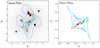Fig. 1. Example illustrating some capabilities of the subpackage lensing. Left panel: eight lens profiles with different parameters are combined to generate a complex mass distribution. The total surface mass density is shown in tones of gray and dashed curves highlight few particular iso-density contours. The colored thick curves show the critical curves and the filled and empty markers locate the lensed image positions of two different sources shown in the right panel. The inverted triangles correspond to images of type I (maximum of τ), the diamonds to type II (saddle point of τ), and triangles to type III (maximum of τ). The size of the markers is log-proportional to the magnification of the images. Right panel: the colored lines show the caustics and the two squares locate the sources. The filled (resp. empty) square has seven (resp. nine) images, all shown in the left panel. The axis scale is arcseconds but unit of θE can also be used.

The subpackage lensing also includes C shared libraries that implement ψ, α, κ, ∂α/∂θ for all the lens models. As shown in Sect. 4.3, the curl-free deflection angle ᾶ is obtained by means of line and surface integrals of functions that involve $\widehat{\mathit{\alpha }}$ (see Eq. (4)) and $\widehat{\kappa }=\mathbf{\nabla }·\widehat{\mathit{\alpha }}/2$ (Unruh et al. 2017). Thus, the original deflection angle α is evaluated as many times as the number of iterations required by the solver to converge. Even though this procedure is efficient when only one ᾶ is evaluated, high performance becomes critical when ᾶ needs to be evaluated on a dense grid. Thanks to the foreign function interface module ctypes⁶, the use of the C shared libraries speeds up significantly the execution of pure python code. The pySPT code comes along with a tutorial in the form of a Jupyter notebook that describes in details how to deal with C shared libraries.

4.2. Defining $\widehat{\mathit{\beta }}(\mathit{\beta })$ with the subpackage sourcemapping

After we defined the lens model, we chose an SPT by defining a source mapping $\widehat{\mathit{\beta }}\equiv \widehat{\mathit{\beta }}(\mathit{\beta })$. To each position β of the source plane, this mapping associates a new and unique position $\widehat{\mathit{\beta }}$ in the source plane. The so-called radial stretching is simply defined as

$$\begin{array}{c}\hfill \widehat{\mathit{\beta }}(\mathit{\beta })=[1+f(|\mathit{\beta }|)]\mathit{\beta },\end{array}$$(7)

where f is called the deformation function. With $\widehat{\mathit{\beta }}$ defined this way, $\widehat{\mathit{\beta }}({\mathit{\beta }}_j)$ always lies on the line passing through 0 and β_j. The most simple case of radial stretching corresponds to a constant deformation function, f(|β|) = λ − 1 with λ ∈ ℝ, which leads to the well-known MST, $\widehat{\mathit{\beta }}=\lambda \mathit{\beta }$. In Wertz et al. (2018), we focused most of the work on the radial stretching Eq. (7) where the deformation function f(|β|) is defined as the lowest order expansion of more general functions

$$\begin{array}{c}\hfill f(|\mathit{\beta }|)=f_0+\frac{f_2}{2{\theta }_{\text{E}}^2}{|\mathit{\beta }|}^2,\end{array}$$(8)

where $f_0:=f(0),f_2:={\theta }_{\text{E}}^2\hspace{0.17em}{f}^{″}(0),{\theta }_{\text{E}}$ is the Einstein angular radius, and f is an even function of |β| to preserve the symmetry (Schneider & Sluse 2014). When f₂ = 0, this case simplifies to a pure MST with λ = 1 + f₀. In Table 1, we provide a list of the radial stretchings implemented in sourcemapping. The rationale behind the choice of these particular deformation functions are motivated in Schneider & Sluse (2014). The first column refers to the id used to identify which source mapping one wants to select. A specific example is given below. Aside from defining an SPT, sourcemapping also includes a few functionalities for characterizing the mapping $\widehat{\mathit{\beta }}(\mathit{\beta })$. In particular, one can test whether the source mapping is one to one over a given region, compute the Jacobi matrix $\mathcal{B}(\mathit{\beta })=\partial \widehat{\mathit{\beta }}(\mathit{\beta })/\partial \mathit{\beta }$, and provide its decomposition ℬ(β)=B₁ℐ + B₂Γ(η), which is useful to evaluate the amplitude of the curl component of $\widehat{\mathit{\alpha }}$ (see Sect. 4.1 in Schneider & Sluse 2014). As an example, the code below illustrates how to define and characterize an MST with λ = 1(≡1 + f₀): Similarly, we can first define the deformation function f that characterizes an MST with λ as unique argument, and pass it to sourcemapping as an argument. For efficiency, the first derivative f′ of the deformation function with respect to |β| can also be passed⁷. This process illustrates how we can work with a user-defined SPT.

4.3. Deriving SPT-transformed quantities with spt

In the two previous sections, we have shown how to generate lensing observables produced by a given lens model and how to define an SPT. We present the subpackage spt, which provides the tools required to determine the SPT-transformed quantities $\widehat{\kappa },\hspace{0.17em}\widehat{\alpha },\hspace{0.17em}\widehat{\psi },\hspace{0.17em}\widehat{\mathcal{A}},\hspace{0.17em}\Delta \widehat{t},\hspace{0.17em}\tilde{\alpha },\hspace{0.17em}\tilde{\psi },\hspace{0.17em}\tilde{\theta },\hspace{0.17em}\text{and}\hspace{0.17em}\Delta \tilde{t}$.

For any SPT and lens model, the alternative deflection law $\widehat{\mathit{\alpha }}$ is implemented as defined in Eq. (4), and the Jacobi matrix of the alternative lens equation given in Eq. (3) as $\widehat{\mathcal{A}}(\mathit{\theta })=(\partial \widehat{\mathit{\beta }}/\partial \mathit{\beta })(\partial \mathit{\alpha }/\partial \mathit{\theta })\equiv \mathcal{B}(\mathit{\beta }(\mathit{\theta }))\mathcal{A}(\mathit{\theta })$. The determination of $\widehat{\mathcal{A}}$ perfectly illustrates how spt works along with lensing and sourcemapping: ℬ(β) is obtained with sourcemapping, β(θ) and 𝒜(θ) are obtained with lensing, and spt combines the results to derive $\widehat{\mathcal{A}}(\mathit{\theta })$. In the axisymmetric case, $\widehat{\mathit{\alpha }}$ is a curl-free field and there exists a deflection potential $\widehat{\psi }$ such that $\text{d}\widehat{\psi }(\theta )/\text{d}\theta =\widehat{\alpha }(\theta )=\theta -\widehat{\beta }(\theta -\alpha (\theta )),$ where θ = |θ|. Thus, $\widehat{\psi }$ is obtained as follows:

$$\begin{array}{c}\hfill \widehat{\psi }(\theta )={\int }_0^{\theta }[\vartheta -\widehat{\beta }(\vartheta -\alpha (\vartheta ))]\text{d}\vartheta ,\end{array}$$(9)

up to a constant independent of θ. Because the integrand in Eq. (9) depends on the SPT and the lens model choices, no general analytical solution can be derived. The integral is therefore computed numerically using the python module integrate.quad⁸ from scipy (Jones et al. 2001). Under a radial stretching, the axisymmetric mass profile κ(θ) transforms into $\widehat{\kappa }(\theta )=\kappa (\theta )-[1-\kappa (\theta )]f(\beta (\theta ))-\theta \text{det}\mathcal{A}(\theta )f\prime (\beta (\theta ))/2$, where β = |β| (Schneider & Sluse 2014). Otherwise, the more general form $\widehat{\kappa }(\mathit{\theta })=1-\text{Tr}(\widehat{\mathcal{A}})/2$ is valid regardless of the lens model symmetry.

When the axisymmetry assumption for the original lens model is dropped, spt also provides the physically meaningful ᾶ and ψ̃. The analytical expressions implemented in SPT are slightly simplified versions of those first presented in Unruh et al. (2017). The deflection potential ψ̃ evaluated at the position θ in the lens plane is explicitly written

$$\begin{array}{c}\hfill \tilde{\psi }(\mathit{\theta })=\langle \tilde{\psi }\rangle +2{\int }_{\mathcal{U}}{H}_1(\mathit{\theta };\mathit{\vartheta })\widehat{\kappa }(\mathit{\vartheta })\hspace{0.17em}{\text{d}}^2\vartheta -{\int }_{\partial \mathcal{U}}{H}_2(\mathit{\theta };\mathit{\vartheta })\widehat{\mathit{\alpha }}·\mathit{n}\hspace{0.17em}\text{d}s,\end{array}$$(10)

where the region 𝒰 is a disk of radius R, 〈ψ̃〉 is the average of ψ̃ on 𝒰, ds the line element of the boundary curve ∂𝒰,

$$\begin{array}{c}\hfill H_1(\mathit{\theta };\mathit{\vartheta })=\frac{1}{4\pi }[ln\left(\frac{{|\mathit{\vartheta }-\mathit{\theta }|}^2}{R^2}\right)+ln(1-\frac{2\mathit{\vartheta }·\mathit{\theta }}{R^2}+\frac{{|\mathit{\vartheta }|}^2{|\mathit{\theta }|}^2}{R^4})-\frac{{|\mathit{\vartheta }|}^2}{R^2}],\end{array}$$(11)

and

$$\begin{array}{c}\hfill H_2(\mathit{\theta };\mathit{\vartheta })=\frac{1}{4\pi }[2ln\left(\frac{{|\mathit{\vartheta }-\mathit{\theta }|}^2}{R^2}\right)-1].\end{array}$$(12)

In Appendix B, we explicitly show that both versions are fully equivalent. The corresponding simplified version of the deflection angle ᾶ can be derived by obtaining the gradient of H₁ and H₂ with respect to θ, which is written

$$\begin{array}{cc}\hfill \tilde{\mathit{\alpha }}(\mathit{\theta })& =\frac{1}{\pi }{\int }_{\mathcal{U}}(\frac{\mathit{\theta }-\mathit{\vartheta }}{{|\mathit{\theta }-\mathit{\vartheta }|}^2}+\frac{{|\mathit{\vartheta }|}^2\mathit{\theta }-R^2\mathit{\vartheta }}{R^4-2R^2\mathit{\vartheta }·\mathit{\theta }+{|\mathit{\vartheta }|}^2{|\mathit{\theta }|}^2})\widehat{\kappa }(\mathit{\vartheta }){\text{d}}^2\vartheta \hfill \\ \hfill & -\frac{1}{\pi }{\int }_{\partial \mathcal{U}}\frac{\mathit{\theta }-\mathit{\vartheta }}{{|\mathit{\theta }-\mathit{\vartheta }|}^2}\widehat{\mathit{\alpha }}·\mathit{n}\text{d}s.\hfill \end{array}$$(13)

To deal with the pole ϑ = θ in the first term of Eqs. (11) and (13), we used a Riemann mapping as described in Appendix A in Unruh et al. (2017) and implemented in the subpackage integrals. This mathematical trick makes the previous integrals easier to solve by mapping 𝒰 onto the unit disk in the complex plane, such as the pole is moved at the origin⁹z = 0. Additional care is however needed in the vicinity of θ = 0, where the gradient of κ(θ) may vary significantly and produce a second sharp peak of the integrand. This peak may even be a new pole when κ is singular at the origin. Thus, a physically meaningful lens model should always be favored. In the left panel in Fig. 2, we illustrate the integrand¹⁰ $|\mathit{\vartheta }|\widehat{\kappa }(\mathit{\vartheta })ln({|\mathit{\vartheta }-\mathit{\theta }|}^2/R^2)$ of the first term of the integral over 𝒰 defined in Eq. (10). For this illustrative example, we choose an non-singular isothermal sphere (NIS, θ_c = 0.1θ_E) lens model plus external shear (γ_p = 0.1) transformed by the radial stretching $\widehat{\mathit{\beta }}(\mathit{\beta })=f_0+f_2{|\mathit{\beta }|}^2/(2{\theta }_{\text{E}}^2)$ with (f₀, f₂)=(0, 0.55) and θ = ( − 0.5, 0.25) θ_E. The negative peak comes from the pole ϑ = θ while the central peak is caused by κ(|ϑ|=0). The right panel in Fig. 2 illustrates the integrand after applying the Riemann mapping. The peaks have moved and the pole ϑ = θ now lies at the origin z = 0, as expected. To deal with the second peak, the subpackage integrals splits the integration domain to place it on a boundary and to ensure the gradient of the integrand is smooth in the sub\domains.

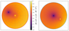Fig. 2. Representative example that illustrates how the integration domain 𝒰 is mapped onto the unit disk in the complex plane under a Riemann mapping. Left panel: the color coding depicts the integrand $|\mathit{\vartheta }|\widehat{\kappa }{(\mathit{\vartheta })ln(|\mathit{\vartheta }-\mathit{\theta }|}^2/R^2)$ for all ϑ ∈ 𝒰. It shows a pole at ϑ = θ with θ = ( − 0.5, 0.25) θE and a secondary peak at the origin caused by κ(|ϑ|=0). The lens model is an NIS (θc = 0.1θE) plus external shear (γp = 0.1) transformed by the radial stretching $\widehat{\mathit{\beta }}(\mathit{\beta })=f_0+f_2{|\mathit{\beta }|}^2/(2{\theta }_{\text{E}}^2)$ with (f0, f2)=(0, 0.55). The red circle delimits 𝒰 with radius R. Right panel: integrand after applying the Riemann mapping described in Appendix A in Unruh et al. (2017). The pole ϑ = θ now lies at the origin of the unit (blue) circle of the complex plane. The polar grid (gray lines) allows us to visualize how the Riemann mapping acts on 𝒰. For this figure, we used the subpackage integrals that addresses both the pole and second peak.

With $\widehat{\mathit{\alpha }}$ and ᾶ, we can evaluate the SPT validity criterion adopted in Unruh et al. (2017) and recalled in Eq. (6). With the same lens model and SPT adopted for Figs. 2 and 3 shows the map |Δα(θ)| over a circular grid |θ| ≤2 θ_E in the lens plane. It is worth noting that this figure is similar to the map |Δα(θ)| illustrated in the Fig. 7 in Unruh et al. (2017) while ᾶ was obtained from two different and independent approaches. Unruh et al. (2017) first calculated ψ̃ by solving numerically a Neumann problem thanks to a successive over-relaxation method (Press et al. 1992) on a square grid of width 4 θ_E; then they derived ᾶ from ψ̃ using a second-order accurate finite differencing scheme (see their Sect. 3.2 for a detailed overview). This iterative process necessarily requires systematically calculating ψ̃ over the whole square grid. Conversely, in Fig. 3, ᾶ is obtained directly from the explicit Eq. (13) for each position on a circular sampling grid¹¹. Thus, although the similarity between the two figures confirms the consistency of the two approaches, the semi-analytical approach implemented in pySPT yields ᾶ at a particular position.

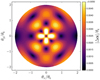Fig. 3. Map of |Δ α(θ)| over a circular grid |θ|≤2 θE for f2 = 0.55, θc = 0.1 θE and γp = 0.1. We set the radius R of the circular region 𝒰 in such a way that the area of 𝒰 is equal to the area of the square grid used in the pure numerical approach, i.e., $R=4{\theta }_{\text{E}}/\sqrt{\pi }\approx 2.257{\theta }_{\text{E}}$. This figure is similar to the Fig. 7 in Unruh et al. (2017) even though it is based on a different approach (see the text for more details). This figure has been obtained with the subpackage spt in less than five minutes for a grid of about 2 × 104 positions.

In Wertz et al. (2018), we analyzed the impact of the SPT on time delays in detail. To achieve this, we compared, for a given lens model, the time delays Δt_ij between image pairs (θ_i, θ_j) of a source β with the time delays Δt̃_ij between the image pairs (θ̃_i, θ̃_j) of the modified source $\widehat{\mathit{\beta }}$ under an SPT. The images θ̃ satisfy the lens equation $\widehat{\mathit{\beta }}=\tilde{\mathit{\theta }}-\tilde{\mathit{\alpha }}(\tilde{\mathit{\theta }})=\tilde{\mathit{\theta }}-\mathbf{\nabla }\tilde{\psi }(\tilde{\mathit{\theta }})$. By construction of ᾶ, we expect θ̃_i to be close to θ, at least in a subregion 𝒰′⊂𝒰 (see Sect. 4 in Wertz et al. 2018). These images θ̃ can be obtained easily thanks to the subpackage lensing. Because its main class Model is designed to accept a user-defined lens model, we benefited from all the tools provided by lensing to characterize the SPT-transformed lens model (see Sect. 4.1). The code below illustrates how to generate the SPT-transformed lensing quantities thanks to the use of the subpackages lensing, sourcemapping, and spt.

5. Impact of the SPT on time delays: Empirical estimation

The first empirical estimation of the impact of the SPT on time delays was presented in Schneider & Sluse (2013, 2014). These authors showed that a quadrupole model composed of a SPL profile predicts the same lensed image positions (with a 0.004 arcsec accuracy) as a composite fiducial model (Hernquist profile + generalized NFW + external shear) for a set of sources $\widehat{\mathit{\beta }}$ and β, respectively¹². We want to stress that the SPL model is not an SPT-generated model from the composite fiducial model but they represent two different models for which the nature of the degeneracy can be approximated by an SPT. Thus, the set of sources $\widehat{\mathit{\beta }}$ was obtained independent of β by fitting the lensed image positions produced by the fiducial model. The top panel of the Fig. 4 in Schneider & Sluse (2014) represents $|\widehat{\mathit{\beta }}|/|\mathit{\beta }|$ as a function of |β|. For sources located in a disk of radius 0.7 arcsec, the connection between $\widehat{\mathit{\beta }}$ and β is slightly anisotropic and roughly resembles a radial stretching of the form Eq. (8) with f₀ = −0.068 and f₂ ≈ 0.012. The bottom panel of the Fig. 4 in Schneider & Sluse (2014) shows that $(\mathrm{\Delta }\widehat{t}/\mathrm{\Delta }t)/(|\widehat{\mathit{\beta }}|/|\mathit{\beta }|)$ were almost constant in the double image regime and not conserved in the quadruple image regime. These authors also found that $(\mathrm{\Delta }\widehat{t}/\mathrm{\Delta }t)/(|\widehat{\mathit{\beta }}|/|\mathit{\beta }|)$ was never smaller than 1.2, reaching a mean of 1.45 for the quadruple image configuration of a source located at |β| ≈0.18 arcsec. Thus, this figure shows that the degeneracy between the SPT and fiducial models can affect the inferred value of H₀ by an average of 20% to up to 45% for particular image configurations.

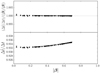Fig. 4. Time delay ratios of image pairs between the composite fiducial model and its SPT-transformed counterpart under a radial stretching with (f0, f2)=(−0.068, 0.012). Top panel: Δt̂/Δt normalized by the ratio $|\widehat{\mathit{\beta }}|/|\mathit{\beta }|$ are very close to 1, even in the quadruple image regime, which disagree with the results obtained in Schneider & Sluse (2014). Bottom panel: The impact of the SPT (cleaned from the pure MST with λ = 1 + f0 = 0.932) is around only a few tenths of percent. The error bars illustrates that the time delay ratios are not conserved in the quadruple image regime, as first suggested in Schneider & Sluse (2014).

As a first application of pySPT, we compare these time delay ratios with those obtained when we transform the fiducial model under a radial stretching Eq. (8) with (f₀, f₂)=(−0.068, 0.012). As shown in Fig. 4, we find that the impact of the SPT on time delays is much smaller than predicted in Fig. 4 in Schneider & Sluse (2014). For instance, they found that a source located at |β|=0.7 arcsec leads to Δt̂/Δt ≈ 1.169 (between the two outer images), whereas we find Δt̂/Δt ≈ 0.935, knowing that the major contribution comes from an MST with λ = 1 + f₀ = 0.932. Moreover, the small anisotropic feature of the empirical source mapping $\widehat{\mathit{\beta }}(\mathit{\beta })$ alone cannot explain this tension.

The discrepancy between our prediction and the results obtained in Schneider & Sluse (2014) are triggered by a minor bug in the public lens modeling code lensmodel (v1.99; Keeton 2001a) that the authors used to compute the time delays. We spotted this bug when we compared the outputs produced with our package pySPT and lensmodel for the deflection angle and deflection potential for the SPL model. Denoting the logarithm slope of the SPL model as a, we found that $2{\widehat{\kappa }}_{\mathtt{lensmodel}}=a{\mathbf{\nabla }}^2{\psi }_{\mathtt{lensmodel}}$ and ${\widehat{\mathit{\alpha }}}_{\mathtt{lensmodel}}=a\mathbf{\nabla }{\psi }_{\mathtt{lensmodel}}$, showing adifferent normalization factor between $\widehat{\kappa },\hspace{0.17em}\widehat{\alpha },\hspace{0.17em}\text{and}\hspace{0.17em}\widehat{\psi }$. This extra normalization factor propagates into the code, leading to a biased value of the time delay Δt̂_lensmodel. It is worth mentioning that, for isothermal profiles (a = 1), this extra normalization factor a has no impact on the lensing quantities computed with lensmodel. This might explain why this minor bug has remained unnoticed so far. Nevertheless, the latter has been fixed and a corrected version of lensmodel has been immediately released by Chuck Keeton. To obtain the Fig. 4 in Schneider & Sluse (2014), the SPL model was characterized by the logarithmic three-dimensional slope γ′=2.24, which is linked to a by the relation a = 3 − γ′, hence a = 0.76 ≠ 1, which finally explains the discrepancy mentioned before.

In Fig. 5, we show the corrected version of the Fig. 4 that we produced with our package pySPT. We confirm that the exact same result can now be obtained from the corrected version of lensmodel. The normalized time delay ratios $(\mathrm{\Delta }\widehat{t}/\mathrm{\Delta }t)/(|\widehat{\mathit{\beta }}|/|\mathit{\beta }|)$ plotted against |β| (top panel) are very close to 1. Thus, the time delay ratios (Δt̂/Δt) (bottom panel) closely resembles the source ratios $|\widehat{\mathit{\beta }}|/|\mathit{\beta }|$ represented in top panel in Fig. 4. This behavior is well understood and is described in detail in the companion paper Wertz et al. (2018). The impact of the SPT (separated from the MST with 1 + f₀ = 0.932) on time delays now reaches only around 0.32% for |β|=0.7 arcsec, which is obviously much smaller than the 20% previously found in Schneider & Sluse (2014). The corrected version now fully agrees with the conclusions drawn from Fig. 4. In addition, this confirms that the degeneracy between the SPT and the fiducial models mimics an SPT, as first established in Unruh et al. (2017).

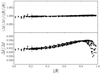Fig. 5. Time delay ratios of image pairs between the composite fiducial model and quadrupole composed of a SPL. This figure constitutes the corrected version of the Fig. 4 published in Sect. 4.3 in SS14. The hat lensing quantities correspond to the SPL model while standard notation is used for the composite fiducial model.

6. Conclusions

In this paper we have presented the pySPT package for analyzing the SPT. The pySPT program relies on several subpackages, the most important of which are lensing to deal with lens model, sourcemapping to define an SPT, and SPT to provide the SPT-transformed lensing quantities defined in previous papers. The subpackage lensing is particular in a sense that it can be used independent of any SPT analysis. To some extent, it somewhat offers a python alternative to the public lens modeling code lensmodel with which it shares a lot of functionalities. The pySPT program implements functionalities for generating lensing quantities produced by SPT-transformed lens models. Thanks to its modularity, pySPT is also designed to accept both user-defined lens model and SPT. In such a case, pySPT constitutes a user friendly interface to deal with the SPT.

As a first application, we used pySPT to explore how a radial stretching may affect the time delay measurements for a fiducial model composed of a Hernquist profile + generalized NFW + external shear. We found that the impact of the SPT is much smaller than first suggested in Schneider & Sluse (2014). We addressed the tension between these results by spotting a minor bug in the public lens modeling code lensmodel that was used by the authors. This bug resulted in biased values of the deflection potential for the nonisothermal SPL model, leading to an overestimated impact of the SPT on the time delays. Using the subpackage lensing, we produced a corrected version of the Fig. 4 published in Schneider & Sluse (2014), which now fully agrees with the results presented in this paper. As a result, the impact of the SPT on time-delay cosmography might not be as crucial as initially suspected. We address this question in details in the companion paper Wertz et al. (2018).

With the next version of pySPT, we plan to include state-of-the-art lens modeling capabilities. For example, combining stellar dynamics data obtained from spectroscopy of the lens galaxy with lensing measurements has become a standard practice within the strong lensing community. Furthermore, we still do not have a clear answer to the question of how the kinematic information of a mass distribution is affected under an SPT. Schneider & Sluse (2013) showed that the fiducial and SPL models discussed in Sect. 5 could not be satisfactorily distinguished thanks to the measurement of the stellar velocity dispersion σP with a typical 10% uncertainty. This thus suggests that the use of σP may be of limited help for breaking the SPT. In a future work, we aim to address this open question with the use of pySPT. In this context, we plan to update the software with a new subpackage fully dedicated to the determination of the stellar velocity dispersion associated with an SPT-modified mass profile. Finally, pySPT is provided not only as an ultimate tool for the lens modeling community, but primarily as an attractive choice to identify the possible degeneracies from which time-delay cosmography may suffer. Nonetheless we hope that its permanent development will attract more users and will extend its purpose to more than just dealing with the SPT.

Acknowledgments

We would like to thank Dominique Sluse and Chuck Keeton for valuable discussions that allowed us to spot and fix the small bug in lensmodel. We are very grateful to the anonymous referee for his comments and suggestions that contributed to improving the quality of pySPT and this paper. This work was supported by the Humboldt Research Fellowship for Postdoctoral Researchers.

References

Appendix A: Generalized pseudo-NFW

To our knowledge, no analytical expression of the deflection potential ψ(θ) for the generalized pseudo-NFW model has ever been published in the literature. For practical purposes, we present such an analytical expression, which has been implemented into pySPT. We first recall that the spherical density distribution ρ(r) of the generalized pseudo-NFW model is defined as (see the Eq. (1) in Muñoz et al. 2001, with n = 3)

$$\begin{array}{c}\hfill \rho (r)=\frac{\rho s}{{(r/rs)}^{\gamma }{[1+{(r/rs)}^2]}^{(3-\gamma )/2}},\end{array}$$(A.1)

where ρs is a characteristic density, rs the scale radius, and γ the logarithmic slope of the density profile at small radius. Up to an additive constant, the axisymmetric deflection potential ψ(θ) is given by

$$\begin{array}{c}\hfill \psi (\mathit{\theta })=r_{\text{s}}{\kappa }_{\text{s}}[\frac{K(0,\frac{3-\gamma }{2};\gamma ;\frac{|\mathit{\theta }|}{\mathit{rs}})-K(1,0;\gamma ;\frac{|\mathit{\theta }|}{\mathit{rs}})}{{\mathrm{\Gamma }}^{\ast }(\gamma /2)}-{\text{Li}}_2(-\frac{{|\mathit{\theta }|}^2}{r_{\text{s}}^2})],\end{array}$$(A.2)

where κ_s = ρ_s r_s/Σ_cr, the term Γ^*(υ)=Γ(υ)/Γ(υ − 1/2) is a particular combination of the gamma function Γ,

$$\begin{array}{c}\hfill K(k_0,l;m;z)={\displaystyle \sum _{k=k_0}^{+\infty }\frac{z^{2(k+l)}}{{(k+l)}^2}{\mathrm{\Gamma }}^{\ast }[k+l+m/2]{}_2{F}_1^{\ast }[k+l,z]},\end{array}$$(A.3)

where ${}_{2}F{}_1^{*}\left[a,z\right]={}_{2}F{}_1\left[a,a,a+1,-z^2\right]$ is a particular Gauss hypergeometric function, and the dilogarithm Li₂(z) can be defined by the series

$$\begin{array}{c}\hfill {\text{Li}}_2(z)={\displaystyle \sum _{k=1}^{+\infty }\frac{z^k}{k^2}·}\end{array}$$(A.4)

Appendix B: Proof of the relation (10)

As a preamble, the notation adopted here differs from that used in Unruh et al. (2017). We use θ as a position in the lens plane and ϑ as the corresponding integration variable for θ. The inverse is partially used in Unruh et al. (2017), in particular in the Sect. 3.3 where ψ̃ and ᾶ are derived.

Starting with Eq. (18) in Unruh et al. (2017), the deflection potential ψ̃ evaluated at the position θ is given by

$$\begin{array}{c}\hfill \tilde{\psi }(\mathit{\theta })=⟨\tilde{\psi }⟩+2{\int }_{\mathcal{U}}H(\mathit{\theta };\mathit{\vartheta })\widehat{\kappa }(\mathit{\vartheta }){\text{d}}^2\vartheta -{\int }_{\partial \mathcal{U}}H(\mathit{\theta };\mathit{\vartheta })\widehat{\mathit{\alpha }}·\mathit{n}\hspace{0.17em}\text{d}s,\end{array}$$(B.1)

where a solution for the Green function H is analytically known when 𝒰 is a disk of radius R

$$\begin{array}{cc}\hfill H(\mathit{\theta };\mathit{\vartheta })& =\frac{1}{4\pi }[ln\left(\frac{{|\mathit{\vartheta }-\mathit{\theta }|}^2}{R^2}\right)+ln(1-\frac{2\mathit{\vartheta }·\mathit{\theta }}{R^2}+\frac{{|\mathit{\vartheta }|}^2{|\mathit{\theta }|}^2}{R^4})]\hfill \\ \hfill & -\frac{{|\mathit{\vartheta }|}^2+{|\mathit{\theta }|}^2}{4\pi R^2}·\hfill \end{array}$$(B.2)

Firstly, we note that |ϑ|=R for all ϑ on the boundary ∂𝒰, which implies

$$\begin{array}{c}\hfill 1-\frac{2\mathit{\vartheta }·\mathit{\theta }}{R^2}+\frac{{|\mathit{\vartheta }|}^2{|\mathit{\theta }|}^2}{R^4}=\frac{{|\mathit{\theta }|}^2}{R^2}-\frac{2\mathit{\vartheta }·\mathit{\theta }}{R^2}+\frac{{|\mathit{\vartheta }|}^2}{R^2}=\frac{{|\mathit{\vartheta }-\mathit{\theta }|}^2}{R^2}·\end{array}$$(B.3)

Thus, the two logarithm-terms in H(θ; ϑ) are equal when we consider the line integral.

Secondly, the term −|θ|²/(4πR ²) in H(θ; ϑ) does not depend on ϑ, and therefore contributes neither to the integral over 𝒰 nor to the line integral. Therefore, Eq. (B.1) contains the term

$$\begin{array}{c}\hfill -\frac{{|\mathit{\theta }|}^2}{4\pi R^2}(2{\int }_{\mathcal{U}}\widehat{\kappa }(\mathit{\vartheta })\hspace{0.17em}{\text{d}}^2\vartheta -{\int }_{\partial \mathcal{U}}\widehat{\mathit{\alpha }}·\mathit{n}\hspace{0.17em}\text{d}s)=0,\end{array}$$(B.4)

where the equality holds because of $2\widehat{\kappa }=\mathbf{\nabla }·\widehat{\mathit{\alpha }}$ and we made use of Gauß divergence theorem. As a result, the term −|θ|²/(4πR ²) in H(θ; ϑ) does not contribute to ψ̃.

Finally, combining Eqs. (B.1), (B.3), and (B.4) leads to the definition of ψ̃ given in Eq. (10). We note that the same reasoning holds for ᾶ, leading to the Eq. (13).

All Tables

All Figures

Fig. 1. Example illustrating some capabilities of the subpackage lensing. Left panel: eight lens profiles with different parameters are combined to generate a complex mass distribution. The total surface mass density is shown in tones of gray and dashed curves highlight few particular iso-density contours. The colored thick curves show the critical curves and the filled and empty markers locate the lensed image positions of two different sources shown in the right panel. The inverted triangles correspond to images of type I (maximum of τ), the diamonds to type II (saddle point of τ), and triangles to type III (maximum of τ). The size of the markers is log-proportional to the magnification of the images. Right panel: the colored lines show the caustics and the two squares locate the sources. The filled (resp. empty) square has seven (resp. nine) images, all shown in the left panel. The axis scale is arcseconds but unit of θE can also be used.

In the text

Fig. 2. Representative example that illustrates how the integration domain 𝒰 is mapped onto the unit disk in the complex plane under a Riemann mapping. Left panel: the color coding depicts the integrand $|\mathit{\vartheta }|\widehat{\kappa }{(\mathit{\vartheta })ln(|\mathit{\vartheta }-\mathit{\theta }|}^2/R^2)$ for all ϑ ∈ 𝒰. It shows a pole at ϑ = θ with θ = ( − 0.5, 0.25) θE and a secondary peak at the origin caused by κ(|ϑ|=0). The lens model is an NIS (θc = 0.1θE) plus external shear (γp = 0.1) transformed by the radial stretching $\widehat{\mathit{\beta }}(\mathit{\beta })=f_0+f_2{|\mathit{\beta }|}^2/(2{\theta }_{\text{E}}^2)$ with (f0, f2)=(0, 0.55). The red circle delimits 𝒰 with radius R. Right panel: integrand after applying the Riemann mapping described in Appendix A in Unruh et al. (2017). The pole ϑ = θ now lies at the origin of the unit (blue) circle of the complex plane. The polar grid (gray lines) allows us to visualize how the Riemann mapping acts on 𝒰. For this figure, we used the subpackage integrals that addresses both the pole and second peak.

In the text

Fig. 3. Map of |Δ α(θ)| over a circular grid |θ|≤2 θE for f2 = 0.55, θc = 0.1 θE and γp = 0.1. We set the radius R of the circular region 𝒰 in such a way that the area of 𝒰 is equal to the area of the square grid used in the pure numerical approach, i.e., $R=4{\theta }_{\text{E}}/\sqrt{\pi }\approx 2.257{\theta }_{\text{E}}$. This figure is similar to the Fig. 7 in Unruh et al. (2017) even though it is based on a different approach (see the text for more details). This figure has been obtained with the subpackage spt in less than five minutes for a grid of about 2 × 104 positions.

In the text

Fig. 4. Time delay ratios of image pairs between the composite fiducial model and its SPT-transformed counterpart under a radial stretching with (f0, f2)=(−0.068, 0.012). Top panel: Δt̂/Δt normalized by the ratio $|\widehat{\mathit{\beta }}|/|\mathit{\beta }|$ are very close to 1, even in the quadruple image regime, which disagree with the results obtained in Schneider & Sluse (2014). Bottom panel: The impact of the SPT (cleaned from the pure MST with λ = 1 + f0 = 0.932) is around only a few tenths of percent. The error bars illustrates that the time delay ratios are not conserved in the quadruple image regime, as first suggested in Schneider & Sluse (2014).

In the text

	Fig. 5. Time delay ratios of image pairs between the composite fiducial model and quadrupole composed of a SPL. This figure constitutes the corrected version of the Fig. 4 published in Sect. 4.3 in SS14. The hat lensing quantities correspond to the SPL model while standard notation is used for the composite fiducial model.
In the text

References

- Bar-Kana, R. 1996, ApJ, 468, 17 [NASA ADS] [CrossRef] [Google Scholar]
- Birrer, S., Amara, A., & Refregier, A. 2016, J. Cosmol. Astropart. Phys., 8, 020 [Google Scholar]
- Falco, E. E., Gorenstein, M. V., & Shapiro, I. I. 1985, ApJ, 289, L1 [Google Scholar]
- Fassnacht, C. D., Gal, R. R., Lubin, L. M., et al. 2006, ApJ, 642, 30 [NASA ADS] [CrossRef] [Google Scholar]
- Hunter, J. D. 2007, Comput. Sci. Eng., 9, 90 [Google Scholar]
- Jones, E., Oliphant, T., Peterson, P., et al. 2001, SciPy: Open Source Scientific Tools for Python, Online; accessed 2017-08-07. [Google Scholar]
- Keeton, C. R. 2001a, ArXiv e-prints [arXiv:astro-ph/0102341]. [Google Scholar]
- Keeton, C. R. 2001b, ArXiv e-prints [arXiv:astro-ph/0102340] [Google Scholar]
- Keeton, C. R. 2003, ApJ, 584, 664 [NASA ADS] [CrossRef] [Google Scholar]
- Muñoz, J. A., Kochanek, C. S., & Keeton, C. R. 2001, ApJ, 558, 657 [NASA ADS] [CrossRef] [Google Scholar]
- Piessens, R., de Doncker-Kapenga, E., Überhuber, C., & Kahaner, D. 1983, QUADPACK: A Subroutine Package for Automatic Integration (Berlin, Heidelberg: Springer-Verlag), 0179 [Google Scholar]
- Press, W. H., Vetterling, W. T., & Flannery, B. P. 1992, Numerical Recipes in C 2nd edn.: The Art of Scientific Computing (Cambridge, UK: Cambridge University Press) [Google Scholar]
- Schneider, P. 2006, in Saas-Fee Advanced Course 33: Gravitational Lensing: Strong, Weak and Micro, eds. G. Meylan, P. Jetzer, P. North, C. S. Kochanek, & J. Wambsganss, 1 [Google Scholar]
- Schneider, P., & Sluse, D. 2013, A&A, 559, A37 [NASA ADS] [CrossRef] [EDP Sciences] [Google Scholar]
- Schneider, P., & Sluse, D. 2014, A&A, 564, A103 [NASA ADS] [CrossRef] [EDP Sciences] [Google Scholar]
- Seljak, U. 1994, ApJ, 436, 509 [NASA ADS] [CrossRef] [Google Scholar]
- Suyu, S. H., Marshall, P. J., Auger, M. W., et al. 2010, ApJ, 711, 201 [NASA ADS] [CrossRef] [Google Scholar]
- Suyu, S. H., Auger, M. W., Hilbert, S., et al. 2013, ApJ, 766, 70 [NASA ADS] [CrossRef] [Google Scholar]
- Treu, T., & Marshall, P. J. 2016, A&ARv, 24, 11 [Google Scholar]
- Unruh, S., Schneider, P., & Sluse, D. 2017, A&A, 601, A77 [NASA ADS] [CrossRef] [EDP Sciences] [Google Scholar]
- Van Der Walt, S., Colbert, S. C., & Varoquaux, G. 2011, Comput. Sci. Eng., 13, 22 [CrossRef] [Google Scholar]
- Watters, A., Ahlstrom, J. C., & Rossum, G. V. 1996, Internet Programming with Python (New York: Henry Holt and Co., Inc.) [Google Scholar]
- Wertz, O., Orthen, B., & Schneider, P. 2018, A&A, 617, A140 [NASA ADS] [CrossRef] [EDP Sciences] [Google Scholar]
- Wilson, G., Aruliah, D. A., Titus Brown, C., et al. 2014, PLOS Biol., 12, e1001745 [CrossRef] [Google Scholar]
- Wong, K. C., Keeton, C. R., Williams, K. A., Momcheva, I. G., & Zabludoff, A. I. 2011, ApJ, 726, 84 [NASA ADS] [CrossRef] [Google Scholar]
- Wong, K. C., Suyu, S. H., Auger, M. W., et al. 2017, MNRAS, 465, 4895 [NASA ADS] [CrossRef] [Google Scholar]