| Issue |
A&A
Volume 618, October 2018
|
|
|---|---|---|
| Article Number | A183 | |
| Number of page(s) | 13 | |
| Section | The Sun | |
| DOI | https://doi.org/10.1051/0004-6361/201832799 | |
| Published online | 01 November 2018 | |
Observational evidence in favor of scale-free evolution of sunspot groups
1
National Research University Higher School of Economics, 20 Myasnitskaya Ulitsa, 101000 Moscow, Russia
e-mail: This email address is being protected from spambots. You need JavaScript enabled to view it.
2
Institut de Physique du Globe, Sorbonne Paris Cité, Paris, France
3
Institute of Earthquake Prediction Theory and Mathematical Geophysics, RAS, Profsoyuznaya 84/32, 117997 Moscow, Russia
Received:
9
February
2018
Accepted:
13
August
2018
Abstract
Context. The hypothesis stating that the distribution of sunspot groups versus their size (φ) follows a power law in the domain of small groups was recently highlighted but rejected in favor of a Weibull distribution.
Aims. In this paper we reconsider this question, and are led to the opposite conclusion.
Methods. We have suggested a new definition of group size, namely the spatio-temporal “volume” (V) obtained as the sum of the observed daily areas instead of a single area associated with each group.
Results. With this new definition of “size”, the width of the power-law part of the distribution φ ∼ 1/Vβ increases from 1.5 to 2.5 orders of magnitude. The exponent β is close to 1. The width of the power-law part and its exponent are stable with respect to the different catalogs and computational procedures used to reduce errors in the data. The observed distribution is not fit adequately by a Weibull distribution.
Conclusions. The existence of a wide 1/V part of the distribution φ suggests that self-organized criticality underlies the generation and evolution of sunspot groups and that the mechanism responsible for it is scale-free over a large range of sizes.
Key words: sunspots / Sun: magnetic fields / methods: data analysis
© ESO 2018
1. Introduction
A power law size-frequency distribution of events gives evidence that the mechanism generating them does not have characteristic sizes. Turbulence is a typical and, at the same time, fundamental example; the distribution of energy versus frequency has a power law part (Kolmogorov 1941). For that reason, a turbulent regime is described by its largest and smallest sizes, whereas characteristic sizes are absent between them. Flicker noise constitutes another example of a well known power law distribution over a range of frequencies (Johnson 1925). This noise is produced by numerous electronic devices. Initially, only distributions with the exponent −1 were linked to flicker noise; later, the notion was extended to power law distributions with different exponents. In practice, (truncated) power law distributions are recorded not only as functions of frequency but (Gutenberg & Richter 1944), landslides (Stark & Hovius 2001), solar flares (Lu & Hamilton 1991; Crosby et al. 1993; Kossobokov et al. 2012), sizes of large cities (Gabaix 1999; Levy 2009), and city fires (Song et al. 2002), but also consumer incomes (Mandelbrot 1960), financial crashes (Mantegna & Stanley 2000), and armed conflicts (Roberts & Turcotte 1998). The density f(x) = 1/xβ of the corresponding distributions has an exponent β that, as a rule, lies inside the interval [1,3]. Processes underlying the cited examples generate a power law distribution as a result of self-organization, since no parameter is tuned.
There is a broad class of systems that tend to a critical state from an arbitrary initial state without parameter tuning. The critical state is characterized by power size-frequency distributions. These systems are referred to as self-organized and critical (SOC). They provide a natural tool to investigate critical phenomena in non-equilibrium processes (Aschwanden 2011; Marković & Gros 2014). A recent review of applications of self-organized criticality to solar physics is given by Aschwanden et al. (2016). The first SOC model, introduced by Bak et al. (1987), quickly spread into different fields. This model describes the evolution of a system under continuous loading. Sometimes the system becomes locally overloaded; overloading triggers avalanches that conservatively transport stress through the system from the overloaded region to the boundary where dissipation occurs. The concept of slow loading and quick redistribution of this load with stress release at the boundary underlies numerous modifications of the initial model. Isotropic models constructed on a square lattice are characterized by power size-frequency distributions of avalanches with exponents β ∈ (1,2); see Shapoval & Shnirman (2005). To our knowledge, the exponent β = 1 has not been reported in the models considered so far.
When a truncated power law distribution has been identified, one builds a power law over a range of scales and estimates the relevant exponent. The disagreement between the observed distribution and the identified power law at large scales is attributed to a finite size effect. Researchers identify two parts in empirical distributions, that is, a power law segment on the “left” (i.e., small sizes) and a bend down on the “right” (i.e., larger sizes). Others question the existence of these two parts and propose that a single law underlies the observations. Using parametric or non-parametric estimates, they propose what they find to be sufficiently accurate approximations with log-normal, Weibull, or other distributions (Boffetta et al. 1999; Eeckhout 2004, 2009; Dragulescu & Yakovenko 2001).
Such a discussion is relevant to the study of the distri-bution of sunspot groups versus their sizes (Bogdan et al. 1988; Baumann & Solanki 2005; Jiang et al. 2011; Muñoz-Jaramillo et al. 2015). This paper discusses properties of the sunspot groups instead of separate spots because databases listing sizes and coordinates on a daily basis only give information on groups. The support of the distribution covers approximately four orders of magnitude ([1,104]). It can be split roughly into two parts. The left part (describing small groups) admits a power fit (Jiang et al. 2011). The faster decrease of the right part (larger sizes) is well represented by a log-normal distribution (Bogdan et al. 1988; Baumann & Solanki 2005; Jiang et al. 2011).
The accuracy of information relevant to small groups needs clarification. Narrowing the approximation interval by eliminating smaller groups, one can get a good fit to the group distribution with a single log-normal distribution. Muñoz-Jaramillo et al. (2015) eliminate a left interval of available (i.e., smaller) sizes, which extends over one order of magnitude, and compare log-normal, power, and Weibull fits to remaining data by standard statistical methods. They conclude that the quick decrease of the right part of the distribution (i.e., larger sizes) is closer to a log-normal function, but that a Weibull approximation becomes more accurate if the left part of the distribution is included in the interval under consideration. Looking for the best fit with a composite distribution, Muñoz-Jaramillo et al. (2015) combine Weibull (at the left) and log-normal (at the right) distributions. Nevertheless, it is fair to say that the comparison of composite distributions against single laws has not yet been fully worked out.
Although the general pattern of the above discussion is clear, the diversity of conclusions is in part due to uncertainties on the detail of issues such as processing different databases; fitting only part of the observed size interval; applying a variety of statistical methods; the fact that only half of the Sun is available for observations (see Sect. 3.2); the ambiguity in the definition of sizes versus which the distribution is constructed (see Sect. 2).
In fact, when solving the approximation problem with complex errors in databases, the authors cited above rely on different samples and use non-unified methods for comparing the best solutions. Muñoz-Jaramillo et al. (2015) have recently achieved a significant step forward in the unification of data processing by considering jointly all available databases and introducing a universal statistical procedure to fit the distributions.
According to Chapman et al. (1997), the total magnetic flux of the group is approximated rather accurately by a linear function of the area of the active region (which consists of sunspot and plage areas). Therefore, regularities found in the size-frequency distribution of the groups could also be valid for fluxes and other magnetic structures observed on the surface of the Sun. For example, Muñoz-Jaramillo et al. (2015) report that a Weibull distribution agrees not only with the distribution of spot groups but also with that of other magnetic structures. The universality of their Weibull approximation would seem to provide by itself convincing evidence for its correctness. However, the conclusions of previous papers on the distribution of magnetic structures are somewhat controversial. Other authors advocate log-normal (Zhang et al. 2010; Schad & Penn 2010), Weibull (Parnell 2002), and truncated power (Meunier 2003; Zharkov et al. 2005; Parnell et al. 2009) approximations to these same distributions. Therefore, generalization of results concerning different magnetic structures to the distribution of the groups is not straightforward.
The question of the best approximation is also linked to the invisibility from the Earth of those groups that lie on the “back” side of the Sun. Some groups become visible from the Earth some time after having appeared on the Sun; other groups rotate with the Sun away from sight and cease to be observed from the Earth. There are also groups that are not observed at all from the Earth. We apply a sorting of groups prior to the estimation of size distribution such that (observed) groups used for the estimation constitute approximately half of the groups that have actually appeared on the whole Sun (Sect. 3).
The size of spot groups can be defined in various ways. One can simply pick up all areas given in a catalog and construct an empirical distribution f1 from this sample; f1 shows the distribution of the areas observed on any day in the catalog. It is called the snapshot distribution. This distribution is convenient because its construction does not require any sorting. On the other hand, if a group is recorded over n days in the catalog, the n areas are used separately when f1 is constructed. Therefore f1, in general, does not represent the genuine distribution of groups. The size of a group could be defined in such a way that each group is given a single size; the maximal area associated with the group in a catalog is an example of such a measure of size. The corresponding group distribution, f2, in general differs from f1 and depends on the sorting process. The construction of a correct size-frequency distribution of the groups needs a unified sorting method. We solve the “invisibility problem” by removing groups for which the location of the maximum is unknown.
Rather than presenting an analysis of distributions f1 and f2, this paper introduces a new characteristic of spot groups, namely the sum of recorded areas that can be interpreted as a (space × time or spatio-temporal) volume of groups and is referred to below as a size. Introducing size is standard practice in models of self-organized criticality. The change from areas to sizes (volumes) enlarges the support of the distribution by one order of magnitude approximately (i.e., ten times). We find that the power law segment of the distribution is also extended by up to two or three orders of magnitude. The exponent of the power law segment is close to one. A bump and an abrupt turn down to the right follow the power law segment: we show that such a transition from a power function to a quick bend down does not fit a Weibull distribution. The best fits and their parameters are estimated by the maximum likelihood method applied to the datasets themselves, whereas figures illustrate probability density functions that are preliminary binned over intervals whose length is chosen with an exponential step. Our findings are stable with respect to the sorting procedure and choice of catalogs. Based on these results, we conclude that the mechanism generating (small and medium sized) spot groups is scale-free.
The paper is organized as follows. In Sect. 2 we describe databases and summarize the area-frequency relation discussed in several papers mentioned above. We present our findings in the next Sections. The size of the groups is introduced in Sect. 3. Further, in Sect. 3 we introduce the required sorting tools, construct the size-frequency relation, and exhibit the power law segment. To verify the stability of this power law segment, we introduce in Sect. 3.4 an extrapolation of the sizes for those groups that leave the visibility range as they rotate with the Sun. In Sect. 3, we also show that a Weibull distribution does not fit the observations. Section 4 relates our finding to other studies. Section 5 concludes. All technical details are moved to the Appendices.
2. Area-frequency relationship
2.1. Catalogs
Four available free catalogs contain daily records of sunspot groups. The first catalog (1874–1975) has been compiled by the Royal Greenwich Observatory (RGO). It contains information about 29 800 groups in 161 413 records. Each record is represented by a line in a computer file which contains the results of observations. From 1976 onwards, a catalog in the RGO format is supplied by the US Air Force. The data is collected by the Solar Observing Optical Network (SOON); the catalog contains information about 7421 groups in 80 106 records (those up to the end of 2013 are used in this paper).
Two other catalogs rely on observations made in Pulkovo, Saint–Petersburg region, Russia (Pulkovo’s Catalog of Solar Activity, PCSA, 1932–1991) and in Kislovodsk, Russia (Kislovodsk Mountain Astronomical Station, KMAS, Tlatov et al. 2016; see Table 1).
“Corrected whole spot areas” are given in millionths of solar hemisphere (μH) by catalogs RGO, SOON, and KMAS. The PCSA catalog gives a single value of the area, called the group area; it is also measured in millionths of solar hemisphere.
Catalogs of sunspots and sunspot groups give their Carrington longitudes lS relative to the Sun, on the whole interval [0°, 360°], at the time of first appearance on the visible hemisphere of the Sun. We restore these observations to the longitudes that refer to the west limb on the visible hemisphere. The range of these visible longitudes lE is close to [0°, 180°]. The Carrington longitudes lS are transformed into the coordinates lE associated with Earth observers by a simple linear shift (modulo 360; as, according to Royal Greenwich Observatory (1980), “it should be noted that longitudes are based on the ephemeris given in the Astronomical Ephemeris, assuming a solar rotation period constant at all latitudes”). With this shift, any point rotating with the Sun increases its longitude lE each day by 360/T (modulo 360), where T = 27.2753 is the estimate of the Sun’s (synodic) rotation period at a reference latitude. This transformation is basically the inverse of the procedure followed by the original observers. We note that the differential rotation of the Sun does not intervene in the transformation; indeed, this transformation involves the reference latitude that corresponds to the exact Carrington rotation period.
Number of records and groups in the databases.
2.2. Graphs and uncertainty
We start from a visual analysis of the size-frequency relationship. Corresponding graphs are given in double–logarithmic coordinates (where power functions are transformed into straight lines). The widths of horizontal bins are chosen with an exponential step. To avoid introducing a new term, we call the distributions obtained with these increasing width of bins interval probability functions ipf) φ; the value φ(x) is the fraction of the sample elements the size of which belongs to the interval [x/c, xc), where c > 1 is some constant. The choice of an empirical ipf instead of a classical probability density function (pdf) reduces the noise in the right hand part of the graphs, which is often essential for the identification of the distribution’s power law range. If the pdf is a power function, so is the ipf, and its exponent is smaller than that of the pdf by one unit. (1/xβ−1 vs. 1/xβ; see Appendix A). Since the presence of a horizontal part in the graph can be ascertained “with a naked eye”, one can immediately distinguish visually a 1/x part of the distribution with the ipf representation of the data, as 1/x is transformed into a horizontal segment of the ipf. When comparing observations with theoretical random variables, one has to construct the ipf of both theoretical and empirical distributions.
Figure 1 illustrates the problem of the best fit. It exhibits the empirical ipf computed from the RGO catalog for the snapshot distribution and two distributions of groups versus their maximal areas. One of those two distributions (max1 in Fig. 1) is constructed from all the groups, whereas the second distribution (max2) comes only from groups that achieve their maximal area deeply inside the range of visible longitudes (following (Baumann & Solanki 2005), we chose a 60° interval centered on longitude 90°). The corresponding complement cumulative distribution functions are shown in Appendix E.
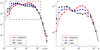 |
Fig. 1. Left panel: interval probability function, ipf, φ(A) = ProbA/c ≤ area < Ac, c2 = 1.5, found with the RGO database for all groups observed on any day (snapshot distribution), for maximal observed areas of all groups (max1), and for those whose maximal area is observed at longitudes lE ∈ [60,120] in coordinates associated with Earth observers (max2). Right panel: enlargement of the rectangular window in left part of the figure ( μH are millionths of a solar hemisphere). |
Figure 1 illustrates many of the remarks made in the Introduction. All graphs shown in Fig. 1 present a (flat) quasi-power law segment which extends over less than two orders of magnitude. Their slopes are slightly positive for the snapshot distribution (red line in Fig. 1; interval [5, 200] hundred millionths of solar hemisphere (μH)), and slightly negative for the other two graphs (on interval [7,300] μH for the blue curve and [8, 500] μH for the black curve). After elimination of the first points at left, the shape of all the three graphs can be naturally fit by a composite distribution which is interpreted as a power-law section at the left and a log-normal section at the right by Jiang et al. (2011), or as a Weibull distribution by Muñoz-Jaramillo et al. (2015). These fits agree with each other because the Weibull distribution is similar to a power function when the argument is small, and decreases exponentially later. We do not enter into the details of fitting the full graph, but highlight the question: do the graphs represent a single or a two-piece distribution? We recall that the latter choice agrees with the hypothesis of a scale-free left part of the distribution.
3. Size-frequency relationship
3.1. Sizes instead of areas
Let G0 be an investigated set of sunspot groups. Each catalog is characterized by its own G0. For any group g ∈ G0 observed on days t1, . . ., tn, n depending on g, the sequence of the group’s areas A1, . . ., An is recorded in the catalog. V = V(g) is the sum of all the recorded areas (measured in μH) of the group g; we will call it the size of the group g. This size is interpreted as a spatio-temporal volume. The distribution of groups versus size, that is, the size-frequency relationship is shown in Fig. 2 (i.e., the empirical ipf of the set G0, denoted by φ0).
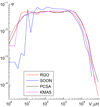 |
Fig. 2. ipf φ0(V) = Prob{V/c ≤ size < Vc} of the group sizes for the sets G0 of catalogs RGO (28 points in the graph), SOON (26 points), PCSA (28 points), and KMAS (27 points); c2 = 1.5; V is measured in μH. |
In Fig. 2 we see that for all four catalogs, the graphs of functions φ are close to power functions with exponents of approximately zero over at least the interval [10,2000], that is, over two orders of magnitude. Comparing Fig. 2 with 1, we see that the length of the power law segments has increased by approximately one order of magnitude. To the right of the power law segments, the graphs abruptly bend down in Fig. 2.
Since only half of the Sun is visible from the Earth and the solar rotation period is approximately 27 days, the catalogs contain at most 14 successive observations of a given group. The genuine sizes of the groups that come into the visibility range from the back side of the Sun or leave it for this back side are not known, so that the fate of part of the group sizes, on which Fig. 2 is based, is uncertain (see Sects. 3.2 and 3.3). We now examine how this uncertainty affects the power law in the left part of the graph in Fig. 2 and the value of its exponent. We also introduce an extrapolation procedure that corrects the size of outgoing groups (Sect. 3.4).
Some groups, which live longer than a solar rotation period, return to the visibility range of longitudes. They are labeled as new groups in the catalogs. Presumably, the number of such groups is small and the majority have too large a size to lie on the power law segment. Therefore we ignore the error they generate.
3.2. Preliminary sorting at the right boundary of the visibility range.
Imagine an observer who studies the back side of the Sun. He observes precisely those longitudes that an Earth observer cannot see. A simple grouping of the samples collected by the two observers does not solve the invisibility problem because the spots leaving the observers are seen and recorded by both of them. In order to escape double records, the observers can identify and remove the sunspot groups that leave the visibility range while attaining their maximal area on the last day of observations. With such a preliminary sorting, the Earth observer records approximately half of all groups that have appeared on the (visible and invisible sides of the) Sun. The other half of the groups is recorded by the imaginary observer.
There are numerous possibilities to segregate groups between Earth and imaginary observers. Our preliminary sorting has clear advantages. Firstly, it contains all groups whose maximal area lies within the visibility range. From now on we assume that the observed local maximum of the area (in the sequence of the recorded areas) is also the global maximum. As remarked in the Introduction, the distribution of the groups versus their maximal areas have been investigated by many authors, for example, by Baumann & Solanki (2005) and Muñoz-Jaramillo et al. (2015). Therefore our approach, dealing with all the groups whose maximal area is recorded, is directly comparable with other studies. Secondly, the above operation provides a simple evaluation of the size of those groups that leave the visibility range (see Sect. 3.4).
By G1 we denote the set of group areas that remain after the preliminary sorting just discussed. Formally,
 (1)
(1)
where Ai = Ai(g) is the area of group g ∈ G0 on the ith day of observations; index n(g) indicates the last record of the group g in the catalog. The ipf found for the distribution of the group sizes of the set G1 is denoted by φ1.
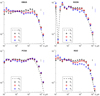 |
Fig. 3. Segments of the size-frequency relations for catalogs RGO, SOON, PCSA, KMAS: ipf φ0 (constructed with set G0), φ1, φ2 (constructed with G1), and φ3 (constructed with G3); c2 = 1.5; vertical (black and blue) lines indicate the 0.95-confidence intervals computed for φ1 and φ3 at point V ≈ 500. V is measured in μH. |
3.3. Identification problem at the left visibility boundary
Some of the groups that appear at the left visibility boundary were “born” on the back side of the Sun. Their first recording thus does not correspond to their “birthday” but to a later day. In order to actually include in our sampling half of the groups that have appeared on the entire Sun, we have included in our process all groups that were first noticed at the left limb of the Sun and are growing, no matter whether they have just been born or were born before and rotated with the Sun into view. On the other hand, groups first noticed at the left limb of the Sun that were born on the back side and are decreasing should be disregarded (as they would have been processed by the imaginary observer). However, it is impossible to distinguish individually between these groups and those groups born exactly at the left visibility boundary, even if the first recorded area is large, since groups may quickly attain their maximal area (in just one or two days) and then slowly decrease (McIntosh 1981). In order to distinguish between the two types of groups, observations at smaller longitudes l (l < 0) would be required.
We could then assign a number ν ∈ [0,1] to each incoming group which estimates the probability that this group was not born before being recorded for the first time. We have assumed that the first longitudes (between 0 and some positive ltest) are invisible and re-formulate the identification problem for the groups recorded close to the new left boundary longitude ltest. Since records concerning longitudes from the [0, ltest] interval are, in fact, available, we can count the number N+ of the groups born at the new boundary ltest as well as the number N− of the groups born earlier but still observed to the right (east) of ltest. Then N+/(N+ + N−) is an estimate of the probability ν that a group observed at the left visibility boundary has just been born.
This procedure is insensitive to the size of groups. However, small groups rather than large ones are likely to be just born. Therefore, the observable range of the group sizes is split into mutually non-overlapping intervals J1, J2, . . .. The above procedure, namely the computation of N+, N−, and ν, is applied to each interval J separately (see details in Appendix C). The test longitude is chosen as ltest = 30°. As a result, each group g observed at the left visibility boundary is assigned a number ν = N+/(N+ + N−) ∈ [0,1], which is an estimate of the probability that g has just been born. The other groups from G1 are assigned ν = 1.
The construction of the ipf requires the computation of the number of elements with a given size. If ν(g) is assigned to a group g, then this element g has to be counted with probability ν(g) when computing the ipf. In other words, the average contribution of g to the number of groups is equal to ν(g).
More rigorously, we have defined the interval probability function φ2 describing the distribution of the recognized groups in the following way. Let I(x) = [x/c, xc] be one of the bins used in the construction of the size-frequency relation. For each group g with the size V(g), we say that the indicator σ(V, I(x)) = 1 if V ∈ I(x). Otherwise, σ(V, I(x)) = 0. Then
 (2)
(2)
Instead of assigning probabilities ν to incoming groups, one can eliminate all the groups that achieve their maximal area at the left visibility boundary. In terms of probabilities ν, it means that all these incoming groups are given the probabilities ν = 0. The set constructed in this way and the corresponding ipf are denoted G3 and φ3 respectively. It is worth noting that ipf φ2 is constructed from the set G1 (Formula (1); no G2 is used in this paper). In Table 1 we report the number of groups in the sets G0, G1, and G3.
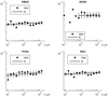 |
Fig. 4. Segments of the size-frequency relations for catalogs RGO, SOON, PCSA, KMAS: ipf φ1 (circles) are shown together with theoretical values calculated for the power law distribution on the interval [a,b], where [a,b] is [10, 1000], [100, 1000], [10, 1000], [10, 1000] for RGO, SOON, PCSA, and KMAS respectively and with 0.95-confidence intervals illustrated by vertical lines; c2 = 1.5. V is measured in μH. |
According to Fig. 3, the identification procedure only weakly affects the width of the power law segments and their exponents. All ipf still have an almost horizontal part that extends over more than two orders of magnitudes. The power law segment is sometimes followed by a small upward bump and then, to its right, by an abrupt bend down. The ipf s for the KMAS, PCSA and RGO catalogs display very similar patterns. The ipf s φ1 constructed from the SOON catalog deviate from that pattern; the existence of the bump is questionable, and instabilities occur for smaller values of size V.
We next computed the best approximation to the empirical probability density function from the set G1 using the maximum likelihood estimation (MLE), and constructed the corresponding ipf. Figure 4 displays this ipf and its 0.95% error bars together with ipf φ1. We stress that MLE is applied to the set G1 without any binning; Fig. 4 displays the ipf for convenience. The observed values (full dots) are mostly within the error bars of the best (MLE) approximation to their distribution. The agreement between the theoretical approximation and the values of φ1 is better in the domain of larger groups (i.e., at the right part of the graph). We note that the pattern of the oscillations exhibited by the four graphs has much in common. The mutual correlations ρ between the six left points of the curves representing KMAS, PCSA, and RGO are ρ(KMAS, PCSA) = 0.85, ρ(PCSA, RGO) = 0.44, ρ(RGO, KMAS) = 0.76. The SOON curve is excluded because of its large oscillations at the left part of the graph. This similarity in the patterns and the large values of the correlation coefficient support the hypothesis that values reported in these catalogs are subject to identical procedures and errors (likely rounding off). These common errors generate a specific noise that decreases from the left to the right.
Despite this noise, we performed a chi-square goodness of fit test. The null hypothesis specifies that the observations are consistent with the power law over a given range [a, b] of the sizes. The right boundary b is fixed to 2000 μH, which corresponds to the right end of the power law segment observed in Fig. 3. The test is run with different values of the left boundary a located between 50 and 300 μH. The data is split into nmax bins [an, an+1], n = 1, 2, . . ., nmax, a1 = a, anmax + 1 = b,  is fixed to a constant. Computing the χ2-statistics for all four catalogs, we plot the χ2-probability (i.e., the corresponding p-value) as a function of a in Fig. 5a. The p-value indicates the probability of observing the database (or a more extreme set), given that the true distribution function is power law. The test internally determines the exponent of the power law. The test values found with databases RGO, KMAS, PCSA, and SOON respectively are shown in Fig. 5b as a function of a. When a increases from 50 to 300, the volume of the samples varies from 11203 down to 5576 (RGO database), from 7836 to 4103 (KMAS), from 6920 to 3420 (PCSA), and from 5782 to 2801 (SOON). Figure 5 represents the result of the test with the bin length c = 1.2 and the number nmax of the bins decreasing from 25 to 16. We note that the MLE method, discussed earlier and resulted in Fig. 4, more accurately assesses the exponent of the power law, but new estimates are also located in a neighborhood of one.
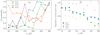 |
Fig. 5. χ2-probability (panel a) and the exponent (panel b) of the power law distribution versus the left boundary of the power law interval; 2000 is assigned to the right boundary; the logarithmic length of the bins is c = 1.2; The smallest values of the PCSA curve are 0.006 and 0.002. |
The most of the χ2-probabilities found with all four catalogs are greater than 0.1. These probabilities tend to be larger at the right than at the left, which is in line with the reduction of noise of the ipf from the left to the right. Thus, the goodness of fit test does not reject the hypothesis that the distribution of the sunspot groups exhibits a power law part. The length of this part is approximately 1.5 orders of magnitude minimum. The binning reduces noise and makes the observed and theoretical distributions closer. The power law segment is transformed into a quick decay to the right of V = 2000 μH; see Fig. 3. On the contrary, to the left of the interval [50, 300] μH, the power law is still observed (Fig. 3), but a high noise level means we cannot reject the null hypothesis that the distributions are similar. Lower values of the χ2-probability on larger segments are expected.
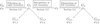 |
Fig. 6. Verification procedures applied successively: sorting of the outgoing groups, identification and elimination of incoming groups, and subdivision of the sets G1 and G3 into subsets to check the stability of the observed power law segments (see text). |
This concludes the stability check announced in Sect. 3.1: starting from the power law segment in the size-frequency relation φ0 (Fig. 2) constructed from the given set G0 of all recorded groups, we have checked the stability of the conclusions concerning the width and exponent of the power law segment in two ways (Fig. 6): first, with the preliminary sorting, we have eliminated the outgoing groups that have not attained their maximal area, resulting in ipf φ1 (Sect. 3.2); second, we identify in a probabilistic way the incoming groups, resulting in the interval probability functions φ2 and φ3 (Sect. 3.3). We find that neither the width of the power law segment nor its exponent, are influenced, despite the fact that the number of groups that are affected by these sorting methods is not small (Table 1).
We continued to check the accuracy in the computation of the exponent β, completing the plan given schematically in Fig. 6. We separated the set G1 (defined by Formula (1)) into two subsets such that two successively recorded groups with similar sizes are put into different subsets 1 or 2, G1,1 and G1,2, which contain approximately the same number of groups (see details in Appendix D). Our idea is to work with two weakly dependent samples with similar statistical properties and check the equality of the exponents β computed from each sample. By the maximum likelihood method (discussed in Appendix B and applied directly to the corresponding samples without any preliminary binning) we find the truncated power law distributions that fit the subsamples the most accurately. The computed exponents of the power functions are denoted β1,1 and β1,2. In the same way, the exponents β3,1 and β3,2 are computed with the set G3.
Exponents of the best fits α/Vβ to the empirical probability density functions.
Prior to the identification procedure, the exponent β is approximately 1 for RGO, SOON, and PCSA, and less than 1 for KMAS, Table 2. After identification, β is very stable and still within less than 1% from 1 for PCSA. The exponent varies more for the other catalogs and can reach 1.08 for KMAS and 1.15 for RGO and SOON. The order of magnitude of the exponents β shown in Table 2 can be roughly summarized by their average, equal to 1.02, thus within 2% of 1 (this value, given for indicative purposes only, is not a rigorous mean value).
3.4. Volume correction
In addition to the question raised in Sect. 3.3, the catalogs provide incomplete information regarding the sizes of the groups from the set G1 that leave the visibility range as the Sun rotates: when these groups attain the back side of the Sun, their areas are not known. We estimated these unknown areas by extrapolating the observed areas in the following way. We introduced two simple extrapolations based on the last observed and maximal areas. The first extrapolation is linear with respect to the observed areas, whereas the second is linear with respect to the square root of the areas. Both operations are mathematically well defined: they allow us to assign a finite size to all groups g ∈ G1 because they attain the maximal area before the last day of observation (see definition (1) of G1). The extrapolation is required for 2773 out of 25 565 groups of G1 for catalog RGO; 611 out of 9 938 groups for catalog SOON; 128 out of 15 523 groups for catalog PSCA; 2462 out of 17 076 groups for catalog KMAS. Those extrapolations are in line with the discussion regarding the decrease of group size with time (Petrovay & Moreno-Insertis 1997; Martinez Pillet et al. 1993; Petrovay & van Driel-Gesztelyi 1997).
Group records relevant to days t1, t2, . . ., tn can contain gaps: for some rare i the difference ti+1 − ti ≠ 1. We interpolated these gaps using areas Ai and Ai+1 associated with ti and ti+1. We applied two linear interpolations, linear either with respect to the group area or to its square root.
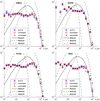 |
Fig. 7. ipf of sizes (φ3, ×-marked graph) and corrected sizes obtained by linear extrapolation and interpolation with respect to areas (φr,a, plus-marked graph), and with respect to the square root of area respectively (φr,l, circle-marked graph). Best fits with Weibull distributions computed on the intervals [10, +∞), [100, +∞), and [10,1000) are given as ipf with solid, dashed, and dash-dotted lines respectively; c2 = 1.5. V is measured in μH. |
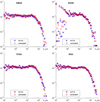 |
Fig. 8. ipf of sizes (φ3, ×-marked graph) and corrected sizes obtained by linear extrapolations with respect to the square root of areas (φ3,l, circle-marked graph); c2 = 1.1. |
The interval probability functions constructed with the linear extrapolation and interpolation with respect to the areas is denoted by φr,a. When the extrapolations and interpolations are linear with respect to the square root of the area, the ipf is denoted by φr,l. Figure gives evidence that the power law segments of the ipf for the group distribution versus the corrected sizes are almost identical to each other and to those of φ3 constructed with unrevised sizes.
The ipf for the distribution of the corrected sizes using smaller bins is given in Fig. 8. Markers are too close in the graph to show three curves; therefore, we have presented the distribution obtained by linear extrapolation and interpolation with respect to the square root of the areas and the distribution of the unrevised sizes. The latter serves as a point of reference. We observe that the power law segment is clearly present in Fig. 8 and hardly affected by the correction.
Finally, we attempted to determine whether any Weibull distribution gives a good fit to the observations, using the maximum likelihood method (Appendix B). The ipf of these distributions are shown in Fig. 7. We stress that Fig. 7 exhibits merely the ipf of the distributions (not a probability density or a cumulative distribution function). Clearly, the ipf s of the Weibull approximations cannot simultaneously fit the power and the exponential parts of the graphs and impose at the same time that the area under them be normalized to 1.
A more complete examination reveals that the parameters of the best log-normal and Weibull fits to the size-frequency relationship are sensitive to the choice of the approximation interval (on which the fit is computed). On the contrary, the exponent of the power law varies only slightly under such changes. This observation favors a power law distribution over a Weibull distribution.
4. Discussion
We show that the distribution of sunspot groups versus their sizes exhibits a 1/xβ power law segment that extends over more than two orders of magnitudes. The exponent β is very close to one. To the right of this power law segment the distribution falls off much more quickly. We have obtained this empirical distribution by introducing a new definition of the size of a group, namely the sum of all its daily areas recorded in a given catalog. By considering sizes instead of areas themselves, we extend the range of the power law segment by more than one order of magnitude.
Another hypothesis, that of a single distribution, competes with that of a splitting of the distribution into two parts. This has been tested by Muñoz-Jaramillo et al. (2015) with a Weibull distribution that has a quasi-power law segment on its left part and an exponential segment on the right part. These authors accurately fit the area-frequency relation of sunspot groups by such a distribution over the range of areas A > 10 (A > 100 for the SOON catalog). A Weibull probability density fits the observations in this case because the change from sizes to areas (1) alters the exponent of the quasi-power law segment and (2) reduces its length on 1-1.5 orders of magnitude. However, a Weibull distribution does not yield an adequate fit to the size-frequency relation (Sect. 3): it may fit a ∼ 1/x segment on the left, but it changes from a power law to an exponential decay much more slowly than the observed size-frequency relationship does (see Sect. 3).
Here we discuss the difference of the observed distribution from a log-normal one. Following the representation of the power law: ln f ∼ –β ln x, the log-normal probability density f(x) can be written in a form  , where β and σ are the two parameters of the distribution. The factor
  represents β but this “exponent” varies with x. Its increase implies that the log-normal probability density can look like a power function in the log-log scale but exhibits concavity. The ipf of the log-normal probability density inherits this property. However, the exponent of the observed ipfs is not an increasing function, in the range [10,3 × 10³] μH, Figs. 3, 4, and 7. This favors a power law over the log-normality in this range.
The right end of the power law segment corresponds to the groups whose area is several hundred millionths of solar hemisphere (μH) and, therefore, the size is several thousand millionths of solar hemisphere. The latter corresponds to the linear size of supergranules (Rieutord & Rincon 2010). Supergranulation likely determines an upper characteristic size of solar magnetic structures, and the power law segment extends up to this characteristic size. In the SOC models, the largest events occur more rarely than the power law predicts. This insufficient occurrence is typically explained by a finite size effect. If the supergranules appear through collective interactions of smaller magnetic features (Rieutord& Rincon 2010), exceptionally large interaction may be required to result in the appearance of a supergranule.
We emphasize once again that catalog records are subject to errors. Weather conditions reduce visibility, distorting the data and leading to gaps; the discrete nature of observations shortens the maximal areas of the groups recorded in the catalogs. The underestimation of areas is discussed in Royal Greenwich Observatory (1980), and some efforts are focused on the improvement of databases (Willis et al. 2016; Svalgaard & Schatten 2016; Usoskin et al. 2016); however all these studies do not report areas of individual groups required for our research. In our opinion, the effect of the bias is small. Other errors arise from the invisibility of the back side of the Sun (discussed in Sects. 3.2 and 3.3) and data processing. The transition from areas to sizes can increase inaccuracy. To mitigate errors, we have introduced adjustment procedures, namely (i) interpolation that closes up gaps (Sect. 3.4), (ii) extrapolation of the areas of outgoing groups to make their sizes more precise (Sect. 3.4), and (iii) a procedure of identification of incoming groups (Sect. 3.3). An important result is that the length of the power-law segment and its exponent β remain stable after implementation of all these procedures.
Our method for identifying incoming groups appears to be new: we derived statistically adequate conclusions by dealing with a half of the groups appeared on the Sun, namely those that are born on the visible part of solar limb. When attempting to deal with the invisibility of a half of the Sun, earlier researchers identified only long-lived spots (Henwood et al. 2010) or neglected groups that were observed close to the edges of the solar limb (see, e.g., Baumann & Solanki 2005).
Four available catalogs (RGO, SOON, PCSA, KMAS) were used in our study. Each catalog is relative to a single station. Records collected on the same day at different stations differ, in general, from one another. In particular, the recording of small spots (less than 100 μH) at SOON undoubtedly differs from their recording at the other stations (Figs. 2 and 8). Large oscillations of the ipf associated with small changes in sizes of groups could be linked to rounding off (some last digit of values appear more frequently than others). Larger values of the exponent β obtained from SOON could be due to more accurate registration of small areas (due to better weather conditions, specific devices, etc). Indeed, a more accurate registration (i) increases the number of small events at the expense of tiny groups that are not visible in the other stations; (ii) increases the size of groups, whence decreasing the relative number of moderate events. Nevertheless, the better visibility of sunspot groups achieved at SOON superimposed on a specific treatment of the observations magnifies the variance of the ipf in the range of small values. Therefore, better observational instruments do not provide a more accurate empirical power law.
Parnell et al. (2009) discuss in details how self–similarity of small-scale magnetic fluxes arises. Their main suggestion is that the behavior of the magnetic field on the surface of the Sun is dominated by a continuous convective motion of plasma; new flux bundles emerge, coalesce, become fragmented, and annihilate (Schrijver et al. 1997). The total resulting flux of emerged magnetic structures is zero. These magnetic structures of both polarities can encounter other magnetic structures during their evolution; flux bundles coalesce if their polarities are identical, cancel in the opposite case. The breakdown of magnetic structures eventually leads to their fragmentation. Such evolution of flux bundles in the convective zone corresponds to a spatial redistribution of energy, similar to the evolution of sand-pile models. Nevertheless, modeling of the self-organization of sunspots in the framework of the solar dynamo theory still remains a puzzle for researchers. Uritsky & Pudovkin (1998) give arguments supporting SOC of magnetic structures on the Sun, investigating the geomagnetic AE-index and considering power law distributions of frequencies, not sizes. We emphasize that in models describing SOC, the size-frequency relationship is usually investigated for spatio-temporal volumes, as we have done here, whereas individual areas are rarely referred to. Thus, when associating the sizes of sunspot groups with their “volumes”, we remain in line with approaches to SOC.
Researchers have already found power laws in the size-frequency distribution of solar magnetic structures, but with exponents from the range [−2, −1.5]. For example, Parnell et al. (2009) claim that the probability density of solar magnetic fluxes – understood as the surface integral of the normal component of the magnetic field – follows the power law 1/x−β with the exponent β ≈ 1.85. This β clearly differs from 1 found in this research. There are reasons for the difference between these exponents. Parnell et al. (2009) study solar magnetic features, whose flux lie within the range of [1016, 1023] Mx. The power law range of fluxes extends at the right up to 1021 Mx, with an upward bend on larger values of the flux (see Fig. 5 of Parnell et al. 2009). The groups of sunspots correspond merely to this upward bend. The coalescence of fluxes can be involved for the formation of sunspot groups. Then the coalescence of fluxes and fluxes themselves are characterized by different statistics. We conclude that the sunspot groups, as magnetic features, exhibit an intermediate behavior between small solar magnetic fluxes (with an observation rate of thousands a month) and supergranules. This intermediate behavior is manifested through ∼1/x probability density of the sunspots.
Muñoz-Jaramillo et al. (2015; Fig. 6) estimate the relationship between the group area A and the magnetic flux Φ by a power Φ ∼ Aγ and find that the exponent γ is close to one. Tlatov & Pevtsov (2014; Fig. 2) argue that the graph of the relationship between the spot area and the magnetic flux contains three different fragments. The left fragment describing pores and small spots (with areas and fluxes up to 20 μH and 5 × 10²⁰ Mx respectively) admits a power law fit with an exponent γ ≈ 1, as in (Muñoz-Jaramillo et al. 2015). The two other fragments represent moderate and large sunspots. The transition between these two fragments is located at the area of ≈200 μH and the flux of ≈ 2 × 10²¹ Mx. The area of moderate sunspots is related to the flux by a power function with the exponent that is smaller than that for small sunspots. The range of the moderate sunspots given by Tlatov & Pevtsov (2014) corresponds to our power law segment. If a power law is extended from flux-area to flux-volume relationship Φ ∼ Vγ, then ∼ 1/V distribution of sunspot groups dictate the power law Prob{V = x} = x−β′ dx for the probability density of fluxes, where the exponent β′ = 1 − (1 − β)/γ is also close to one. Indeed, Prob{Φ = x} ∼ Prob{V = x1/γ}x1/γ−1 ∼ x−β/γx1/γ−1 dx.
5. Conclusions
The paper contributes the description of magnetic perturbations in the solar photosphere and brings the restrictions on solar dynamo modeling by revealing a scale-free range of the sunspot groups. Defining the size of a sunspot group as its spatio-temporal volume, we highlight the role of the propagation in time of these magnetic perturbations, affected by the diffusion in the solar plasma, which tends to destroy them. The power-law size-frequency relationship itself exhibited by the sunspot groups within a range of sizes is generated by scale-free processes in magnetic perturbations at the surface of the Sun. The upper scale of this range corresponds to the supergranulation scale. The lower spatial boundary is likely to be related to magnetic features that “live” less than one day. These features are not covered by the datasets worked out in this paper, but are studied in details by Parnell et al. (2009). We then admit that the scale free range extends down to the granulation scale.
We have proposed a mechanism that stays beyond the power-law. The 1/xb size-frequency relationship could be based on the interaction of the two multiscale processes: the coalescence of the magnetic tubes, which contribute to the sunspot creation, and the turbulent diffusion destroying the sunspots. The assessment of the b-value can help elucidate the nature of this interaction. We note that the study of the temporal variation of the size-frequency relationship is worth searching for specific patterns in order to construct precursors of large fluctuations of solar activity as are found for the prediction of strong earthquakes (Keilis-Borok et al. 1988). For instance, Narkunskaya & Shnirman (1990) investigate the temporal dynamics of the right end of the size-frequency relationship and argue that the appearance of the upward bend at this right end can serve as a precursor of strong earthquakes. It would be also useful to theoretically analyze the size distribution of magnetic structures, which are created by turbulent convection, in particular, in the frame of MHD computer simulation.
To conclude, we reiterate the two main results of this study. Firstly, the field of application of SOC behavior is extended to solar physics. And secondly, the exponent β of the power law segment is found to be close to 1. We note that the Bak–Tang–Wiesenfeld (BTW) model and its simple modifications have exponents β > 1.1 (discussions by Chessa et al. 1999; Lübeck & Usadel 1997; Ben-Hur et al. 1996; Manna 1991 regarding the determination of the exponents lie beyond the scope of this paper). Shapoval & Shnirman (2012), when determining the BTW rules for a self-similar lattice, found a truncated power law distribution of events with an exponent smaller than one. To our knowledge, a mechanism underlying an 1/xβ size-frequency distribution with β being very close to one has not yet been discovered.
Acknowledgments
IPGP contribution NS 3968. Data processing and statistical procedure described in Sect. 3 was performed by A. Shapoval and M. Shnirman under support of the Russian Science Foundation (project No 17-11-01052)
Appendix A: Empirical interval probability function
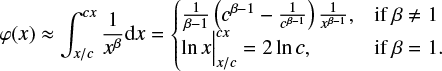
If an empirical probability density function f is close to a power function with an exponent –β, then the corresponding interval probability function (ipf, φ), as an integral of f, is also close to a power function; its exponent being –β + 1:
 (A.1)
(A.1)
We note that this increase of the exponent by one is still valid for the function 1/x, which follows from (A.1) with β − 1 = 0. Using exponential instead of uniform bins in the definition of the ipf reduces the noise at large scales. For example, re-drawing the graphs of Fig. 1 with uniform bins gives inadequate results when A > 103 (we have not illustrated this here).
Appendix B: Maximum likelihood approximations
B.1. Weibull density
The following density
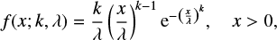 (B.1)
(B.1)
where k > 0 and λ > 0 are shape and scale parameters respectively, determines the Weibull distributions. Given a sample xi, the maximum likelihood method allows one to estimate the parameters k and λ by maximizing the logarithmic likelihood function
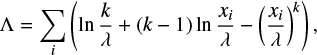 (B.2)
(B.2)
with respect to k and λ. The necessary conditions become, after simplifications,
 (B.3)
(B.3)
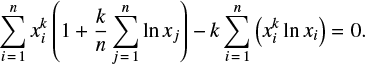 (B.4)
(B.4)
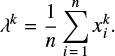
The left hand side of Eq. (B.4) monotonously decreases with respect to k, and we find numerically its solution k. Then λ is computed with Eq. (B.3), Table B.1.
B.2. Truncated power law density
Let [a, b] be the interval of the approximation. Then the truncated power law density is
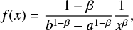 (B.5)
(B.5)
if x ∈ [a,b] and 0 otherwise.  be the sample in question. Maximizing the likelihood function with respect to β, we get the equation
 (B.6)
(B.6)
where the optimal β is the single unknown. Since the left hand side of (B.6) monotonously decreases, we solved the equation numerically. Table 2 reports the values of β computed with this procedure.
Appendix C: Identification procedure
During the course of an Earth day of 24 h, groups rotate with the Sun and increase their longitudes by ld = 360/27.2753. Observations are recorded, in general, at different times of the day so that the longitudes of two consequent records of the same group can differ by more that ld, but this difference is less than 2ld.
Let ltest ∈ [2ld, 180–2ld] be the test longitude. We distributed all observed sizes V into intervals J1 = [1,ν), J2 = [ν, ν2), . . ., whose length grows exponentially; ν is a positive constant chosen to be 1.5. We note as Gr1 the set of groups g such that (i) their records have at least one longitude in the interval [ltest, ltest +2ld]; (ii) the size V(g) of the group g belongs to J1. Among these groups, we select those whose records do not include longitudes l < ltest. In other words, the selected groups are born in [ltest, ltest + 2ld]. Let N+1 be their number, |Gr1| be the number of the groups in Gr1. Then we put ν1 = N+1/|Gr1| and assign this ν1 to the groups such that their records have longitudes in [0, 2l d]; and their sizes V(g) ∈ J1. Passing from J1 to an arbitrary interval Jk, k = 2, 3, . . ., we determine νk in the same manner as ν1 and assign it to the groups such that their records have longitudes in [0, 2ld]; and their sizes V(g) ∈ Jk.
In summary, we find the proportion of groups born in the interval [ltest, ltest + 2ld]. Assuming that this proportion depends only on the length 2ld of the interval, these proportions are taken as the probabilities that a group Jk observed with longitudes in [0,2ld] is a newborn.
Appendix D: Splitting of set G1 into two independent sub-sets
We split the set G1 into two subsets. The division is performed separately for different size ranges. The total range of the group sizes is divided into the intervals J1 = [1, ν), J2 = [ν, ν2), . . ., Jn = [νn−1, νn), where ν = 1.5. Let a group g ∈ G1 have a size V that belongs to some Jk, 1 ≤ k ≤ n. Then this group g is placed in the first subset if the last group g′ found with a size from the interval Jk was placed in the second subset. In other words, let g′ and g be two groups such that (i) their sizes belong to a Jk (ii) no groups recorded between g′ and g have property (i). Then g′ and g are placed into different subsets. In the opposite case the group g is placed in the second subset.
Appendix E: CDF of areas for RGO
 |
Fig. E.1. Complement distribution function Fi(A) = 1 – CDFi(A) = Proba > A of the areas observed on a random day (snapshots), maximal areas of all groups (max1), and of those groups that achieve their maximal areas on longitudes lE ∈ [60, 120] (max2). |
Figure E.1 illustrates the complement cumulative distribution function ℱ(x),
 (E.1)
(E.1)
computed for areas of groups from three subsets. The first subset includes all areas recorded in the catalog (the RGO catalog alone is considered). It gives the snapshot distribution. The second subset contains the maximal areas assigned to each group. The third subset is a part of the second: only the groups whose maximal area is attained at longitudes lE ∈ [60, 120] are considered. The complement distribution function ℱ is computed for each of the subsets (Fig. E.1). Together, the three of them present a power law segment that extends over 0.5 order of magnitude for the snapshot, 1.0 order of magnitude for max1 and somewhat more (1.1) for max2.
References
- Aschwanden, M. 2011, Self-organized Criticality in Astrophysics: the Statistics of Nonlinear Processes in the Universe (Berlin: Springer-Verlag) [CrossRef] [Google Scholar]
- Aschwanden, M., Crosby, N. B., Dimitropoulou, M., et al. 2016, Space Sci. Rev., 198, 47 [NASA ADS] [CrossRef] [Google Scholar]
- Bak, T. J., Tang, C., & Wiesenfeld, K. 1987, Phys. Rev. Lett., 59, 381 [NASA ADS] [CrossRef] [PubMed] [Google Scholar]
- Baumann, I., & Solanki, S. K. 2005, A&A, 443, 1061 [NASA ADS] [CrossRef] [EDP Sciences] [Google Scholar]
- Ben-Hur, A., Biham, O., & Wiesenfeld, K. 1996, Phys. Rev. E, 53, R1317 [NASA ADS] [CrossRef] [Google Scholar]
- Boffetta, G., Carbone, V., Giuliani, P., Veltri, P., & Vulpiani, A. 1999, Phys. Rev. Lett., 83, 4662 [NASA ADS] [CrossRef] [Google Scholar]
- Bogdan, T. J., Gilman, P.-A., Lerche, I., & Howard, R. 1988, ApJ, 327, 451 [NASA ADS] [CrossRef] [Google Scholar]
- Chapman, G. A., Cookson, A. M., & Dobias, J. J. 1997, ApJ, 482, 541 [NASA ADS] [CrossRef] [Google Scholar]
- Chessa, A., Stanley, E. H., Vespignani, A., & Zapperi, S. 1999, Phys. Rev. E, 59, R12 [NASA ADS] [CrossRef] [Google Scholar]
- Crosby, N. B., Aschwanden, M. J., & Dennis, B. R. 1993, Sol. Phys., 143, 275 [NASA ADS] [CrossRef] [Google Scholar]
- Dragulescu, A., & Yakovenko, V. M. 2001, Phys. A, 299, 213 [CrossRef] [Google Scholar]
- Eeckhout, J. 2004, Am. Econ. Rev., 94, 1429 [CrossRef] [Google Scholar]
- Eeckhout, J. 2009, Am. Econ. Rev., 99, 1676 [CrossRef] [Google Scholar]
- Gabaix, X. 1999, Q. J. Econ., 114, 739 [Google Scholar]
- Gutenberg, B., & Richter, R. F. 1944, Bull. Seismol. Soc. Am., 34, 185 [Google Scholar]
- Henwood, R., Chapman, S. C., & Willis, D. M. 2010, Sol. Phys., 262, 299 [NASA ADS] [CrossRef] [Google Scholar]
- Jiang, J., Cameron, R. H., Schmitt, D., & Schüssler, M. 2011, A&A, 528, A82 [NASA ADS] [CrossRef] [EDP Sciences] [Google Scholar]
- Johnson, J. B. 1925, Phys. Rev., 26, 71 [NASA ADS] [CrossRef] [Google Scholar]
- Keilis-Borok, V., Knopoff, L., Rotwain, I., & Allen, C. 1988, Nature, 335, 690 [NASA ADS] [CrossRef] [Google Scholar]
- Kolmogorov, A. N. 1941, in Dokl. Akad. Nauk SSSR, 30, 301 [Google Scholar]
- Kossobokov, V., Le Mouël, J.-L., & Courtillot, V. 2012, Sol. Phys., 276, 383 [NASA ADS] [CrossRef] [Google Scholar]
- Levy, M. 2009, Am. Econ. Rev., 99, 1672 [CrossRef] [Google Scholar]
- Lu, E. T., & Hamilton, R. J. 1991, ApJ, 340, L89 [NASA ADS] [CrossRef] [Google Scholar]
- Lübeck, S., & Usadel, K. D. 1997, Phys. Rev. E, 55, 4095 [NASA ADS] [CrossRef] [Google Scholar]
- Mandelbrot, B. 1960, Int. Econ. Rev., 94, 72 [Google Scholar]
- Manna, S. S. 1991, J. Phys. A, 24, L363 [NASA ADS] [CrossRef] [Google Scholar]
- Mantegna, R. N., & Stanley, H. E. 2000, An Introduction to Econophysics: Correlations and Complexity in Finance (Cambridge, UK: Cambridge University Press) [Google Scholar]
- Marković, D., & Gros, C. 2014, Phys. Rep., 536, 41 [NASA ADS] [CrossRef] [Google Scholar]
- Martinez Pillet, V., Moreno-Insertis, F., & Vazquez, M. 1993, A&A, 274, 521 [NASA ADS] [Google Scholar]
- McIntosh, P. S. 1981, in The Physics of Sunspots, eds. L. Cram, & J. H. Thomas (New Mexico: Sacramento Peak Observatory, Sunspot) [Google Scholar]
- Meunier, N. 2003, A&A, 405, 1107 [NASA ADS] [CrossRef] [EDP Sciences] [Google Scholar]
- Muñoz-Jaramillo, A., Senkpeil, R. R., Windmueller, J. C., et al. 2015, ApJ, 800, 48 [Google Scholar]
- Narkunskaya, G., & Shnirman, M. 1990, Phys. Earth and Planet. Inter., 61, 29 [NASA ADS] [CrossRef] [Google Scholar]
- Parnell, C. 2002, MNRAS, 335, 389 [NASA ADS] [CrossRef] [Google Scholar]
- Parnell, C. E., De Forest, C. E., Hagenaar, H. J., & Johnston, B. A. 2009, ApJ, 698, 75 [NASA ADS] [CrossRef] [Google Scholar]
- Petrovay, K., & Moreno-Insertis, F. 1997, ApJ, 485, 398 [NASA ADS] [CrossRef] [Google Scholar]
- Petrovay, K., & van Driel-Gesztelyi, L. 1997, Sol. Phys., 176, 249 [NASA ADS] [CrossRef] [Google Scholar]
- Rieutord, M., & Rincon, F. 2010, Liv. Rev. Sol. Phys., 7, 1 [NASA ADS] [Google Scholar]
- Roberts, D. C., & Turcotte, D. L. 1998, Fractals, 6, 351 [CrossRef] [Google Scholar]
- Royal Greenwich Observatory 1980, Royal Observatory Annals (Herstmonceux: Royal Greenwich Observatory) [Google Scholar]
- Schad, T. A., & Penn, M. J. 2010, Sol. Phys., 262, 19 [NASA ADS] [CrossRef] [Google Scholar]
- Schrijver, C. J., Title, A. M., van Ballegooijen, A. A., Hagenaar, H. J., & Shine, R. A. 1997, ApJ, 487, 424 [NASA ADS] [CrossRef] [Google Scholar]
- Shapoval, A. B., & Shnirman, M. G. 2005, Int. J. Mod. Phys. C, 16, 1893 [NASA ADS] [CrossRef] [Google Scholar]
- Shapoval, A. B., & Shnirman, M. G. 2012, Phys. A: Stat. Mech. Appl., 391, 15 [CrossRef] [Google Scholar]
- Song, W. G., Zhang, H. P., Chen, R., & Fan, W. C. 2002, Fire Saf. J., 38, 453 [CrossRef] [Google Scholar]
- Stark, C. P., & Hovius, N. 2001, Geophys. Res. Lett., 28, 1091 [NASA ADS] [CrossRef] [Google Scholar]
- Svalgaard, L., & Schatten, K. H. 2016, Sol. Phys., 291, 2653 [Google Scholar]
- Tlatov, A. G., & Pevtsov, A. A. 2014, Sol. Phys., 289, 1143 [Google Scholar]
- Tlatov, A. G., Makarova, V. V., Skorbezh, N. N., & Muñoz-Jaramillo, A. 2016, Kislovodsk Mountain Astronomical Station (KMAS) [Google Scholar]
- Uritsky, V. M., & Pudovkin, M. I. 1998, Ann. Geophys., 16, 1580 [Google Scholar]
- Usoskin, I. G., Kovaltsov, G. A., Lockwood, M., et al. 2016, Sol. Phys., 291, 2685 [Google Scholar]
- Willis, D. M., Wild, M. N., & Warburton, J. S. 2016, Sol. Phys., 291, 2519 [NASA ADS] [CrossRef] [Google Scholar]
- Zhang, J., Wang, Y., Liu, Y., & Hansen, W. W. 2010, ApJ, 723, 1006 [NASA ADS] [CrossRef] [Google Scholar]
- Zharkov, S., Zharkova, V. V., & Ipson, S. S. 2005, Sol. Phys., 228, 377 [NASA ADS] [CrossRef] [Google Scholar]
All Tables
All Figures
|
Fig. 1. Left panel: interval probability function, ipf, φ(A) = ProbA/c ≤ area < Ac, c2 = 1.5, found with the RGO database for all groups observed on any day (snapshot distribution), for maximal observed areas of all groups (max1), and for those whose maximal area is observed at longitudes lE ∈ [60,120] in coordinates associated with Earth observers (max2). Right panel: enlargement of the rectangular window in left part of the figure ( μH are millionths of a solar hemisphere). |
| In the text | |
|
Fig. 2. ipf φ0(V) = Prob{V/c ≤ size < Vc} of the group sizes for the sets G0 of catalogs RGO (28 points in the graph), SOON (26 points), PCSA (28 points), and KMAS (27 points); c2 = 1.5; V is measured in μH. |
| In the text | |
|
Fig. 3. Segments of the size-frequency relations for catalogs RGO, SOON, PCSA, KMAS: ipf φ0 (constructed with set G0), φ1, φ2 (constructed with G1), and φ3 (constructed with G3); c2 = 1.5; vertical (black and blue) lines indicate the 0.95-confidence intervals computed for φ1 and φ3 at point V ≈ 500. V is measured in μH. |
| In the text | |
|
Fig. 4. Segments of the size-frequency relations for catalogs RGO, SOON, PCSA, KMAS: ipf φ1 (circles) are shown together with theoretical values calculated for the power law distribution on the interval [a,b], where [a,b] is [10, 1000], [100, 1000], [10, 1000], [10, 1000] for RGO, SOON, PCSA, and KMAS respectively and with 0.95-confidence intervals illustrated by vertical lines; c2 = 1.5. V is measured in μH. |
| In the text | |
|
Fig. 5. χ2-probability (panel a) and the exponent (panel b) of the power law distribution versus the left boundary of the power law interval; 2000 is assigned to the right boundary; the logarithmic length of the bins is c = 1.2; The smallest values of the PCSA curve are 0.006 and 0.002. |
| In the text | |
|
Fig. 6. Verification procedures applied successively: sorting of the outgoing groups, identification and elimination of incoming groups, and subdivision of the sets G1 and G3 into subsets to check the stability of the observed power law segments (see text). |
| In the text | |
|
Fig. 7. ipf of sizes (φ3, ×-marked graph) and corrected sizes obtained by linear extrapolation and interpolation with respect to areas (φr,a, plus-marked graph), and with respect to the square root of area respectively (φr,l, circle-marked graph). Best fits with Weibull distributions computed on the intervals [10, +∞), [100, +∞), and [10,1000) are given as ipf with solid, dashed, and dash-dotted lines respectively; c2 = 1.5. V is measured in μH. |
| In the text | |
|
Fig. 8. ipf of sizes (φ3, ×-marked graph) and corrected sizes obtained by linear extrapolations with respect to the square root of areas (φ3,l, circle-marked graph); c2 = 1.1. |
| In the text | |
|
Fig. E.1. Complement distribution function Fi(A) = 1 – CDFi(A) = Proba > A of the areas observed on a random day (snapshots), maximal areas of all groups (max1), and of those groups that achieve their maximal areas on longitudes lE ∈ [60, 120] (max2). |
| In the text | |
Current usage metrics show cumulative count of Article Views (full-text article views including HTML views, PDF and ePub downloads, according to the available data) and Abstracts Views on Vision4Press platform.
Data correspond to usage on the plateform after 2015. The current usage metrics is available 48-96 hours after online publication and is updated daily on week days.
Initial download of the metrics may take a while.